On stable controller design for robust stabilization of time delay systems

(1)

ScienceDirect

IFAC-PapersOnLine 48-12 (2015) 404–409

Available online at www.sciencedirect.com

On Stable Controller Design For Robust

Stabilization of Time Delay Systems

Veysel Y¨ucesoy∗ _{Hitay ¨}_Ozbay∗∗

∗

Bilkent University 06800 Bilkent, Ankara, Turkey (e-mail: vyucesoy@ee.bilkent.edu.tr).

∗∗

Bilkent University 06800 Bilkent, Ankara, Turkey (e-mail: hitay@bilkent.edu.tr)

Abstract: This paper studies the problem of robust stabilization of an infinite dimensional plant by a stable and possibly low order controller. The plant of interest is assumed to have only finitely many simple unstable zeros, however, may have infinitely many unstable poles. In the literature, it has been shown that the problem can be reduced to an interpolation problem and it is possible to obtain lower and upper bounds of the multiplicative uncertainty under which an infinite dimensional stable controller can be generated by a modified Nevanlinna-Pick formulation. We propose that the same interpolation problem can be solved approximately by a finite dimensional approach and present a finite dimensional interpolation function which can be used to find a stable controller. We illustrate this idea by a numerical example and additionally show the effects of the free design parameters of the rational interpolating outer function approach on the numerical example.

Keywords: Strong stabilization, robust stabilization, infinite dimensional systems, H∞

control, low degree controller

1. INTRODUCTION

This paper is about strong and robust stabilization of SISO infinite dimensional plants, specifically time delay systems, by a finite dimensional controller. Strong stability requires a stable controller to be designed. A stable controller has two main advantages: it is robust to sensor failures (i.e. undetermined feedback input or saturation of control input) as described by Doyle et al. (1990), and ¨Unal and ˙Iftar (2012c) and it is testable stand-alone as mentioned by van de Wal et al. (2002). It is possible to test a stable controller by its input-output relationship practically by applying some test signals as an open-loop system before using it with the original plant to prevent undesired errors. It is essential to mention that strong stability means achieving stabilization by a stable controller which is different than some other strong stability concepts used in the infinite dimensional system theory, e.g. Hale and Lunel (2002).

There is a rich literature for strong stabilization of fi-nite dimensional plants, see e.g. Campos-Delgado and Zhou (2003), Cheng et al. (2007), Cheng et al. (2011), Gümü¸ssoy and Özbay (2009), Petersen (2009), and Günde¸s and Özbay (2011) and see also Gümü¸ssoy et al. (2008) for sensitivity shaping of infinite dimensional systems by fixed order stable controllers. Nevertheless, robust stabilization by a stable controller remains to be an active open research area and to our knowledge; the most recent contribution, which has been made by Wakaiki et al. (2013), gives some sufficient conditions as discussed below in more de-tail. Most recently, the same idea has been extended to

the mixed sensitivity minimization by stable controllers, Wakaiki and Yamamoto (2014); see also G¨um¨u¸ssoy and

¨

Ozbay (2009) for an alternative earlier approach. We refer to ¨Unal and ˙Iftar (2012b) and ¨Unal and ˙Iftar (2012c) for recent results on stable H∞

controller design for plants with input-output delays. It should be noted that for time delay systems, parity interlacing property, p.i.p., (having even number of poles between any pair of extended right half plane zeros) is necessary (and sufficient with added restrictions) for the existence of a strongly stabilizing controller, ¨Unal and ˙Iftar (2012a).

In their paper, Wakaiki et al. (2013) have studied infinite dimensional plants having finitely many simple unstable zeros but possibly infinitely many unstable poles. The au-thors have tried to find a way to calculate upper and lower bounds for the largest multiplicative uncertainty under which a robustly stabilizing stable controller can be gen-erated. They have used a method developed in Gümü¸ssoy and Özbay (2009) and Özbay (2010), where an extension to the well known Nevanlinna-Pick interpolation algorithm is used. After calculating the upper and lower bounds, Wakaiki et al. (2013) also proposed how to generate a stable controller for a given multiplicative uncertainty. In this approach, for each bound, a modified version of the Nevanlinna-Pick interpolation problem is solved and the resulting interpolating function is an infinite dimensional one. Since this interpolating function is a part of the designed controller, the resulting controller ends up to be infinite dimensional, independent of the other components. In this paper, we present an application of an old method appearing in Vidyasagar (1985) and Doyle et al. (1990),

Proceedings of the 12th IFAC Workshop on Time Delay Systems June 28-30, 2015. Ann Arbor, MI, USA

On Stable Controller Design For Robust

Stabilization of Time Delay Systems

Veysel Y¨ucesoy∗ _{Hitay ¨}_Ozbay∗∗

∗

∗∗

1. INTRODUCTION

¨

On Stable Controller Design For Robust

Stabilization of Time Delay Systems

Veysel Y¨ucesoy∗

Hitay ¨Ozbay∗∗

∗

∗∗

1. INTRODUCTION

¨

On Stable Controller Design For Robust

Stabilization of Time Delay Systems

Veysel Y¨ucesoy∗

Hitay ¨Ozbay∗∗

∗

∗∗

1. INTRODUCTION

¨

(2)

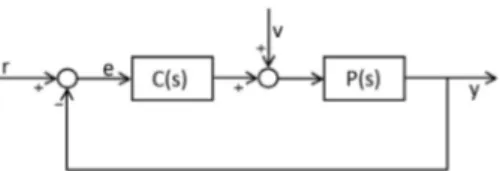
Fig. 1. The standard unity feedback system.

where a finite dimensional approach is used to find an interpolating outer function, without considering the H∞

norm condition to be satisfied for robustness. We apply this method to solve the relaxed problems described by Wakaiki et al. (2013) to calculate “approximate” upper and lower bounds, then check the resulting H∞

norm condition to verify that the stable controller designed also satisfies the robustness condition.

The paper is organized as follows: in Section 2 some details and brief results from Wakaiki et al. (2013) are presented. In Section 3 the method proposed in Vidyasagar (1985) and Doyle et al. (1990) is recalled and it is applied to the relaxed problems to calculate approximate maximum allowable uncertainty bounds. The effects of different free design parameters on the numerically calculated interpo-lation function are investigated in Section 5. Finally, Sec-tion 6 contains some concluding remarks on the proposed method.

2. PROBLEM DEFINITION

In this paper, we consider the feedback system shown in Figure 1 where C is required to be a stable controller, i.e. C ∈ H∞

, for a given infinite dimensional plant P . Recall that the feedback system (C, P ) is stable if and only if S = (1 + P C)−1

, CS and P S are H∞

functions. A controller C ∈ H∞

leading to a stable feedback system (C, P ), is said to be a strongly stabilizing controller for the given plant P .

In this paper we consider the same class of plants consid-ered in Wakaiki et al. (2013):

P = N

D (1)

such that N ∈ H∞

, D ∈ H∞

and the pair (N, D) are strongly co-prime as in Smith (1989). A controller strongly stabilizing P is a robustly stabilizing controller for the set

Pρ := {P∆= (1 + W ∆)P :

∆ ∈ H∞

, �∆�∞< 1/ρ}

(2) if and only if it satisfies

�W T �∞≤ ρ (3)

where T = P C(1 + P C)−1

, and W characterizes the fre-quency distribution of the multiplicative plant uncertainty. In this work we assume that W, W−1

∈ H∞

.

As in Wakaiki et al. (2013) we consider an inner-outer factorization of N and D so that

P = Mn Md

N0 (4)

where Mn is inner and finite dimensional, Mdis inner and

possibly infinite dimensional and N0, N −1 0 ∈ H

∞

.

Note that when Md is infinite dimensional the plant

contains infinitely many poles in C+ (e.g. a neutral time

delay system with asymptotic pole chains in C+); however

requiring N−1

0 ∈ H∞ imposes a restriction that the plant

is not strictly proper.

Example: A typical plant example satisfying the above conditions is the neutral time delay system

P (s) = (s − α)(s − 4e

−s_{+ 1)}

(s − 10)(s − 15)(2e−s_{+ 1)} (5)

where the factorization is in the form Mn(s) := (s − α)(s − p) (s + α)(s + p) Md(s) := (s − 10)(s − 15)(2e−s+ 1) (s + 10)(s + 15)(e−s_{+ 2)} No(s) := (s + α)(s + p)(s − 4e−s_{+ 1)} (s − p)(s + 10)(s + 15)(e−s+ 2) (6)

with p > 0 being the only root of the quasi-polynomial (s − 4e−s_{+ 1) in C}

+; p can be calculated numerically

by using qpmr or Yalta packages, see Vyhl´ıdal and Z´ıtek (2014) and Avanessoff et al. (2013); for the above example, p = 0.7990.

In the rest of the paper, it is assumed that W = KW0

where both W0and W0−1belong to H∞and K > 0. Thus

we have robust stability if �W0T �∞<

1

ρ K. (7)

Problem Definition: In summary, the problem at hand is to find a strongly stabilizing C for P satisfying (7) for the largest possible K. We call the largest K > 0 for which the above problem is solvable the largest allowable

uncertainty bound. By ¨Unal and ˙Iftar (2012a), in order to

have a feasible solution to the strong stabilization problem, P is assumed to satisfy the parity interlacing property. In Wakaiki et al. (2013) some upper and lower bounds are computed for the largest allowable uncertainty bound. Brief Outline of the Proposed Solution: Wakaiki et al. (2013) showed that for a given K > 0 the strong robust stabilization problem is solvable if and only if there exists a function F satisfying all three conditions given below: F, F−1 ∈ H∞ (8) �W − MdF �∞≤ ρ (9) F (zi) = W (zi) Md(zi) , i = 1, ..., n, (10) where z1, . . . , zn are the zeros of P in C+. Furthermore,

once such a function F is constructed, a feasible controller is given by

C = W − MdF

MnN0F (11)

Since the above problem is not straight forward to solve, Wakaiki et al. (2013) have proposed two relaxed problems each of which defines a necessary (respectively, a suffi-cient) condition to calculate upper and lower bounds for the largest possible multiplicative uncertainty K. In the relaxed problem, which is designed to solve for the lower bound, they have defined Wsto be Ws, Ws−1∈ RH

∞

such that |Ws(jω)| ≤ ρ−|W (jω)| for almost all ω ∈ R. If finitely

(3)

then we define βi= W (zi)/(Md(zi)Ws(zi)) for i = 1, ..., n.

Wakaiki et al. (2013) proved that if G is a solution to the modified Nevanlinna-Pick problem with the interpolation data (zi, βi)ni=1 then

C = W − MdWsG MnN0WsG

(12) is a solution for the strong and robust stabilization problem. A similar definition is given by Wakaiki et al. (2013) for the upper bound calculations and it relies on a solution of another modified Nevanlinna-Pick problem.

Modified Version of Nevanlinna-Pick Problem: Suppose z1, ..., zn ∈ C+ are distinct and none of them

coincide with s = 1; let β1, ..., βn ∈ C \ {0}. Determine

whether there exists a function G such that G, G−1

∈ H∞

, �G�∞≤ 1 and G(zi) = βi for i = 1, ..., n.

The condition G−1

∈ H∞

is the modification on the original Nevanlinna-Pick problem. The modified version of the problem is proved to be solvable by Gümü¸ssoy and Özbay (2009) and Özbay (2010) if and only if there exists an integer set [k1, ..., kn] such that Pick matrix

P([k1, ..., kn]), P([k1, ..., kn]) := − log βp− log βq+ j2π(kq− kp) 1 − φ(zp)φ(zq) n p,q=1 (13) is positive semi definite where

φ : C+→ D : φ(s) =

s − 1

s + 1. (14)

Wakaiki et al. (2013) have given a solution to the modified Nevanlinna-Pick problem which ends up with an infinite dimensional G appearing in the designed controller, (12). As a result, the generated controller solves the strong

and robust stabilization problem for an infinite dimensional

plant with an infinite dimensional controller.

Remark. By the above design in (12), F = WsG

is outer. In order to guarantee a bound on �F−1

�∞,

Gümü¸ssoy and Özbay (2009) proposes a modified version of the Nevanlinna-Pick interpolation, where a parameter σ appears, so that �F−1

�∞≤ e

σ_{. In the numerical example}

considered below, we will use a relatively large σ and illustrate that this leads to a large controller gain at low frequencies.

3. AN INTERPOLATING RATIONAL OUTER FUNCTION

In Vidyasagar (1985) (see also Doyle et al. (1990)) a constructive method is outlined to generate a rational interpolating function, say U , which is guaranteed to be outer (i.e. both the function itself and its inverse are stable)1 _{under some constraints related to parity}

interlacing property.

Let us assume that we have some ai ∈ C+ and bi as the

interpolation data in the way U (ai) = bi for i = 1, ..., n.

1 _{An outer function need not be invertible in H}∞

, in fact we seek

an outer function whose inverse is also in H∞

, such functions are

called unimodular in H∞

. But we will look for an outer function, then using a parameter σ > 0 as in the above remark, we will put a bound on the inverse of the interpolating outer function, using an

idea from Gümü¸ssoy and Özbay (2009).

Define U1(s) = b1, so that U1(a1) = b1, clearly U1is outer

and satisfies the first interpolation condition. Now suppose that an outer Uk is constructed in such a way that it

satisfies the first k interpolation conditions for 1 ≤ k < n. Then, it is possible to define Uk+1 as

Uk+1(s) = (1 + ck+1Hk+1(s))lUk(s) (15)

where Hk+1 ∈ H∞ and such that Hk+1(ai) = 0 for

i = 1, ..., k. This choice of Hk+1 makes Uk+1(ai) = Uk(ai)

for i = 1, ..., k independent of c and l. As a result, Uk+1 is

guaranteed to satisfy the interpolation data (ai, bi)ki=1. If

it is possible to choose c and l such that Uk+1(ak+1) =

bk+1 and |ck+1| < 1/�Hk+1�∞ then Uk+1 satisfies the

interpolation data (ai, bi)k+1i=1 and it is outer. At the end of

the algorithm, U = Un satisfies all the interpolation data

and is outer.

By this method, it is possible to generate interpolating ra-tional outer functions. It is also possible to tune the degree of the outer function by changing the value of parameter l, when c does not satisfy the norm condition. One additional important point is the choice of Hi functions. Due to

the imposed requirements, zero location of the function is obvious (i.e. zeros of Hkhave to be at aifor i = 1, ..., k−1).

However, the pole location is not constrained by the re-quirements. This means that the pole location can be a free design parameter to be determined to shape the resulting interpolation function. If we recall the requirements of the modified Nevanlinna-Pick problem from Section 2, we seek for an outer function G satisfying certain interpolation data, and a norm condition as �G�∞ < 1. The method

described in this section gives a function satisfying the first two conditions (i.e. interpolation data and being outer) but not necessarily the norm constraint.

4. A COMPUTATIONAL METHOD FOR THE PROBLEM SOLUTION

In this section, we try to make use of the method in Section 3 in order to find a norm constrained interpolating rational outer function to solve the modified Nevanlinna-Pick problem defined in Wakaiki et al. (2013).

Let us first recall the problem definition. The problem data: zi for i = 1, ..., n are the unstable zeros of the plant

P (they are assumed to be distinct). The problem is to find a G such that

G(zi) = βi G ∈ H∞ G−1 ∈ H∞ �G�∞< 1. Proposed Algorithm:

• Define r = (r1, ..., rn) to be the relative pole location

for the corresponding zi within each Hk which will

be a part of the interpolation operation. (i.e. r = (1, ..., 1) is the case called as fixed pole location) • Use the inner-outer factorization of the plant as given

in (6), P = MdN0/Mn

• Define lmax to be the maximum allowable relative

degree for the interpolant G.

• At each step fix r to find maximum possible K as follows:

(4)

- Define W = KW0 with current K

- Estimate Ws by using the MATLAB function

fitmagfrdas explained in Wakaiki et al. (2013) - Calculate βi = W (zi)/Md(zi)Ws(zi) for i = 1, ...n - Let U1(s) = β1 fork = 2 : n while(l < lmax) Uk = (1 + ckHk)lUk−1 Find ck from Uk(zk) = βk if ((�Uk�∞< 1) and (ck < 1/�Hk�∞))

Conditions are satisfied, break while else l = l + 1 end if end while end for G = Un if a feasible G is constructed increase K else decrease K end if end while

The proposed algorithm is best explained with an example. 5. AN ILLUSTRATIVE EXAMPLE

Wakaiki et al. (2013) have studied a numerical example and derived upper and lower bounds for the multiplicative uncertainty under which a stable controller can be gener-ated. The example is formed by the plant given in (5) and the factorization in (6) and the rest of the problem data is as follows: W (s) = K s + 1 s + 10 ρ = 1 2 ≤ α < 10 K > 0                  (16)

See Figure 2 of Wakaiki et al. (2013) for the lower and upper bounds of the largest allowable K for which the robust strong stabilization problem is solvable with data given in (16) for the plant (5), with α ∈ (2 , 10). In what follows we illustrate the application of the algorithm proposed in Section 4. Our objective is to find a finite dimensional G as an alternative to the infinite dimensional one constructed in Wakaiki et al. (2013).

5.1 Interpolating Rational Outer Function by an Inner

H(s)

Having reached the original results from Wakaiki et al. (2013), we started to replace the interpolation function generating part with the method of Section 3. For the given numerical example, Wsand Wnare generated by Matlab

built-in function fitmagfrd and the interpolation data calculated as z1 = α, β1 = W (α)/(Md(α)Ws(α)) and

z2= p = 0.7990, β2= W (p)/(Md(p)Ws(p)). Recall that p

is the only unstable zero of the infinite dimensional part of the plant and α is the simple zero of the plant. The

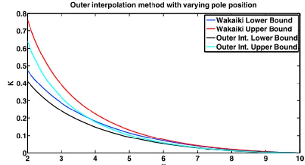
2 3 4 5 6 7 8 9 10 0 0.1 0.2 0.3 0.4 0.5 0.6 0.7 0.8 α K

Outer interpolation method with varying pole position Wakaiki Lower Bound Wakaiki Upper Bound Outer Int. Lower Bound Outer Int. Upper Bound

Fig. 2. Upper and lower bounds calculated for the maxi-mum allowable multiplicative uncertainty by a finite dimensional interpolation function which is generated by the outer interpolation method of Section 3 using varying pole location in H(s) as the interstage func-tion, having degree l < 5.

2 3 4 5 6 7 8 9 10 0 0.1 0.2 0.3 0.4 0.5 0.6 0.7 0.8 α K

Outer interpolation method with varying pole position + varying degree Wakaiki Lower Bound Wakaiki Upper Bound Outer Int. Lower L = 3 Outer Int. Lower L = 5 Outer Int. Lower L = 7 Outer Int. Lower L = 10

Fig. 3. Lower bounds calculated for the maximum allow-able multiplicative uncertainty by a finite dimensional interpolation function which is generated by the outer interpolation method of Section 3 using varying pole location in H(s) as the interstage function, having degree l ∈ {3, 5, 7, 10}.

objective is to calculate the maximum allowable multi-plicative uncertainty bound under which a stable robust controller can be generated. Ws is replaced by Wn for

upper bound calculations. Since we have two interpolation conditions, and both zeros are real, we just need to design a single H function for the second interpolation phase. The simplest and immediate choice is H(s) = (s−α)_(s+α) for which H becomes inner. It is observed that the bounds calculated by this choice of H are far away from the bounds determined in Wakaiki et al. (2013). So, the next step is to investigate different choices of H and if necessary increase the order l.

5.2 Outer Interpolation by Varying Pole Location

After having the unsatisfactory results which are explained in Section 5.1, we now introduce a new parameter to the problem as the pole location of the interstage function H. Accordingly, set H(s) = _(s+rα)(s−α) where r > 0 is the design parameter. We search for the optimum r which maximizes the upper and lower bounds for a fixed α. The results are shown in the Figure 2.

As it was clearly observed that letting pole location to vary, instead of fixing it to make H inner, significantly improves both the upper and lower bound approximations. It is also important to understand what upper and lower

(5)

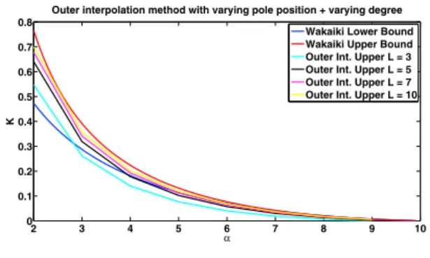
2 3 4 5 6 7 8 9 10 0 0.1 0.2 0.3 0.4 0.5 0.6 0.7 0.8 α K

Outer interpolation method with varying pole position + varying degree Wakaiki Lower Bound Wakaiki Upper Bound Outer Int. Upper L = 3 Outer Int. Upper L = 5 Outer Int. Upper L = 7 Outer Int. Upper L = 10

Fig. 4. Upper bounds calculated for the maximum allow-able multiplicative uncertainty by a finite dimensional interpolation function which is generated by the outer interpolation method of Section 3 using varying pole location F (s) as the interstage function, having degree l ∈ {3, 5, 7, 10}.

bounds mean in terms of the solution of the modified Nevanlinna-Pick problem. In the formulation derived by Wakaiki et al. (2013), lower bound is the bound under which the defined problem is certainly solvable by the given solution method (i.e. by calculating an infinite di-mensional G). Similarly, upper bound is the bound above which the defined problem is certainly not solvable by the given solution method. In other words, for a fixed α in Figure 2 of Wakaiki et al. (2013), the optimum multi-plicative uncertainty K under which a stable but infinite dimensional controller can be generated is between the defined upper and lower bounds. When this explanation is considered, the expected behavior of the approximated up-per and lower bounds is to approach from above and from below, respectively. Figure 2 suggests that approximate lower bound behaves as expected whereas the approximate upper bound also approaches from below. To be sure about the approaching direction of the bounds an extra computa-tion is done. In this computacomputa-tion, the varying pole locacomputa-tion technique described in this section is used for some differ-ent values of l ∈ {3, 5, 7, 10} to visualize the approaching direction of the approximate bounds calculated by the technique of Section 3. Figure 3 clearly shows that the approximate lower bound approaches from below to the original lower bound calculated by Wakaiki et al. (2013) as expected. However, as Figure 4 depicts the approximate upper bound also approaches to the original upper bound calculated by Wakaiki et al. (2013) from below. This unex-pected behavior seems to grant a better upper bound than the original bound as a first impression, however, since the problems which are solved to generate the bounds are relaxed versions of the original problem, an approximate solution for the upper bound calculation is not meaningful. On the contrary, any approximate solution for the lower bound which stays strictly below the original bound is a suboptimal solution to the original problem. We make use of this fact to generate a low order interpolation function G for the case when α = 2, l = 5, K = 0.4117, r = 0.2046 as given in (17) and the controller is given by (18). The comparison of the controller and G function designed by Wakaiki et al. (2013) and designed by the newly proposed method are given in Figures 5, 6, and 7. The resulting finite dimensional G is outer, i.e. both G, G−1

∈ H∞

. The inter-polation data that is required for the given value of K = 0.4117 is calculated by β1,2 = W (z1,2)/Md(z1,2)Ws(z1,2) 10−5 10−4 10−3 10−2 10−1 100 101 102 103 −300 −250 −200 −150 −100 −50 0 50 ω Magnitude (dB) |G(jω)| Proposed Method Wakaiki’s Method

Fig. 5. The magnitude plots of G(jω) obtained by Wakaiki et al. (2013) and by the proposed algorithm, using l = 5, when α = 2. 10−5 ₁₀−4 ₁₀−3 ₁₀−2 ₁₀−1 ₁₀0 ₁₀1 ₁₀2 ₁₀3 −50 0 50 100 150 200 250 300 ω Magnitude (dB) |C(jω)| Proposed Method Wakaiki’s Method

Fig. 6. The magnitude plot of the calculated C(s) functions by both methods with α = 2, and l = 5 for the proposed method. 100 ₁₀1 ₁₀2 ₁₀3 −10 0 10 20 30 40 ω Magnitude (dB) |C(jω)| Proposed Method Wakaiki’s Method

Fig. 7. Magnitude plot of the controller in the high frequency region.

for z1 = α = 2 and z2 = p = 0.7990 that turn out to be

(zi, βi) = {(0.7990, 0.1275), (2, 0.3955)}. For the constraint

�G−1

�∞≤ e

σ_{, we take σ = 30. It is a simple exercise to}

check that G(0.7990) = 0.1275 and G(2) = 0.3955 by using (17). As the last remark, Figure 5 shows that �G�∞≤ 1;

moreover �G−1

�∞ ≤ 5.7 × 10

12 _{< 1.0686 × 10}13 _{= e}30_.

Thus, the function G constructed here is an admissible solution to the modified Nevanlinna-Pick problem.

G(s) = (s + 0.001147) 5 (s + 0.4091)5 (17) C = W − MdWsG MnN0WsG (18) Note that robust stabilization problem requires N−1

0 to be

a factor of the controller which means exact cancelation of the minimum phase part of the plant. However, robust stabilization problem considered here deals with uncertain

(6)

plants of the form (2), characterized by the weight W . If it is dangerous to invert some portions of N0 then,

the uncertainty weight W must be chosen accordingly. In particular, as in (5) if there are infinitely many poles in C₊_{, any parametric uncertainty in the time delay in M}_d_of (6) puts the problem outside the framework of uncertainty description of (2).

6. CONCLUSIONS

We have obtained some preliminary results towards robust stabilization of an infinite dimensional system with a possibly low order and stable controller. The plant of interest can only have finitely many unstable zeros but may posses infinitely many unstable poles. The strong and robust stabilization of such a plant was studied by Wakaiki et al. (2013) where the authors have proposed two relaxed problems to calculate lower and upper bounds for the multiplicative uncertainty under which a stable but infinite dimensional controller can be generated.

This paper is a first step to solve these relaxed problems by a finite dimensional controller using the rational in-terpolating outer function method of Section 3: the inter-polant G is finite dimensional. We used the same numerical example as Wakaiki et al. (2013) and developed a finite dimensional outer G to achieve robust stabilization. We examined the effects of pole location of the interpolating function and relative degree of G on lower and upper bounds and concluded that the approximations get bet-ter as the degree increases for the lower bound. We also explained why it is not a good idea to solve the relaxed problem for the upper bound by an approximate approach. In future studies we will extend this method to obtain finite dimensional strongly and robustly stabilizing con-trollers by using approximations of Md and N0 together

with the finite dimensional G obtained here. Extension of the method to MIMO plants is also an interesting open problem.

REFERENCES

Avanessoff, D., Fioravanti, A., and Bonnet, C. (2013). Yalta: A matlab toolbox for the hinfty-stability analysis of classical and fractional systems with commensurate delays. 5th IFAC SSSC Grenoble, pp. 839–844.

Bonnet, C., Fioravanti, A., and Partington, J. (2011). Stability of neutral systems with commensurate delays and poles asymptotic to the imaginary axis. SIAM J.

Control Optim, vol. 49, pp. 498–516.

Cheng, P., Cao, Y.Y., and Sun, Y. (2007). On strong γk − γcl H∞ stabilization and simultaneous γk − γcl

H∞

control. Proc. 46th IEEE Conf. Decision Control

(CDC2007), New Orleans, LA, pp. 5417–5422.

Cheng, P., Cao, Y.Y., and Sun, Y. (2011). A new LMI method for strong γk − γcl H∞ stabilization.

Proc. 9th IEEE Intl. Conf. on Control and Automation (ICCA2011), Santiago, Chile, pp. 94–99.

Doyle, J.C., Francis, B.A., and Tannenbaum, A. (1990).

Feedback Control Theory. Macmillan, New York.

Campos-Delgado, D.U., and Zhou, K. (2003). A para-metric optimization approach to H∞ and H2 strong

stabilization. Automatica, 39, 1205–1211.

G¨um¨u¸ssoy, S., Millstone, M., and Overton, M.L. (2008). H∞

strong stabilization via HIFOO, a package for fixed-order controller design flow controller design using approximation of FIR filters. Proc. 47th IEEE CDC, Cancun, pp. 4135–4140

Gümü¸ssoy, S., and Özbay, H. (2008). Stable H∞

controller design for time-delay systems. International Journal of

Control, vol. 81, pp. 546–556.

Gümü¸ssoy, S. and Özbay, H. (2009). Sensitivity mini-mization by strongly stabilizing controllers for a class of unstable time-delay systems. IEEE Transaction on

Automatic Control, vol. 54, pp. 590–595.

G¨unde¸s, A. and ¨Ozbay, H. (2011). Strong stabilization of a class of MIMO systems. IEEE Transaction on Automatic Control, vol. 56, pp. 1445–1451.

Hale, J.K. and Lunel, S.M.V. (2002). Strong stabilization of neutral functional differential equations. IMA Journal

of Mathematical Control and Information, vol. 19, pp. 5–

23. ¨

Ozbay, H. (2010). Stable H∞

controller design for systems with time delays. Perspectives in Mathematical

Sys-tem Theory, Control, and Signal Processing, Springer-Verlag, pp. 105–113.

Petersen, I.R. (2009). Robust H∞

control of an uncertain system via a stable output feedback controller. IEEE

Trans. Automat. Control, vol. 54, pp. 1418–1423.

Smith, M. (1989). On stabilization and the existence of co-prime factorizations. IEEE Transactions on Automatic

Control, vol. 34, pp. 1005–1007.

¨

Unal, H.U. and ˙Iftar, A. (2012a). Strong Stabilization of Time-Delay System. Preprints of the 10th IFAC Workshop on Time Delay Systems (TDS 2012), Boston,

MA, pp. 272–277. ¨

Unal, H.U. and ˙Iftar, A. (2012b). Stable H∞

controller design for systems with multiple input/output time-delays Automatica, vol. 48, pp. 563–568.

¨

Unal, H.U. and ˙Iftar, A. (2012c). Stable H∞

flow controller design using approximation of FIR filters. Trans. Inst.

Meas. Control, vol. 34, pp. 3–25.

van de Wal, M., van Baars, G., Sperling, F., and O.Bosgra (2002). Multivariable H∞

/µ feedback control design for high-precision wafer stage motion. Control Eng. Pract., vol. 10, 739–755.

Vidyasagar M (1985). Control System Synthesis: A

Fac-torization Approach, MIT Press, Cambridge MA.

Vyhl´ıdal, T. and Z´ıtek, P. (2014). Qpmr-quasi-polynomial root-finder: Algorithm update and examples. In Delay

Systems, 299–312. Springer.

Wakaiki, M., and Yamamoto, Y. (2014). Stable con-troller design for mixed sensitivity reduction of infinite-dimensional systems. Systems & Control Letters, vol 72, pp. 80–85.

Wakaiki, M., Yamamoto, Y., and ¨Ozbay, H. (2013). Stable controllers for robust stabilization of systems with in-finitely many unstable poles. Systems & Control Letters, vol. 62, pp. 511–516.