Shoe-leather and 'bricks-and-mortar' as inputs into transaction technology

‘SHOE-LEATHER’ AND ‘BRICKS-AND-MORTAR’ AS INPUTS INTO TRANSACTION TECHNOLOGY

A Master’s Thesis by ÜLKEM BAŞDAŞ Department of Economics Bilkent University Ankara August 2007

To Şükrü Başdaş, Meral Başdaş and Özgü Başdaş for their support at every step I take and giving me the joy of being a real family

‘SHOE-LEATHER’ AND ‘BRICKS-AND-MORTAR’ AS INPUTS INTO TRANSACTION TECHNOLOGY

The Institute of Economics and Social Sciences of

Bilkent University

by

ÜLKEM BAŞDAŞ

In Partial Fulfillment of the Requirements for the Degree of MASTERS OF ARTS in THE DEPARTMENT OF ECONOMICS BILKENT UNIVERSITY ANKARA August 2007

I certify that I have read this thesis and have found that it is fully adequate, in scope and in quality, as a thesis for the degree of Master of Arts in Economics.

--- Dr. Neil Arnwine Supervisor

I certify that I have read this thesis and have found that it is fully adequate, in scope and in quality, as a thesis for the degree of Master of Arts in Economics.

--- Dr. Kıvılcım Metin Özcan Examining Committee Member

I certify that I have read this thesis and have found that it is fully adequate, in scope and in quality, as a thesis for the degree of Master of Arts in Economics.

--- Prof. Şaziye Gazioğlu

Examining Committee Member

Approval of the Institute of Economics and Social Sciences

--- Prof. Erdal Erel Director

ABSTRACT

‘SHOE-LEATHER’ AND ‘BRICKS-AND-MORTAR’ AS INPUTS INTO TRANSACTION TECHNOLOGY

Başdaş, Ülkem

M.S., Department of Economics Supervisor: Dr. Neil Arnwine

August 2007

This thesis explains the difference between the long run and short run income and interest elasticities of money demand by the presence of a fixed input into the creation of transactions in a cash-in advance model of money demand. This structure implies a time element for the response of money demand to changes in income and interest. The implication of the fixed input into the consumer’s transactions technology causes the income elasticity of money demand to be more elastic in short run whereas the interest rate elasticity to be more elastic in the long run. Besides, the presence of a fixed input provides a micro foundation for price stickiness and a time dynamic welfare cost of inflation. Empirical evidence from the US over 1959:1 – 2006:4 period verifies the predictions of our theoretical model on elasticities. To demonstrate that the theoretical model explains observed price stickiness, we use the empirical model to derive a version of the P-Star model of sticky prices. The estimated parameters point out the higher relative productivity of fixed input than of variable input, and a considerably high welfare cost of inflation.

Keywords: Money Demand, Interest and Income Elasticities of Money Demand, Cash-in-advance model, P-Star Model, Welfare Cost of Inflation

ÖZET

İŞLEM TEKNOLOJİSİNDE GİRDİ OLARAK

‘AYAKKABI ESKİTME’ VE ‘TUĞLA-ÇİMENTO’ MALİYETLERİ Başdaş, Ülkem

Yüksek Lisans, İktisat Bölümü Tez Danışmanı: Dr. Neil Arnwine

Ağustos 2007

Bu tez, para talebinin kısa ve uzun dönemdeki gelir ve faiz esneklikleri arasındaki farkı, ön ödeme kısıtlı para talebi modelinde piyasa işlemlerinde sabit girdi tanımlayarak açıklamaktadır. Bu şekilde tanımlanmış teorik model, para talebinin faiz ve gelir esnekliğinin zaman değişkeni içermesini sağlamaktadır. Tüketicinin işlem teknoloji fonksiyonunda sabit girdi tanımlanmasının neticesinde, paranın gelir esnekliği kısa dönemde daha esnek iken, para talebinin faiz esnekliği uzun dönemde daha esnek olmaktadır. Ayrıca, sabit girdinin kullanılması mikro dayanaklı fiyat yapışkanlığını ve enflasyonun refah maliyetinin dinamik olmasını sağlamaktadır. 1959:1 – 2006:4 dönemi için Amerika Birleşik Devletleri’nden alınan empirik bulgular teorik modelin öngördüğü gelir ve faiz esnekliklerini doğrulamaktadır. Teorik modelin gözlemlenen fiyat yapışkanlığını açıklamak için, Potansiyel Fiyat Modeli türünde fiyat yapışkanlığı ile oluşturulan empirik model kullanılmıştır. Tahmin edilen parametreler sabit girdinin göreceli verimliliğinin değişken girdininkinden fazla olduğuna ve enflasyonun refah maliyetinin oldukça yüksek olduğuna işaret etmektedir.

Anahtar Kelimeler: Para Talebi, Para Talebinin Faiz ve Gelir Esnekliği, Ön Ödeme Kısıtlı Para Talebi Modeli, Potansiyel Fiyat Model, Enflasyonun Refah Maliyeti

ACKNOWLEDGEMENTS

I would like to thank to Dr. Neil Arnwine for his patience, careful supervision and guidance through the development of this thesis.

I am indebted to Dr. Kıvılcım Metin Özcan for her valuable support and comments.

I would like to express my gratitude to Prof. Şaziye Gazioğlu whose help, stimulating suggestions and encouragement helped me in all the time of my research.

Especially, I would like to give my special thanks to my family, Şükrü, Meral and Özgü Başdaş, whose patient love enabled me to complete this work.

TABLE OF CONTENTS ABSTRACT iii ÖZET iv ACKNOWLEDGEMENTS v TABLE OF CONTENTS vi CHAPTER I: INTRODUCTION 1

CHAPTER II: LITERATURE SURVEY 6

CHAPTER III: THE THEORETICAL MODEL 14

3.1 The Government 15

3.2 The Transactions Technology 15

3.3 The Consumer 17

3.4 The Value Function 19

3.5 Equilibrium Conditions 19

3.6 Long Run Stationary (Risk-free) Equilibrium 20

3.7 Short Run Equilibrium 22

3.8 Welfare Cost of Inflation 25

3.9 P-Star and Endogenous Sticky Prices 28

CHAPTER IV: EMPIRICAL MODEL 30

4.1 The Data 30

4.2 Empirical Specifications 34

4.3 Empirical Results 39

CHAPTER V: CONCLUSION 46

BIBLIOGRAPHY 49

APPENDIX B TABLES 63

LIST OF TABLES

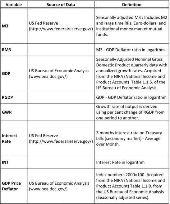
1. Table 1. The Definition and Sources of Data 63

2. Table 2. Unit Root Tests 64

3. Table 3. Estimation of the Error Correction

Money Demand Model 65

4. Table 4. Chow Test Results 66

5. Table 5. Short Run and Long Run Elasticites of Money Demand 66 6. Table 6. Comparison of the Estimated Long-Run Elasticities 67 7. Table 7. Estimated Parameters of the Model 69 8. Table 8. Estimated Welfare Cost of Inflation 69

LIST OF FIGURES

1. Figure 1. Graphical Representations of RM3, RGDP,

CHAPTER I

INTRODUCTION

Several articles have attempted to understand the behavior of the money demand and empirical studies have been carried out in order to derive monetary policies leading the economy. As Gillman and Otto (2002) suggests the money demand has to be analyzed since interest elasticity of money demand plays a crucial role for the key issues of macroeconomics, such as hyperinflation, the cost of inflation policy and growth rates of the economy. Considering the literature on money demand, the articles are generally divided into two parts depending on their organization. First type of articles develop an insight into the theoretical side of the problem, which is then supported by empirical tests. The second type of articles are purely empirical, these start with a simple quantity theory of money and run the money demand regressions. Both parties emphasize significant problems as dealing with the money demand, which have to be integrated in order to develop a better fitted model for the money demand. Even though each article follows a

different way related to its aim, basic obstacles have to be revisited to model the money demand combining the theory and empirical study.

This thesis is basically a theoretical study of the long run-short run demand for money including an empirical model for the US. Money demand is motivated by a cash-in-advance constraint placed upon the purchase of all real goods. Financial transactions, which can be viewed as ‘trips to the bank’1 are determined by a production function. The transactions technology includes a fixed and a variable input where in the short run the consumer can only change the variable input and in the long run the fixed input can also vary. The innovation of this thesis is the inclusion of this fixed input, which represents things like the number of bank branches, ATM machines, the types of bank accounts offered by banks, the consumer’s knowledge of available banking options, etc within a dynamic framework. The fixed input is considered as the ‘bricks-and-mortar’ of a bank. On the other hand, the variable input denotes the variable effort that the consumer and banks put into transacting: Baumol’s (1952) concept of ‘shoe-leather’. In order to test our theoretical insights quarterly US Gross Domestic Product (GDP), growth rate of GDP, interest rate and M3 money demand from 1959:1 to 2006:4 are used in an Error Correction Model. It is found out that the empirical results utterly support the forecasts of theoretical model.

1 _{The model is abstract and does not include a formal banking sector. ‘Bank’ refers to the}

This thesis contributes to the literature with its theoretical framework, which is supported empirically. From the theoretical side, a Cash-in-Advance (CIA) model is used since CIA model captures the transactions demand of money2. The presence of a fixed input in CIA model provides a structure for analyzing innovation in the technology of transactions, a micro foundation for price stickiness and has implications for the time-dynamic of the welfare cost of inflation. Depending on the simplified money demand functions of the theoretical model, the empirical model relies on the standard log-linear form. However, other studies in the literature either focuses on only theoretical or empirical part or starts to investigate the empirical problem without correctly linking to the model. In Chapter II the innovations made in this thesis are discussed in more detail.

Implementing this model, it is found out that (i) the share of the fixed input in producing transactions technology, in other words the relative productivity of the fixed variable, affects the short run interest elasticity of demand for money, but not the long run. Larger values of this share increase both the response of money to interest rates and output in the short run. On the other hand, the long run interest rate elasticity depends only on the consumer’s elasticity of substitution between consumer good and real balances (ii) the interest elasticity of money demand is a multiple of the income elasticity of money demand in short run (iii) the consumer’s elasticity of substitution

2 _{CIA model means that in an economy the consumer’s purchase will be limited by the cash}

between consumer good and real balances affects the short run elasticities of money demand together with the share of fixed input (iv) The short run interest elasticity of demand for money is less elastic than the long run demand; the short run output elasticity of money demand is more elastic than the long run. This apparent dichotomy is explained by the differing roles of income and interest rates in the demand for money. An increase in income forces an increase in equilibrium spending, causing the consumer to hold more cash and to transact more often in the long run. In the short run the consumer holds relatively more cash since there is a fixed input into creating transactions. In contrast, an increase in the interest rate provides an incentive to hold less cash and therefore to transact more often in the long run. In the short run, the existence of a fixed input into transacting restricts the consumer’s ability to substitute transactions frequency with the level of cash balances (v) Empirical evidence from quarterly US data verifies the theoretical forecasts on the direction of the relation among monetary variables. The unit income elasticity in long-run can not be rejected. The interest and output elasticities imply higher share of fixed input and low elasticity of substitution between the consumer good and real balances. Besides, the welfare cost of inflation is quite high for the US (vi) Lastly, the formula found for optimal prices in long run confirms the P-Star3 approach and accepts the use of price gap as an indicator for changes in inflation for the US.

3 _{P-Star concept was a popular topic in economics in 1990’s following its introduction with}

the study of Hallman, Porter and Small (1989; 1991). This view is based on the simple quantity theory of money in order to explain sticky prices. In chapter II the definition and evaluation of P-Star approach is discussed in more detail.

This thesis is organized as follows; section 2 revisits the literature on money demand; section 3 introduces the theoretical model together with the solutions for long run and short run including the welfare cost of inflation and P-Star approach; section 4 explains the empirical model used to verify theoretical insights and summarizes the empirical findings; lastly, section 5 presents a brief conclusion.

CHAPTER II

LITERATURE SURVEY

The literature on money demand includes several articles. Most of these studies concentrate on the interest and output elasticities of money demand because of the role of these sensitivities in macroeconomic policies. As emphasized in Chapter I, these studies can be grouped in two parts; articles on theoretical modeling and articles on empirical investigation. The need of combining regressions with the theory arises as a consequence of the need to acquire better fitted models. The motivation of this thesis is to model an economy that draws out actual implications.

The theoretical and empirical methodologies of this thesis have superiorities compared to the literature. The important innovations of this thesis can be grouped as follows:

i. Articles starting with a theoretical vision basically have conceptual problems such as inclusion of one variable within the utility function

or not. These articles choose various methods to handle the money demand, but whenever the aim is to construct a consistent micro founded model, Cash-in-Advance (CIA) model is a better method to have money within the model. First reason is the simple way of inserting the money into dynamic model (Duca and Vanhoose, 2004). Rather than other complicated models, such as money-in-the-utility function (MUIF) or dynamic inventory-theoretic model, Duca and Vanhoose (2004) claim that the CIA models are popular for the sake of practice. Another study by Stockman (1989) underlines the significant superiority of the CIA over alternatives to evaluate the transactions demand for money. Our second reason to adopt CIA model is that in this thesis a different generalized version of CIA constraint including the velocity of money is introduced. Even though the models of Lucas (1980), Lucas and Stokey (1987) and Corbae (1993), where velocity exits in the CIA model with different properties but with limitations on the velocity of money, the flexibility of the trade-off between cash holdings and transactions activity can not be provided. Therefore, in this thesis CIA model allowing same trade-off is adopted but a time dynamic formulation is made including a fixed and variable input into the transactions technology. Thirdly, as an extension of the Baumol-Tobin model, CIA model can be used to shed light on effects of such non-steady-state events, like open market operations, when the main aim would be to

capture the transactions demand for money to derive policy implications. Nevertheless, MUIF, which is nearly same as CIA theoretically, can be accepted as an alternative method as long as the measurement of how important the liquidity services for an agent is the core of the study (Holman, 1998). Nevertheless, MUIF is criticized because it is the service that provides utility rather than money itself.

ii. The studies focusing only on the empirical side of the money demand to forecast and/or understand the past movements of the relation among monetary variables do not provide reliable and robust results. The reason is that without models, the choice of functional forms, independent variables or the adaptation of different techniques can make the results more sensitive to these parameters, so conclusions may be misleading. As analyzing the effects of a change in the economy, such as a political or worldwide economic change, pure empirical studies start with simple quantity theory of the money demand. Ball (2001) takes the log-linear form of the theory to analyze the US postwar and prewar period; Beyer (1998) includes short-run and long-run of interest rates in the model for Germany. Nevertheless, these studies are lack of fitted theoretical models. The claims of these studies rely utterly on the regression results. In fact, empirical studies experience important problems related to the data. Firstly, especially after the arise of the

‘missing M2’ in the US4, the question of the monetary aggregation became a question. Different explanations are proposed to explain missing M2. The study of Peltzman (1969) drew attention to the future research for the trend term since the changes in velocity could not be explained only with interest rates, income and limited definition of money demand. Studies investigating missing M2 found out not only problems related to the omission of the other financial assets in the restricted definition of the money demand, but also considerable effect of change in asset transfer costs. Indeed, Duca (2000) explains the missing M2 completely with the change in asset transfer costs rather than omitted variables from the money demand definition. However, incorporation of the other financial assets is a necessary condition since the cross price elasticities of other financial assets is considerably high where these values are calculated in Collins and Anderson (1998) for the US. Melnick (1995) shows that the financial services have to be included to enhance money demand in order to derive a stable money demand and long-run relationship between the variables for Israel. On the other hand, Mehra (1993) points out a stable relation for M2 demand for the US adopting an Error Correction Model (ECM). Another study by Hallman, Porter and Small (1991) investigates a long-run link between M2 and price level. Other studies by Beyer (1998), Ericsson

4 _{The ‘missing M2’ refers a significant rise of M2 growth and considerably a low increase in}

and Sharma (1998), Lütkepohl and Wolters (1998), Brand and Cassola (2000), and Kontolemis (2002) include the M3 definition of money to acquire a stable money demand. Even though controversial studies exist, the literature points out that the common view is to use a broad definition of money demand not to exclude any explanatory power. Therefore, this thesis uses the definition of M3 that incorporates M2 and large time Repos, Euro-dollars, and institutional money market mutual funds. Despite the release of the US Federal Reserve (2005) claiming that “M3 does not appear to convey any additional information about economic activity that is not already embodied in M2 and has not played a role in the monetary policy process for many years”, M3 definition is selected to prevent data loss and enclose all ‘money supply’. Secondly, the form of money demand function plays a crucial role. Mehra (1993) adopts an ECM to start the regressions where Hafer and Hein (1984) choose a simple linear regression in order to evaluate the income and interest rate elasticities of money demand. Cuthbertson (1997) clarifies the rising performance of the regression as the inclusion of lagged dependent variable. The results proving that most assets adjust slowly verify the use of ECMs (Cuthbertson, 1997). Inclusion of the lagged value of money demand is reasonable to include the effect of past movement of money demand on the current level. This makes ECM more realistic motivating us to adopt an ECM.

iii. This thesis revisits not only simple money demand model but also the P-Star within the framework of both theoretical and empirical model. Though this thesis does not purely concentrate on P-Star, the point is that we can derive sticky prices instead of assuming them as in P-Star. Historical root of the P-Star view was the core of many studies apart from the money demand research left in the 20th century. The P-Star model arises from the quantity theory of money:

. .

M V =P Y that relates the money supply (M), nominal income (Y) and velocity of money (V). In the long run equilibrium if we will substitute the potential levels of each variable, we obtain:

. * *. *

M V =P Y that summarizes a stable money demand relation. Solving this equation for P* shows that any change from the potential prices can be rewritten in terms of an output gap plus a velocity gap. Besides, a change in inflation would be a function of price gap, ( *P −P), since a gap from the long run equilibrium would force prices to return to the equilibrium level. Humphrey (1989) explains that this price gap draws the path of inflation. The underlying idea of P-Star is the lagged price response leading to arise of price gap (Humphrey, 1989). Nevertheless, this model is meaningful as long as the money supply and income are exogenous to the model (Beyer, 1998). Hallman, Porter and Small (1989; 1991) introduced the concept of P-Star over the US data claiming that the price gap can be an indicator for the inflationary pressure for the US.

Other studies on different countries (Tatom, 1992; Hoeller and Poret, 1991; Kole and Leahy, 1991; Atta-Mensah, 1996) confirm the use of P-Star model. The studies on the Euro Area also support the P-Star view (Gerlach and Svensson, 2001; Scharnagl, 2002). Another study by Riemers (2001) over 110 countries, including OECD and Latin America countries, verifies the cointegrating relation among the actual prices and an equilibrium price level termed P-Star. Because the P-Star model is based on assumption of a stable money demand and stationary price gap, the studies on P-Star model proves out that a stable long term money demand function exists and P-Star model has significant power to explain the path of inflation. The solution of our theoretical model derives an equation for the optimal prices in the long run, p*, that links our theoretical model to the P-Star. Besides, the empirical model embraces the test of P-Star for the US data.

iv. The dynamic construction of our theoretical model must be underlined because inclusion of a time element enables us to calculate long run and short run elasticities separately changing over time. Besides, the welfare cost of inflation is also derived in a time varying formula. Other studies following empirical road such as Mehra (1993) or Hafer and Hein (1984) calculates only static long run elasticities of money demand. Nevertheless, there are only few studies distinguishing long run and short run elasticities via time

varying theoretical and/or empirical models.

The content of this thesis combines the theoretical and empirical investigation. Considering the literature, the theoretical model with the careful integration of a fixed input into transacting and empirical tests on the US data together with reference to the P-Star model and dynamic welfare cost of inflation make this thesis significant. The importance of the money demand to enhance policies motivates our study of a better fit money demand model.

CHAPTER III

THE THEORETICAL MODEL

5

Our theoretical model consists of only government and consumer. The economy is a pure consumption ‘tree economy’. The consumer faces a cash-in-advance constraint upon all purchases and maximizes utility subject to budget and cash-in-advance constraints. The government makes transfer payment financed by the creation of money and issues one-period bonds in order to compensate the debt. The transactions technology is defined in terms of a Cobb-Douglas type of production function. Output evolves according to the function y′= ⋅γ′ y where γ is a stochastic growth parameter and y represents the output6. We focus on the properties of the long run - short run income and interest rate elasticities of money demand.

5 _{The theoretical model is derived by Dr. Neil Arnwine.}

6 _{Time subscripts have been dropped for clarity. A prime denotes variables evaluated at time}

3.1 The Government

The government provides flat rate transfer payments to consumers, which is equal to the money creation. The money supply evolves according to;

M

M′=ω⋅ where M denotes the money supply and ω is the growth rate of money supply7. Government debt in the form of one period discounted bond is included in the model to formalize the market interest rate. Without the loss of generality we can assume thatB′=B=0, meaning that these bonds are supplied in zero amount.

3.2 The Transactions Technology

The theoretical innovation of this thesis is the inclusion of the fixed and variable inputs in the transactions technology modeling. Transactions are produced using a constant return to scale Cobb-Douglas production function in the two inputs τ and k:

1 1 1 ( , ) ( ) n k k y ψ φ φ ψ τ ₌θ τ − − − ₍₁₎

where τ is a variable input and the input k is fixed in the short run. The transactions technology is homogenous of degree 0 in k, τ, and y, so that an increase in output, together with a proportional increase in the transacting inputs has no effect on the number of transactions per consumer. Therefore, the results are invariant to the units of measurement for income. The parameters θ>0 and 0≤φ≤1 determine the absolute and relative

productivity of the two transacting inputs. ψ is a parameter that demonstrates the customer’s elasticity of substitution between the real goods and real balances.

The fixed input evolves in the standard way:

(

)

k x

k′= 1−δ ⋅ + (2) where δ is the rate of depreciation and x is investment into the fixed input. Resources used up in transacting cannot be consumed so there is a resource constraint of:

y x

c+τ+ = (3) where c denotes the consumption.

The expenditure of τ and/or x allows the consumer to reduce the level of real balances held, at the cost of forgone consumption. The variable input can be thought of as ‘shoe-leather’ costs of transacting while the fixed input can be considered as ‘bricks-and-mortar’ costs. The fixed input includes tangible physical assets, such as the number of bank branches and ATM machines, as well as knowledge and human capital, represented by the variety of banking services and the consumer’s knowledge of the availability of these services. As in Baumol-Tobin model, the consumer faces a trade-off between supplying these inputs versus holding average cash balances.

3.3 The Consumer

The representative consumer maximizes the utility given by;

( )

1 , ln 1 , 1 1 ₁ = α = ≠ α ⋅ α − = −α c c c u (4)

where α is the parameter and u(.) denotes the utility function of the consumer. The utility function is assumed to be a constant returns to scale.

A representative consumer is subject to the following budget constraint:

(

c x

)

M

( )

i B P y M B

(

)

M

P⋅ +τ + + ′+ 1+ −1⋅ ′≤ ⋅ + + + ω−1 ⋅ (5) The right-hand side represents the consumer’s wealth, consisting of, moving from left to right, current income, money balances carried into the period, maturing bonds, and a lump sum transfer payment from the government that equals money creation. The consumer divides this wealth between; again from left to right, current expenditure, carrying money balances into the next period, and discounted nominal bonds. The current expenditure items in the first term consist of consumption, shoe-leather expenditure, τ, and purchase of the fixed transactions input, x.

There is a cash-in-advance constraint placed upon the purchase of all real goods8:

(

+τ+

)

≤ ⋅

( )

τ ⋅ c x M n k,

P ₍₆₎

8 _{If the CIA constraint were placed upon the purchase of consumption goods only, this}

where M is the level of real balances obtained in a transaction and n is the number transactions in which the consumer obtains this amount of cash within the observation period. The formulation of equation 6 has a considerable difference than the other existing CIA constraints, because this constraint points a time dynamic analysis including fixed and variable inputs into the transaction technology. One explicit result of the analysis will be to show that n is the velocity of money. Omitting the n function in this model would be to implicitly assume that the velocity of money is constant at one. Studies have attempted to overcome the restriction on velocity by assuming that the cash-in-advance constraint only applies to a subset of transactions (Hodrick, Kocherlakota and Lucas, 1991) or by introducing a precautionary motive for holding money (Lucas, 1980; Svensson, 1985). The notion of velocity introduced in this thesis can be viewed as a generalization of Baumol’s (1952) model. Baumol’s model is generalized in three ways; first, the prices and interest rates are determined within the model instead of given exogenously; second, the model is time-dynamic rather than static; lastly, there is a fixed as well as a variable input into creating transactions.

In order to make the problem stationary, through dividing equations 5 and 6 by next period's money supply, M′, define the following: , ,

M B b M P p ′ ′ = ′ ′ = and M M m ′ ′ =

[

]

( )

ω − ω + + + ⋅ = ′ ⋅ + + ′ + + τ + ⋅ − 1 1 i 1 b p y b m m x c p (7)

where the term ω

− ω 1

represents the lump sum transfer of new money

creation to the consumer. The CIA constraint becomes:

(

)

⋅

( )

τ ω = + τ + ⋅ c x m nk, p . (8) Since consumption is valued both constraints will always bind in equilibrium.

3.4 The Value Function

The representative consumer’s problem can be expressed as a value function problem:

( )

S

{

u

( )

c Ev

( )

S

}

v k b m c ′ ⋅ β + = ′ ′ ′ τmax, , , , ₍₉₎

where β is the discount factor. The vector S =

{

k,ω,y

}

represents the state of the economy. The consumer’s problem is to select c,τ,m′,b′,k′subject to equations 7 and 8. Each period the consumer decides how much to consume, the number of trips to bank, the money balances and bonds will be carried to the next period, and the amount of fixed variable in the next period. In order to acquire the long run and short run equilibrium, we focus on the equilibrium conditions in the following section.

3.5 Equilibrium Conditions

money demand and the real goods market clears: 1

m′ = =m and c+τ+x= y (10) The first-order conditions derived from the maximization of value function are listed in Appendix A9. The combination of these first-order conditions with equation 10 gives the Euler Equations.

3.6 Long Run Stationary (Risk-free) Equilibrium

The closed form solutions for the model’s endogenous variables are found for the risk-free stationary equilibrium. The case in which the growth rates of output and money supply are constant, ω′=ω, γ′=γ, is considered. It is assumed that in a stationary equilibrium the income shares of the consumer’s choice variables should be constant and the number of transactions per period should also be constant over time. So, we guess that the following constraint has to be satisfied, and later confirm the guess:

n n y c y c y y y k y k _{= = ′=} ′ ′ = = ′ ′ = = ′ ′ , , , τ τ γ γ γ (11)

Solving the Euler Equations together with equation 11 gives the following result: . k τ = Θ where

[

β

(

δ

)

γ α

]

φφ ⋅ − − − − − = Θ 1 1 1 (12)

The term ‘Θ’ denotes the ratio of variable input to fixed input. The term

within the brackets,

[

β−1−

(

1−δ

)

γ−α

]

, is the net, after depreciation and correcting for capital accumulation due to the population growth, rate of return to the capital input. The ratio of shoe-leather to the fixed input depends on this rate of return and the relative productivity of τ to k, given by φ.

For the long run equilibrium the optimal prices, velocity of money, and the money demand functions are:

(

)

ψ φψ ψ −       ⋅ φ − ⋅ ψ − ψ ⋅ Θ ω θ = i y p 1 1 1 (13) n y p M y P V ≡ ⋅ =ω = (14)

(

)

i y p P M L _ ⋅      ⋅ φ − ⋅ ψ − ψ ⋅ Θ ⋅ θ = ω = ≡ ψ − φψ − ψ ₁ 1 1 1 (15)

The transactions technology is proved to be the velocity of money in equation 14. The money demand function in equation 15 can be viewed as a generalization of Baumol’s (1952) model. The important changes are, as emphasized in section 3.3: the model is in general equilibrium with the price level and the interest rate determined within the model, and the problem is time-dynamic rather than static.

Taking the partial derivative of equation 15 with respect to income gives the long run output elasticity of money demand:

1 = ⋅ ∂ ∂ = L y y L LR Ly ε (16)

The long run income elasticity is unity as expected. Arnwine (2007) demonstrates that only a unitary income elasticity of money demand is consistent with the notion of admissibility for a standard CIA model.

The long run interest elasticity of money demand is derived in equation 17. ψ ε ⋅ =− ∂ ∂ = L i i L LR Li (17)

The long run interest elasticity of money demand is just the negative of the consumer’s elasticity of substitution between the consumer good and the level of real balances. As expected the link between the money demand and interest rates is negative.

3.7 Short Run Equilibrium

In short run two assumptions are made to simplify the results. First, k is viewed as completely fixed in the short run and any response of money demand to a change results from changes in variable input, τ, only. Second, it is assumed that any response begins from a position of long run equilibrium allowing us to substitute in the long run expressions for τ, k, L and n to simplify the derived expressions. Solving the money demand function by using equation 1:

(

_τ

)

−−ψψ ⋅ −ψ ⋅ θ = = ⋅ ω = ≡ − φ −φ 1 1 1 1 1 1 y k n y p P M L (18)

The short run money demand responds to changes in interest rate and income via a change in the variable input because k is assumed to be fixed. Contrary to the closed form solution of long run, an indirect function (equation 20) is constructed by using equation 19 in order to evaluate the responses of τ with respect to income and interest rate. The equilibrium interest rate is:

ψ − − ψ −φψ − ψ − φψ τ ⋅ φ − θ ⋅ ψ ψ − = 1 1 1 1 1 1 1 y k i (19)

The indirect function is:

(

)

1 0 1 , , 1 1 1 ₌       ⋅ θ φ − ⋅ ψ − ψ − τ = τ ψ − − φψ − φψ _{y i} k i y F (20)

Taking the total derivative and setting equal to zero:

(

τ,y,i

)

=F_τ⋅dτ+F ⋅dy+F ⋅di=0

F

d _{y i} (21)

Rearranging, we obtain the partial derivatives:

i y k i F F di d _i ⋅      τ ⋅       ⋅ θ φ − ⋅ ψ − ψ ⋅ φψ − ψ − = − = τ −ψ φψ τ 1 1 1 1 1 (22) y F F dy d y _⋅ τ φψ − = − = τ τ 1 1 (23) We can then find the short run interest elasticity and output elasticity for τ, the shoe-leather expenditure.

k y i i di d SR i  ⋅Θ ⋅      ⋅ θ φ − ⋅ ψ − ψ ⋅ φψ − ψ − = τ ⋅ τ ≡ ε −ψ φψ− τ 1 1 1 1 1 1 (24) φψ τ τ ετ ≡ ⋅ = ₋ 1 1 y dy d SR y (25)

interest rate causes an increase in the shoe-leather expenditures. Besides, the response of τ to income depends only the relative productivity of inputs and substitution between consumer goods and real balances. On the other hand, interest rate sensitivity is a function of the levels of income and fixed input. Because we are assuming that the fixed input does not vary in short run, the level of income affects τ via not only equation 25 but also equation 24.

Returning to the short run money demand function, we can express the response of money demand to interest rates and output in terms of τ’s response. φψφ ε ψ φψφ τ τ ε − − = ⋅ − − − = ⋅ ∂ ∂ ⋅ ∂ ∂ = ⋅ ∂ ∂ ≡ 1 1 . 1 1 LR Li SR Li L i i L L i i L (26) 1 1 1 _> − = ⋅       ∂ ∂ + ∂ ∂ ⋅ ∂ ∂ ≡ φψ τ τ ε L y y L y L SR Ly (27)

In short run the elasticity of interest rate is proportional to elasticity of income. The reason is that the short run sensitivity of shoe-leather expenditure to interest rate is also affected by the level of income. Comparing the short run and long run elasticities, money demand is more interest inelastic in the short run because the consumer can not easily change the velocity in the short run due to the fixed input. The degree of short run rigidity

depends on the share, φ, of the fixed input, k, in producing transactions, n, in equation 1. As φ approaches 0, there is no fixed input, then interest and output elasticity of money demand are the same in the short run and long run. As φ approaches 1, the interest elasticity of money demand becomes perfectly inelastic in the short run and income elasticity of money demand becomes larger in the short run.

3.8 Welfare Cost of Inflation

The welfare cost of inflation can be interpreted as the increase in income to compensate the welfare cost due to inflation because a rise in prices would reduce the amount of consumption, so the utility.

In our model, in line with Bailey (1956) and Friedman (1969), the welfare cost of inflation is derived by the indirect utility function. A unit-free measure of the welfare cost of inflation is the elasticity of welfare compensating income with respect to changes in the nominal interest rate. This is calculated by totally differentiating the indirect utility function, setting the utility change equal to zero, and then solving for the interest elasticity of compensating income. The difference of our results is that there is a time element to the welfare cost of inflation. The welfare cost does not have a static but has a dynamic formulation.

Long Run:

In the long run the indirect utility function, as a function of the interest rate and output level, is derived as following:

( )

[

]

(

)

α α ψ φψ φψ α θφ ψ ψ δ α δ τ α − − − − − ⋅               ⋅ − ⋅ − ⋅ Θ + Θ − ⋅ − = − − ⋅ − = 1 1 1 1 1 1 1 1 1 1 1 1 , y i k y y i uLR (28)

The optimal inflation rate is found when the nominal interest rate is zero. Using equation 28 it can be found how much additional income is needed to receive to compensate for the welfare cost of inflation. Differentiating the equation 28 to acquire the elasticity of inflation compensating income with respect to the nominal interest rate:

( )

dy y U di i U dy y U di i U y i U d ⋅ ∂ τ ∂ ⋅ τ ∂ ∂ + ⋅ ∂ τ ∂ ⋅ τ ∂ ∂ = ⋅ ∂ ∂ + ⋅ ∂ ∂ = , (29)

(

)

(

)

[

(

)

]

(

)

[

]

ψ

(

φψ φψ

)

[

(

)

]

ψ ψ φψ φψ φ ψ δ ψ θ φ ψ δ ψ ε ₋ − ₋ − ₋ = ⋅ − − Θ +Θ ⋅ − ⋅ ⋅ − ⋅ ⋅ Θ + Θ ⋅ − − = ⋅ = _{1 1 1} 1 1 0 1 1 1 1 i i y i di dy du LR yi (30)

In the long run the welfare cost of inflation depends on the level of interest rates, growth rate of output and other parameters of the model including the absolute and relative transaction function’s productivity parameters, the output growth rate, the consumer’s time discount rate, and the depreciation rate for the fixed factor.

Short Run:

derivative of the indirect utility function and setting equal to zero, while keeping k fixed at its equilibrium level. The indirect utility function for short run is given in equation 31:

( )

_⋅

[

_−τ−δ

]

−α α − = 1 1 1 ,y y k i U (31)

Taking total derivative and setting equal to zero:

( )

[

]

[

]

dy y k y di i y k i k y dy y U di i U dy y U di i U y i U d ⋅ ⋅ − ⋅ − − + ⋅ ⋅       ⋅       ⋅ − ⋅ − ⋅ − − ⋅ − − − = ⋅ ∂ ∂ ⋅ ∂ ∂ + ⋅ ∂ ∂ ⋅ ∂ ∂ = ⋅ ∂ ∂ + ⋅ ∂ ∂ = − − − τ φψ δ τ τ θφ ψ ψ φψψ δ τ τ τ τ τ α φψ ψ α 1 1 1 1 1 1 , 1 (32)

Then, the interest elasticity of inflation compensating income is:

(

ψ

)

ε = ⋅ =− − = 1 0 du SR yi y i di dy (33) The welfare cost of inflation in short run is a function of only the substitution between the consumption goods and real balances. An increase in the inflation rate in short run is quite beneficial because it causes the consumer to hold more money and transact less often, yielding higher equilibrium consumption. In the long run an increase in the inflation reduces welfare as consumer increases the fixed input transactions. The increase in the fixed input reduces consumption in equilibrium as more capital must be replaced and because the variable input into transactions is proportional to the fixed input.

3.9 P-Star and Endogenous Sticky Prices

As referred in Chapter II, P-Star approach claims that a stable money demand relation in equilibrium would be summarized as follows:

* * * MV P Y ≡ (34)

where P is the prices, V the velocity of money and Y is the income. ‘*’ denotes the equilibrium levels and capital letters denote the nominal values. Equilibrium prices are determined with respect to Equation 34.

Returning on our model, the equation for the long run equilibrium price levels is introduced in equation 13. Remembering this equation:

( )

(

)

ψ φψ ψ φ ψ ψ ω θ       ⋅ − ⋅ − ⋅ Θ = ∗ ∗ ∗ ∗ − ∗ _i y p 1 1 1 (35)

The optimal prices are a function of several parameters, including the elasticity of substitution between the consumer goods and real balances, absolute and relative productivity of fixed and variable inputs. Assuming that ψ , φ, θ, β, δ , γ−α and ω∗ are constant for the long run solution, price changes depends on income level and interest rates. The equation determining the long run interest rates from Appendix A is given below10:

( )

−ψ −φψ

(

)

ψ       ⋅ φ − ⋅ ψ − ψ ⋅ Θ ⋅ θ = τ i k n 1 1 , 1 (36)

Solving for interest rate, equation 36 implies that interest rate is a function of

10 _{This is the equation 32 in Appendix A.}

the velocity of money, n. By combining equation 35 and 36, the change of prices is a function of only income and velocity of money:

* ( *, *)

p f y v

∆ = ∆ ∆ (37)

The prediction of our model encompasses what the P-Star approach predicts. The model confirms that the price gap is a function of the velocity and income gap. Nevertheless, the basic difference comes from the other variables ψ , φ, θ, β, δ , γ−α and ω∗that are assumed to be constant. Therefore, the simple summation of income and velocity would not add up to price gap, but a multiple of these gaps would add up to the price gap.

In brief, our theoretical model includes the view of P-Star with some generalizations:

i. The price stickiness arises from the prices that are endogenously derived within the model. The prices are not exogenous.

ii. The price adjustment does not take place with the simple summation of change in income and velocity. The gap in prices depends on other parameters of our theoretical model.

CHAPTER IV

EMPRICIAL MODEL

11

The theoretical model presented in Chapter III claims that the money demand is a function of income, interest rate and the growth rate of income as well as the other parameters of the model. To simplify our regressions and acquire the income and interest rate elasticities in order to compare with the theoretical counterparts the money demand function is regressed on income, interest rate and growth rate of income. An error-correction model, which enables us to relate the movement of the variables to the previous period's gap from long-run equilibrium in a dynamic framework, is adopted. The P-Star approach is tested and welfare cost of inflation is estimated within this framework.

4.1 The Data

The error correction model for money demand is estimated using quarterly

data from 1959 Q1 to 2006 Q4. Gross domestic product and GDP price deflator12 are obtained from the US Bureau of Economic Analysis, and interest rate and money supply are acquired from the US Fed Reserve. GDP Price Deflator is used to convert nominal values to real balances13. The rate on 3 months Treasury Bills is selected to represent the opportunity cost of money. The term of Treasury bill is chosen as three months in order to capture short term effects. Growth rate of output is derived using per cent change of RGDP from one period to another14. M3 is used as the money supply15. GDP, GDP price deflator and M3 are selected from seasonally adjusted time series so that dummies to capture cyclical effects are not needed.

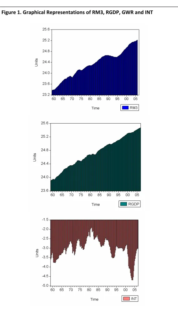
The graphical representation of the variables given in Figure 1 indicates that there is not any significant break point implying that unit root tests can be applied. The graphs of RM3, RGDP and INT rise with the time indicating these variables can be non-stationary. On the other hand, the plot of GWR refers that GWR is integrated of order zero.

12 _{The GDP price deflator is the ratio of nominal GDP in a given year to real GDP of that year,}

so measures the change in prices that has occurred between two years. This index gives a useful measure of inflation on all goods produced in the economy (Dornbusch and Fischer, 1994).

13 _{The Consumer Price Index is also used to convert nominal values to real values.}

Nevertheless, the ECM with GDP Price Deflator gives better results.

14 _{The definitions of the variables and details about the sources are presented in Table 1.} 15 _{The ECM is also constructed for M2 and M1, but the model with M3 perfectly reflects the}

Augmented Dickey Fuller (ADF) test results are summarized in table 2. Comparing the test statistics with the critical values, RM3, RGDP and INT are integrated of order one whereas GWR is integrated of order zero. Nevertheless, as suggested in Schwert (1989) and DeJong, Mankervis, Savin and Whiteman (1992) ADF test can suffer from size distortions in the presence of negatively correlated moving average errors. Even though there is no uniformly powerful test for unit root hypothesis (Stock, 1994), one solution to the size distortion problem of ADF can be to implement Dickey Fuller GLS test (Maddala and Kim, 2004). DF-GLS test results are also presented in table 2. Since inclusion of trend term plays a crucial role for the power and size of the unit root test and almost all macroeconomic variables show tendency to increase over time, it is more realistic to consider the case with intercept and trend term (Maddala and Kim, 2004). The results support that RM3, RGDP and

INT have unit root, and GWR is stationary in line with the visual test.

4.2 Empirical Specifications

Error Correction Model:

Following the parameters of theoretical model, our empirical model in form of an error correction model is given below:

1 2 3 4 3t t RM =β β+ RGDP+β INT+β GWR+E (38) 1 2 3 1 2 3 4 0 0 0 4 5 6 1 1 3 3 n n n t s t s s t s s t s s s s n s t s t t s RM RGDP INT GWR RM E U α α α α α α − − − = = = − − = ∆ = + ∆ + ∆ + ∆ + ∆ + +

∑

∑

∑

∑

A (39) where RM3 is real money balances, RGDP is real Gross Domestic Product (GDP), INT is the 3 months Treasury bill rate and GWR is the growth rate of RGDP. E and U represent the random disturbance terms. As used in previous papers in literature such as Ball (2001; 2002), Beyer (1998), Duca (2000) functional form of equations are derived in log linear form. RM3, RGDP and INT are in natural logarithms, Δ is the first difference operator and subscripts are the time indexes. Equation 38 is the long run equilibrium money demand function whereas the equation 39 shows the short run dynamics. β2 and β3 are the long run income and interest elasticity of money demand since the equation is in log linear form. In equation 39, αis (i=2,3,4,5) denotes the short run sensitivity of money demand with respect to income, interest rate, growth rate and past movements in the money demand, and α6 is the error correction

coefficient. Mehra (1993) suggests that the coefficients, αis, can be used to “measure the short-run responses of real M3 balances to changes in income and opportunity cost variables”. Other studies by Gillman and Otto (2002), Sriram (1999) and Choi and Oxley (2004) use the coefficients in the ECM to describe the short run dynamic model for money demand. Greene (2003) explains that these short run dynamics are the change of the related variable from the long run equilibrium path to denote the variation in dependent variable. Following this view, the long run elasticities are derived from equation 38 whereas equation 39 is used for a proxy for the short run elasticities of money demand.

As long as the variables in equation 38 are cointegrated, then the error correction form in equation 39 can be estimated implying that error correction coefficient is different than zero (Engle and Granger, 1987). Mehra (1993) suggests two alternative ways to estimate error correction form. First way adopts two step procedure of Engle and Granger (1987) based on the assumption of nonstationarity of all variables in equation 38. According to this approach, equation 38 is estimated by Ordinary Least Squares (OLS) to obtain the residuals. These residuals are substituted in equation 39 to estimate the short run dynamics. Nevertheless, as explained in the previous section, growth rate of output is integrated of order zero. Therefore, Engle and Granger (1987) approach is inappropriate. Alternative way to estimate equation 38 and equation 39 jointly is to substitute Et-1 from equation 38 and

rewriting equation 39: 3 1 2 1 6 1 2 3 0 0 3 4 4 5 6 1 0 1 6 2 1 6 1 6 4 1 3 3 3 n n t s t s s t s s s n n s t s s t s t s s t t t t RM RGDP INT GWR RM RM RGDP INT GWR U α α β α α α α α α β α β α β − ₌ − ₌ − − − − = = − − − ∆ = + ∆ + ∆ + ∆ + ∆ + − − − +

∑

∑

∑

∑

(40)

Unless the nonstationary variables in equation 39 are not cointegrated, equation 40 can be estimated (Phillips 1986; Sims, Stock, and Watson 1990). Then, the coefficients of equation 40 can be used to calculate the long run elasticities.

Equation 40 summarizes our empirical model. The link between the theoretical model and empirical model arises because α2 s,α3s are indicators

for SR Ly

ε and SR Li

ε , respectively. Also, β2 denotes the long run income elasticity of

money demand, LR Ly

ε , and β3 represents the long run interest elasticity,εLiLR.

The estimated values forα2s,α3s, β₂, and β₃ will be used not only for solving

elasticities but also for estimating the parameters of the model since elasticities were derived in Chapter III as a combination of simplified parameters. To illustrate; β3 would estimate the value of εLiLR =−ψ , α2scan

be used for solving

φψ ε − ≡ 1 1 SR

Ly and lastly, α3scan give an approximate value

for this expression ψ

φψ φ ε ⋅ − − − = 1 1 SR

Li . These estimated values can be used to

calculate the relative productivity of inputs (φ), or in other words the shares of the ‘shoe-leather’ and ‘bricks-and-mortar’ costs. Therefore, our empirical

model enables us to estimate, calculate and evaluate the theoretical model. Empirical Specifications for Endogenous Sticky Prices:

To test the P-Star approach the transformation in Beyer (1998) and Riemers (2001) is adopted. According to this transformation, rewriting equation 34 in logarithms: * * * m≡ p +y −v (41) * * * m p y v ∆ ≡ ∆ +∆ −∆ (42)

To determine v* the following long run money demand has to be estimated:

0

(m− p)=℘ − +y v u (43)

where v₀ is constant. Solving equation 43 with respect to (− − −m p y)=v and substituting ( *− m −p*−y*)=v* in equation 41:

0

* *

p = + −℘m v y (44)

Equation 44 gives the inverted money demand equation. Beyer (1998) and Riemers (2001) make a regression of equation 44 to test P-Star concept.

The difference between the studies of Beyer (1998) and Riemers (2001) and our empirical model is the existence of growth rate of output. The existence of interest rate does not cause a disparity because within the model the interest rate is also linked to the velocity of money, as proved in section 3.9. Hence, equation 43 is the restricted version of short run dynamics, equation 38. To test P-Star, we imposed the following restriction:

4 4 6 4 0 0 0 s β α α β = = =

for s=

{

1, 2,....,n₃

}

in equation 38 and 40 (45)

The coefficient test, not rejecting the null hypothesis of equation 45, is needed to confirm the P-Star approach. Unless the null hypothesis is rejected, p* would make sense. Then, the income would be exogenous in the long run not depending on (m−p). The theoretical model introduced in Chapter III predicts that P-Star approach would be verified with the coefficient test because interest rates and prices are determined within the model where the growth rate of output, γ , becomes constant in the long run and velocity of money is defined in terms a production function.

Causality between the Real Balances and Prices:

There is an ongoing debate between the money demand modeling perceptions of Friedman and Schwartz (1982) and Hendry and Ericsson (1991). According to the view of Hendry and Ericsson (1991) real balances are formulated as a function of other variables, including the price level, whereas Friedman and Schwartz (1982) choose to take money as exogenously affecting the change in prices.

In Chapter III we have seen that in our theoretical model the prices are endogenously determined; money supply evolves with the parameter ω. This theoretical framework leads us to the formulation of an empirical model, where prices would be determined within the model, so that money demand

would not be a function several parameters including prices. Hence, in our thesis we follow the way of Friedman and Schwartz (1982) to handle this causality problem.

In the next section estimation of empirical model, equation 40, by OLS is evaluated. In case of correlation between the independent variables and the disturbance term, error correction model also has to be estimated with instrumental variable (IV) method. Therefore, both OLS and IV regression results are considered.

4.3 Empirical Results

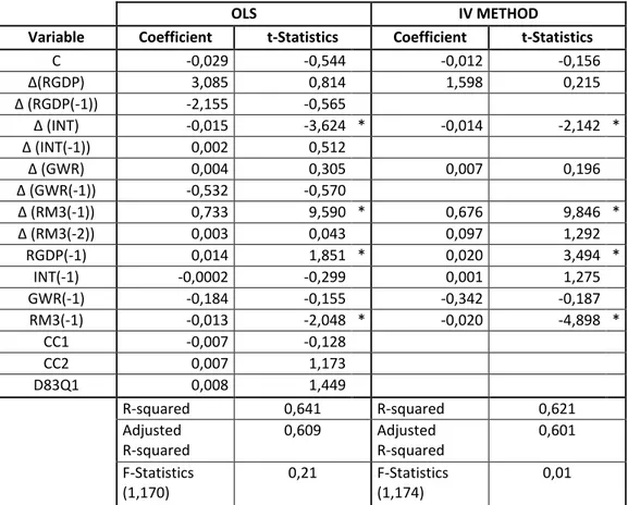
Table 3 summarizes the results of estimation of equation 40 with OLS and IV approach. As suggested in Mehra (1993) and Sill (1998), zero-one dummies are defined for Carter Credit Controls in 1982Q2 (CC1), 1980Q3 (CC2) and introduction of MMDAs and SuperNOWS in 1983Q1 (D83Q1).

Considering the results, the coefficients of INT and lagged ΔRM3, RGDP, RM3 are statistically significant. Joint significance test for coefficients verifies that all coefficients are jointly significant in both equations16. The signs of the coefficients are in line with the theoretical model17. There exists positive

16 _{The null hypothesis of “all coefficients are equal to each other and they are equal to 0” is}

tested. For IV approach F-statistics, F(10,174), is 321,803 and for OLS method F(16,170) is 51,575. The null hypothesis is rejected.

17 _{The OLS estimation is repeated after dropping the insignificant values of Δ (RGDP(-1)), Δ}

relation between money balances and output, whereas real money balances is negatively linked to interest rate as the theoretical model suggests. The dummies CC1, CC2 and D83Q1 are insignificant in OLS so these are not included in IV approach18. For OLS method the Durbin-Watson statistics is close to 2, and for IV approach Q-statistics of the model is low and insignificant indicating that there is no autocorrelation problem in residuals. Besides Q-statistics show that for the IV method selected instrumental variables are appropriate. For OLS estimation, the model explains about 64 percent of the variation in Δ(RM3) whereas 62 percent of variation is explained in IV approach. The coefficient of error correction term, α6, is significant and negative in both regressions. The significance of the coefficient validates the cointegrating relation. The negative sign implies that a fall in the excess money supply of the previous period leads to a rise in the cash holdings in the current period correcting to reduce the disequilibrium.

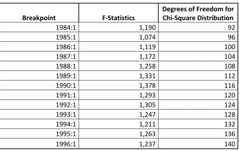
To test whether correct specification is selected to represent the theoretical model, Ramsey Reset test for stability is carried out for OLS estimation. According to the results nonlinear combinations of estimated values do not help to explain the changes in real money balances and the selected functional form is appropriate. Besides, the results for Chow’s Forecast Test

affected and the estimation performance of the regression is not developed these results are not listed.

18 _{IV approach is also applied with CC1, CC2 and D83Q1 but the dummies are found}

insignificant and the signs and significance levels of coefficients do not change. Therefore, IV approach is implemented without dummies. This insight is in line with Hafer and Jansen (1991), Mehra (1991) and Mehra (1993), where the dummies do not have a meaningful effect on the long run cointegrating relation for M2 demand function.

are summarized in table 4 for OLS method. The test confirms that there is no structural break.

Long run and Short Run Elasticities of Money Demand:

By normalizing the coefficients of RGDP (-1) and INT (-1) with the coefficient of RM3 (-1), the long-run income and interest elasticities are 1,073 (1,017) and -0,019 (-0,053), respectively (IV estimates are given in parenthesis). Comparing these long run elasticities with the short run values in table 5, the long run income elasticity of money demand is larger than the short run sensitivity whereas the interest rate sensitivity in long run is higher than the values for short run. Jointly test of summation of the coefficients of RGDP(-1) and RM3(-1) results that for both IV and OLS approach the null hypothesis of unit output elasticity of money demand cannot be rejected due to low F-statistics presented in table 3.

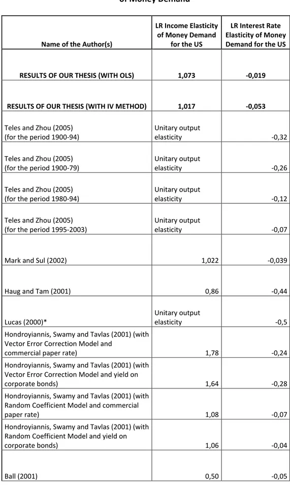
Table 6 proves that the income elasticities presented in table 5 are in line with the previous studies. The studies of Teles and Zhou (2005), Mark and Sul (2002), Lucas (2000), Hondroyiannis, Swamy and Tavlas (2001), Mehra (1991), Hafer and Jansen (1991), Lucas (1988), Hafer and Hein (1984), and Friedman and Schwartz (1982) find out an income elasticity of money demand near to 1 (In our thesis long run income elasticity is equal to 1,073 for OLS method and 1,017 for IV method). Only the studies Haug and Tam (2001), Ball (2001) and, for some intervals, Hafer and Hein (1984) are not close to 1. The estimation

method, selected time periods, form of the empirical model or selected variables can be reasons for these different values. Nevertheless, the common empirical and theoretical view is the unit output elasticity of income. Also, not only for the US but also several countries including Japan, the UK, France, Germany Mark and Sul (2002) claim that the unitary output elasticity is nearly one for time period 1957-1996.

The estimated interest rate elasticities in table 6 differ from one study to another. The most important observation is the dependence of the estimation of interest rate elasticity on the method, selection of the variable to denote interest rate and time period. To illustrate; Hondroyiannis, Swamy and Tavlas (2001) estimate -0,28 by using a vector error correction model, but -0,04 with the random coefficient model. Another example from the paper of Teles and Zhou (2005) point out that over the last decades the interest rate elasticity has dropped. Remembering that in our thesis the three months interest rate on Treasury bill is used as interest rate and time period is selected 1959-2006, we are not able to make one to one comparison. Our estimated interest rate elasticities are not contrary to the previous studies, but lower than most of the studies. The values of Hondroyiannis, Swamy and Tavlas (2001), Ball (2001), Mark and Sul (2002), and Teles and Zhou (2005) are closer to our estimations.

Estimated Parameters of the Theoretical Model:

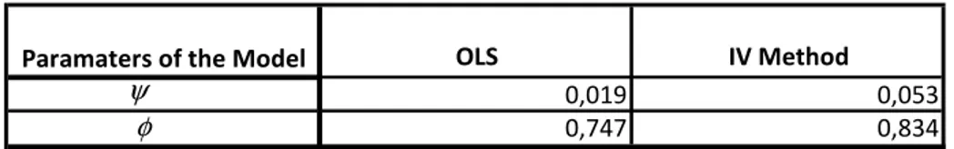
Combining the theoretical formulas for elasticities in equation 16, 17, 26 and 27 and the empirical findings, table 7 gives the values for parameters of the model. The consumer’s elasticity of substitution between the consumer good and real balances,ψ , is small (0,019 for OLS estimation and 0,053 for IV method) meaning that the consumer good and real balances are not close substitutes for the US over the selected period. The relative productivity of inputs to transactions technology, ф, implies that the contribution of fixed inputs is higher than of variable input for the US19. Therefore, the ‘bricks-and-mortar’ costs are larger than the ‘shoe-leather’ costs. Remembering that the fixed input includes tangible physical assets, such as ATM machines or number of bank branches, and human capital, it is meaningful to expect a higher share for the ‘bricks-and-mortar’ costs rather than variable input for the US where the investment in human capital and physical assets in banking sector is quite high20.

Estimated Welfare Cost of Inflation:

The estimated parameters of the model in table 7 indicates that the welfare cost of inflation, the elasticity of inflation compensating income with respect

19 _{The calculation of the parameter ф depends on both short run and long run elasticities of}

money demand. The solution of equations with respect to ф yield more than one solution, but a meaningful solution is presented in this thesis. Remember that the estimated values are included to give an insight about the precision of the theoretical model. The estimated parameters may not be equal to the precise actual values.

20 _{There is not any other study in the literature handling the transactions technology}

together with a variable and fixed input. Therefore, our results could not be compared with another benchmark paper.