Prediction and characterisation of intensity noise of ultrafast fiber amplifiers and low noise vibrometer for biological applications

(1)

PREDICTION AND CHARACTERISATION

OF INTENSITY NOISE OF ULTRAFAST

FIBER AMPLIFIERS AND LOW NOISE

VIBROMETER FOR BIOLOGICAL

APPLICATIONS

a thesis

submitted to the department of physics

and the graduate school of engineering and science

of bilkent university

in partial fulfillment of the requirements

for the degree of

master of science

By

Kutan G¨

urel

(2)

(3)

ABSTRACT

PREDICTION AND CHARACTERISATION OF

INTENSITY NOISE OF ULTRAFAST FIBER

AMPLIFIERS AND LOW NOISE VIBROMETER FOR

BIOLOGICAL APPLICATIONS

Kutan G¨urel M.S. in Physics

Supervisor: Assist. Prof. Dr. Fatih ¨Omer ˙Ilday July, 2013

We report on the experimental characterisation and theoretical prediction of intensity fluctuations for ultrafast fibre amplifiers. We formulate a theoretical model with which the intensity noise of a Yb-doped fiber amplifier can be pre-dicted with high accuracy, taking into account seed and pump noise, as well as generation of amplified spontaneous emission. Transfer of pump and seed sig-nal modulations to the amplified output during fibre amplification is investigated thoroughly. Our model enables design and optimisation of fiber amplifiers with regards to their intensity noise performance. As a route to passively decreas-ing the noise imparted by multi-mode diodes in cladddecreas-ing-pumped amplifiers, we evaluate the impact of using multiple, low-power pump diodes versus a single, high-power diode in terms of the noise performance. We use this gathered intu-ition on intensity noise to build a low noise fibre interferometer that is able to detect sub-5 nm vibrations for biological experiments.

Keywords: Fiber laser, Fiber amplifier, Relative intensity noise, Noise transfer function.

(4)

¨

OZET

ULTRAHIZLI F˙IBER Y ¨

UKSELTEC

¸ LER˙IN

KARAKTER˙IZASYONU VE S¸˙IDDET

G ¨

UR ¨

ULT ¨

ULER˙IN˙IN ¨

ONG ¨

OR ¨

UMG ¨

U VE D ¨

US¸ ¨

UK

G ¨

UR ¨

ULT ¨

UL ¨

U T˙ITRES¸˙IM ¨

OLC

¸ ER

Kutan G¨urel Fizik, Y¨uksek Lisans

Tez Y¨oneticisi: Assist. Prof. Dr. Fatih ¨Omer Ilday Temmuz, 2013

Bu tezde, ultrahızlı fiber yükselte¸clerin ¸siddet dalgalanmalarının deneysel karak-terizasyonu ve teorik öngörümünü sunuyoruz. Yb i¸ceren fiber yükseltecin gürültüsünü, tohum (seed), pompa (pump) ve kendili˘ginden olu¸san ı¸sımanın (ASE) gürültülerini de katkı alan, isabetli tahminde bulunabilen teorik bir model formule ediyoruz. Tohum ve pompa modülasyonlarının, yükseltilme sırasında sinyale transferlerini derinlemesine inceliyoruz. Modelimiz ¸siddet gürültü perfor-mansı a¸cısından, fiber yükselte¸clerin dizayn ve optimizasyonuna olanak veriyor. Kenar pompalamalı yükselte¸clerde kullanılan ¸cok modlu pompa sinyallerinin gürültülerinin pasif olarak dü¸sürülmesi i¸cin dü¸sük gü¸cte ¸cok sayıda pompa diy-odunun kullanımının yüksek gü¸cte az sayıda diyot kullanılmasına göre per-formans etkilerini de˘gerlendiriyoruz. S¸iddet gürültüsü konusunda edindi˘gimiz tecrübelerden yararlanarak, 5 nm genlikteki titre¸simleri algılayabilen dü¸sük gürültülü bir giri¸simci (interferometer) de˘gerlendiriyoruz.

Anahtar sözcükler : Fiber lazer, Fiber yükselte¸c, Göreceli ¸siddet gürültüsü, Gürültü aktarim fonksiyonu.

(5)

Acknowledgement

I’m grateful to Dr. Fatih ¨Omer ˙Ilday for making his laboratory available and the limitless opportunities he happily provided over the past 5 years.

I acknowledge the generous discussions I’ve had with ˙Ibrahim Levent Buduno˘glu, Co¸skun Ülgüdür, Kıvan¸c Özgören, Seydi Yava¸s, Hamit Kalaycıoglu, Parviz Elahi, Ç agrı S¸enel and Bastian Lorbeer. I thank all the previous and current members of the Ultrafast Optics & Lasers Group.

I would like to thank my committee members, Dr. Fatih Ömer ˙Ilday, Dr. Co¸skun Kocaba¸s and Dr. Mehmet Bur¸cin Ünlü for spending time on reviewing my thesis.

Finally I’d like to thank T ¨UB˙ITAK B˙IDEB for supporting me financially during my graduate study.

(6)

List of Figures

1.1 Structure of single clad and dobule clad fibers . . . 2

1.2 Schematic of a fiber amplifier . . . 4

1.3 Three level system . . . 5

1.4 Absorption and emission cross section curves for Yb+ _{ions. . . . .} ₆

1.5 Diagram of RIN measurement . . . 7

2.1 Single-clad fiber amplifier setup . . . 9

2.2 Double-clad fiber amplifier setup . . . 10

2.3 Experimentally obtained RIN curves of pump, seed, ASE and am-plified signals for single-clad amplifier . . . 11

2.4 Experimentally obtained RIN curves of pump, seed and amplified signals for double-clad amplifier . . . 13

2.5 Contour graphs of integrated RIN of amplified signal for seed signal center wavelengths of (a) 1030 nm and (b) 1060 nm for varying pump and seed powers . . . 14

(9)

LIST OF FIGURES ix

2.7 Integrated RIN values for combinations of multiple multi-mode

pump diodes . . . 16

3.1 MTF Measurement Setup . . . 18

3.2 Typical MTF curves . . . 24

3.3 MTF parameter for varying input modulation amplitudes . . . 25

3.4 MTF parameters for varying seed to pump power ratio . . . 26

4.1 Predicted RIN curves of pump, seed, ASE and amplified signals for single-clad amplifier . . . 28

4.2 Predicted RIN curves of pump, seed, ASE and amplified signals for double-clad amplifier . . . 29

4.3 Crosssection of Integrated RIN . . . 30

5.1 Fiber interferometer setup . . . 32

5.2 Interference fringes observed at the detector . . . 33

5.3 Observation of 4 nm amplitude kHz regime vibrations in the time and frequency domain measurements . . . 34

5.4 Diagram of Vibrational spectroscopy experiment . . . 35

B.1 LabVIEW Automated MTF and Vibrational Spectrescopy mea-surement design . . . 49

(10)

Chapter 1 Introduction

The most common application of fiber amplifiers is in the communications indus-try. The signals transmitted over long distances have to be preiodically amplified along the way to compensate for the losses. The noise becomes the major diffi-culty as it is amplified along with the signal. [1, 2, 3, 4]

Fibers amplifiers have found use in other industries as well. In particular, high-power fiber amplifiers are now used in laser material processing. [5, 6, 7] Very high output powers up to few kW’s has been reached. the noise becomes an important issue in material processing quality. [8]

However, despite its importance in various applications, intensity noise of fiber amplifiers has not received a close scrutiny. Recently, a systematic study of intensity noise of passively locked fiber lasers, operating in di↵erent mode-locking regimes was reported [9]. A key conclusion of this study was that there is often a trade-o↵ between the noise level of the oscillator and the highest pulse energy that can be extracted. Thus, the route to low-noise high-power operation could be to operate the oscillator at moderate power levels and amplify externally. The need for lowering the noise of fiber amplifiers, has motivated us to throughly characterize the noise of fiber amplifiers and build a formulation to predict it in order to optimize amplifier designs for performance.

(11)

Figure 1.1: Structure of single clad and dobule clad fibers

In addition, there are various applications where modulations of the signal or the pump need to be transferred to the amplified signal or an existing modula-tion to be preserved, such as carrier-envelope phase (CEP) stabilizamodula-tion [10], a necessity to construct stable optical clocks. We shine light into transfer of noise and modulation as well.

1.1 Fiber Amplifier Basics

Fiber amplifiers amplify optical signals that can propagate through fibers. Most of these fibers are produced by doping rare earth ions such as ytterbium, erbium, neodymium, praseodymium or thulium. [11, 12] These ions are pumped optically by use of a fiber coupled semiconductor laser.

1.1.1 Fibers

Basic structure of modern optical fibers is shown in Figure 1.1. [13, 14, 15] The laser signal propagates through the core and is confined in with the cladding.

The number of guided modes supported by the waveguide is determined by the parameter called V number, that is given by,

V = 2⇡aqn2

(12)

where, a is the core radius of the fiber and n is the index of refraction. [16] The fibers with V values smaller than 2.405 are single-mode fibers, supporting only the first mode of the light at wavelength to propagate. The number of guided modes can be approximated by the formula given below for large V values:

M = 4

⇡2V

2 _(1.2)

V number also determines the fraction of the light that propagates in the core. To amplify at very high powers (such as 50 W), high power pump laser sources are used. These lasers deliver high power signals (up to 30 W) and are multi-mode, with a fiber with large core area. To couple the multi-mode laser beam into a gain fiber with small core area, a fiber that incorporates a second cladding around the fiber is used. The extra cladding allows the pump signal to be coupled into the first cladding. [17, 18]

In single cladding fibers the pump light propagates through the fiber core together with the signal to be amplified. In the case of double cladding fibers, the pump is transmitted to the gain over the cladding, the so called cladding-pumping. [19]

1.1.2 Working Principle

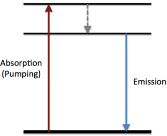
Optical fibers can amplify light at correct wavelength through stimulated emis-sion. This is done by optically pumping the gain fiber to obtain population inversion. [20] For Ytterbium gain fibers we have used, lasing scheme is classified as a three-level scheme as shown in Figure 1.3. [21, 22] Ytterbium ions absorb pump photons to reach an excited state then relax rapidly into a lower-energy excited state. The life time of this intermediate state is usually long (around 1ms for Ytterbium), and the stored energy is used to amplify incident light (also called seed signal) through stimulated emission. The dopant finally ends up in the ground state.

(13)

Figure 1.2: Schematic of a fiber amplifier

with a moderate power levels. The gain efficiency can be very high. [23] An important limiting factor to the gain is the generation of Amplified Spontaneous Emission (ASE), that is the self amplification of spontaneously emitted photons. To reach higher powers, moderate gain stages are usually used to suppress ASE generation and be power-wise more efficient.

The amplifiers are usually saturated to get the most out of the amplifier. This allows higher output powers, resulting with less excess pumped ions. Excessively pumped gain leads to ASE generation. [16] ASE also provides the fundamental limitation of the amplifier noise properties.

1.2 Modeling of Amplifiers

Modelling of these amplifiers are possible with rate equations where the popula-tion levels of excited and ground states as well as the pump and signal powers are calculated. [24]

(14)

Figure 1.3: Three level system

Optical pumping creates the necessary population inversion between two en-ergy states and provides the optical gain. The rate equations for calculating the upper and lower state population levels n1(z, t) and n2(z, t) are:

dn1(z, t) dt = p,a Pp(z, t) Ah⌫p + s,a Ps(z, t) Ah⌫s ! n1(z, t) + p,e Pp(z, t) Ah⌫p + s,e Ps(z, t) Ah⌫s + ⌧ ! n2(z, t) (1.3) dn2(z, t) dt = p,a Pp(z, t) Ah⌫p + s,a Ps(z, t) Ah⌫s ! n1(z, t) p,e Pp(z, t) Ah⌫p + s,e Ps(z, t) Ah⌫s + ⌧ ! n2(z, t) (1.4)

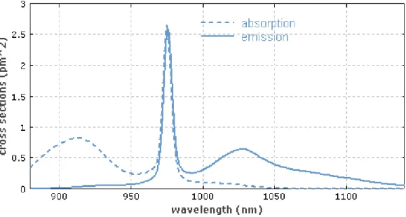
where a and e are the e↵ective absorption and emission cross sections.

Fig-ure 1.4 shows example cross section curves for Yb doped fibers. Pp and Ps denote

the pump and signal power levels. ⌫p and ⌫s are the pump and signal frequencies,

respectively. ⌧ is the gain relaxation time (upper state lifetime), A is the core area and z is the propagation axis.

The change in power levels are defined as: dPp(z, t)

dt = p[ p,an2(z, t) p,en1(z, t)] Pp(z, t) (1.5) dPs(z, t)

dt = s[ s,an2(z, t) s,en1(z, t)] Ps(z, t) (1.6)

(15)

Figure 1.4: Absorption and emission cross section curves for Yb+ _ions.

fiber region.

Eq.’s (1.3), (1.4), (1.5) and (1.6) can be numerically solved using the Runge-Kutta method. [25]

1.3 Relative Intensity Noise of Laser Signals

The output of a mode-locked fiber laser is repeating high energy pulses where the repetition rate is determined by the laser cavity roundtrip. These repeating pulses are represented by equally distant Dirac-deltas functions In the frequency domain. When this signal is transferred to an electrical signal at a photodetector, the DC component will be detected as well.

The intensity noise, that is the coincidental fluctuations of the laser signal intensity in time, is best measured in the frequency domain by analysing the contributions of di↵erent frequency components. (Figure 1.5) The DC component (also called baseband) is preferred as it is easier to measure. [26]

(16)

Figure 1.5: Diagram of RIN measurement

measurement of DC will depend on the average intensity of the laser signal. The obtained baseband spectra can be divided by the voltage level to obtain the relative noise spectra, that is the Relative Intensity Noise (RIN).

The total rms RIN (also called integrated RIN) can be calculated by integrat-ing the RIN up to Nyquist frequency. This is no boundintegrat-ing limit as the typical spectra for mode locked fiber lasers show low noise profile at high frequencies (200 kHz).

(17)

Chapter 2 Characterisation of Relative

Intensity Noise of Fibre

Amplifiers

We utilise two di↵erent amplifiers, a core-pumped, low-power (output <1 W) am-plifier with a single-mode diode laser as pump and a cladding-pumped, high-power (output up to 50 W) amplifier with multiple multi-mode diode lasers as pump. In the latter case, additional intermediate amplifier stages are present between the amplifier under characterisation and the seed oscillator. The measurement and characterisation setup is common for both cases.

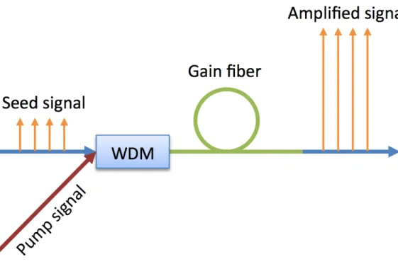
We employ the core-pumped, low-power amplifier as in Figure 2.1 due to its ease of experimentation. The amplifier comprises of 120 cm long Yb-doped fibre with 278 dB/m absorption at 976 nm. The amplifier is forward pumped through a wavelength division multiplexer (WDM) by a single-mode pump diode operating at a central wavelength of 976 nm. The fibre has a core diameter of 7 µm, core numerical aperture of 0.08 and cladding diameter of 250 µm. A portion of the output of the pump diode and that of the amplifier output are directed to the power meter or the baseband analyser where the RIN is measured. The amplified signal is separated from any unabsorbed pump signal.

(18)

Figure 2.1: Single-clad fiber amplifier setup

The double-clad amplifier consists of a multi-pump combiner (MPC) with 5 pump ports, connected to a low-doped double-clad Yb-fibre, followed by a high-doped Yb fibre. (Figure 2.2) The low-high-doped segment is 1.8 m long with 6.5 dB/m absorption at 980 nm, and the high-doped segment is 1.6 m long with 10.8 dB/m absorption at 980 nm. Both fibres have a core diameter of 25 µm, core numerical aperture of 0.08, cladding diameter of 250 µm, which enables very low-loss splicing between them. We employ two 25-W diodes and three 32-W diode, all operating at 976 nm, for pumping the gain.

Due to the di↵erent emission cross-section values of Yb+ _{ions along its span}

range, we have characterised the amplifier noise at two di↵erent seed signal wave-lengths. These seed signals are provided from a similariton [27] fibre laser at 1030 nm and an all normal dispersion fibre laser at 1060 nm centre wavelengths both with 20 nm bandwidth. The laser outputs are split by a fibre coupler, where one port is directed to a high-resolution power meter or a low-noise baseband analyser (R&S UPV) for analysis and the other port seeds the amplifier.

(19)

Figure 2.2: Double-clad fiber amplifier setup

2.1 Relative Intensity Noise of Pump, Seed and

Amplified Signals

2.1.1 Relative Intensity Noise of Pump Signal

The laser diode modules used to pump the gain at 976 nm are semiconductor continuos wave lasers with fibre coupled outputs. The laser used for low power operation is attached to a fibre with 5 um core diameter, that is low enough to support single-mode operation only. The fibre also incorporates fibre bragg gratings, that transmit the light at a certain wavelength and reflect at other wavelengths back into the cavity, consequently to stabilise the wavelength. This increases the quality factor of the laser and the stability as well.

The pump lasers used for high power operation are attached to fibres with 105 um core diameter. This fibre has an advantage of allowing higher powers as more light can propagate. The waveguide supports multiple modes of light.

(20)

0 50k

100k

150k

200k

250k

10

13

10

12 2· 10 14 2_{· 10} 12

⌫ (Hz)

RIN

(

1 /

Hz

)

Figure 2.3: Experimentally obtained RIN curves of pump, seed, ASE and ampli-fied signals for single-clad amplifier

2.1.2 Relative Intensity Noise of Seed Signal

The similariton laser, that is used as a seed source, works on the basis of self similar propagating pulses, that is basically an asymptotic solution to the nonlin-ear Schrodinger equation. The all normal dispersion laser, that is the other seed source, works on having normal dispersion along every point of the laser cavity and having a filter to shorten the dispersed pulses by cutting the edges of the pulse both in time and spectral domains. This filter is centred at 1060 nm to force the laser to work at 1060 nm. The pulse duration is 5 ps.

The noise of the seed signal is given in Figure 2.3 (red-dotted) and Figure 2.4 (red-dotted). The projected low noise level is ideal for use as seed source, since the noise will be amplified as well. These lasers show relatively low noise levels as compared to other mode-locked fibre lasers.

(21)

2.1.3 Relative Intensity Noise of Amplified Spontaneous

Emission

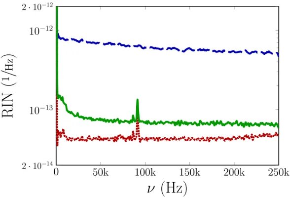
The random nature of spontaneous emission exhibits noise. When spontaneously emitted photons are amplified instead of a regular seed signal in an amplifier, the output becomes more noisy. Experimentally, ASE can be easily obtained by pumping the gain but blocking the seed signal. The output will be propagating in both directions of the fibre. The noise measurement of this signal is shown in Figure 2.3 (blue-dashed). The noise level corresponds to a level that is higher than of the pump and seed signals at least by an order of magnitude.

2.1.4 Relative Intensity Noise of Amplified Signal

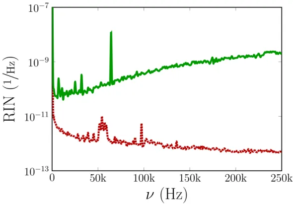
Typical noise profile for a single cladding Yb-doped fibre amplifier is shown in Figure 2.3 (green-solid) for seed and pump powers of 12 mW and 100 mW, re-spectively. The integrated (from 1 kHz to 250 kHz) RIN values for the single-clad amplifier output are measured and calculated to be 0.0192%± 0.0005 and 0.0190%± 0.0005, respectively. Figure 2.4 (green-solid) shows the RIN of double-clad amplifier output at 1.5 W of seed and 72 W pump powers. The integrated RIN values are measured to be 1.42%_{± 0.05 and 2.00% ± 0.05, respectively.}

To realise the low noise working regimes, we characterize the RIN of fiber-amplified pulses as a function of both seed and pump powers. (Figure 2.5) The general behavior is as to be expected: the combination of low seed and high pump powers leads to excessive ASE generation, which increases the RIN level. The integrated RIN is observed to decreases rapidly with increasing seed under con-stant pump power. We note that for the similar experiment with seed wavelength of 1060 nm, 4 times higher seed power is required compared to seeding at 1030 nm. Stronger seed is required to saturate the amplifier at 1060 nm, compared to 1030 nm, leading to less ASE generation, due to the lower transition cross section of the Yb-doped fiber at the former wavelength.

(22)

0 50k

100k

150k

200k

250k

10

13

10

11

10

9

10

7

⌫ (Hz)

RIN

(

1 /

Hz

)

Figure 2.4: Experimentally obtained RIN curves of pump, seed and amplified signals for double-clad amplifier

of the core signal but the noise as well. The higher the excess pump signal, the higher the ASE generation will be. This mapping provides intuition on how much noisy the signal will be and suggests to simulate the gain equations in order to get an estimation of ASE generation.

2.2 Reduction of Multimode Pump Laser Noise

Enroute to Low Noise High Power

Ampli-fiers

In high power fibre systems, large amount of pump signal is needed. The multi pump combiners are used to combine pump signals coming from multiple number of laser diodes. The output power as well as the noise of each laser signal will add on top of each other in the temporal domain.

(23)

4

8 ₁₆

₃₂

₆₄

128

256

512

400

350

300

250

200

150

100

50 P

s

(0) (

µW)

P

p

(0

)

(mW)

0.02%

0.03%

0.04%

0.05%

0.06%

Figure 2.5: Contour graphs of integrated RIN of amplified signal for seed signal center wavelengths of (a) 1030 nm and (b) 1060 nm for varying pump and seed powers

A significant contribution of noise in the double clad amplifiers come from multi-mode pump diodes. The di↵erent modes in the waveguide propagate at di↵erent velocities. Due to the inhomogeneities in the fibre, such as in refractive index and geometry, the modes exchange energy and this causes randomness exposed on the power levels, that is uncorrelated between each laser signal. [28, 29]

However the dominating part of the noise is imparted by the coupling from the electrical source, that pumps the laser diode itself. The noise of the electrical source is transferred to the laser signal. For practical reasons, a single electrical source is preferred to drive the large number of laser diodes. However this imposes correlated noise on each laser signal.

We demonstrate the averaging of intensity noise over multiple pump diodes with incoherent noise profile. For this experiment, each laser diode is supplied by di↵erent electrical source. The noise of combination of multimode diodes is characterised at the output of an MPC with 8 input ports as described in Figure

(24)

Figure 2.6: Combination of multiple multi-mode pump diodes setup 2.6. The 25 W diodes are turned on or o↵ accordingly.

The RIN of the combination of diodes is observed to decrease with inverse square root of number of diodes combined. (Figure ;combinations (gray dots) and mean values (black dots)) The squares in the figure correspond to measurements on a setup with possible correlated noise sources. The results show that using a combination of multiple diodes supplied from di↵erent sources running at low power instead of a single diode running at high power results in a lower noise profile.

(25)

0

1

2

3

4

5

6

7

8

9

0.02

0.04

0.06

0.08

0.1

0.12 Number of diodes

In

tegr

at

ed

RIN

(%

)

Figure 2.7: Integrated RIN values for combinations of multiple multi-mode pump diodes

(26)

Chapter 3 Modulation Transfer Functions

To investigate the coupling of noise from pump and seed signals to the ampli-fied signal, we follow a well known approach of modulating the source and then measuring the modulation at the output, just like a network analyser. The ra-tio of output to input gives out modulara-tion transfer rara-tio as described in Eq.’s (3.1) and (3.2). We scan this for a range of modulation frequencies and obtain the modulation transfer function (MTF). [30] We measure these functions exper-imentally and confirm theoretically by numerical solving of time injected laser rate equations.

M odulation T ransf er Ratiopump signal =

Output M odulationamplif ied signal

Input M odulationpump signal

(3.1) M odulation T ransf er Ratioseed signal =

Output M odulationamplif ied signal

Input M odulationseed signal

(3.2)

3.1 Measurement of Modulation Transfer

Func-tions

The MTFs are measured by modulating the pump and seed powers and measuring the modulation at the output of the amplifier.

(27)

Figure 3.1: MTF Measurement Setup

acousto-optic modulator (AOM) to modulate the seed signal (Figure 3.1). The AOM works on the basis of acousto-optics e↵ect by di↵racting the beam using a voltage driven piezoelectric crystal. [31, 32] The seed signal traverses through the AOM and is modulated by the driving frequency.

The pump signal can be modulated using the modulation input of its driver. The diode driver has a modulation transfer function of its own, which is not disturbing our measurement as long as modulation can be transferred and there is no resonant frequency within our modulation range. The waveform generator is connected to the diode driver to transfer modulation over the frequency range of 1 Hz - 250 kHz, where the upper limit is set by the bandwidth of the audio analyser. However, the entire measurement is automated via a computer using LabVIEW (Figure B.1).

(28)

3.2 Calculation of Modulation Transfer

Func-tions

We decouple the fast and slow dynamics governing the amplification of broadband pulses in a fiber amplifier as follows: The fast dynamics is modeled by a general-ized nonlinear Schr¨odinger equation as in [33], using an e↵ective gain model. The gain parameters are determined from a more accurate model based on laser rate equations, where the signal power is interpreted as the average power of the pulse train. This is justified as long as the repetition rate is in the MHz range or higher and no individual pulse is energetic enough to saturate the amplifier. The model is then valid for both continuous wave and pulsed signal amplification. We use a generalised version of this well-known model to include modulations (as well as noise) of the seed and the pump. [34, 35, 36] The signal and pump modulations and population levels at a specific frequency of ! = 2⇡⌫ are described by:

Pp(s)(z, t) = P1(2),0(z)(1 + q1(2)(z, !)ei!t) + c.c. (3.3)

n1(2)(z, t) = n3(4),0(z)(1 + q3(4)(z, !)ei!t) + c.c., (3.4)

where Pp(s)(z, t) are the pump (signal) intensities and n1(2)(z, t) are the

frac-tional population densities of the lower (upper) states, and q(z, !) represent the modulation amplitudes; c.c. denotes complex conjugate. Pp(s),0(z) and n1(2),0(z)

correspond to solutions without modulation that is described in Chapter 1.2. z denotes position along the gain fiber of total length L.

We would like to solve the rate equations for the power modulation amplitudes, namely q1(z, !) and q2(z, !). We have already described the rate equations in

Chapter 1.2 as: dn1(z, t) dt = p,a Pp(z, t) Ah⌫p + s,a Ps(z, t) Ah⌫s ! n1(z, t) + p,e Pp(z, t) Ah⌫p + s,e Ps(z, t) Ah⌫s + ⌧ ! n2(z, t) (3.5) dn2(z, t) dt = p,a Pp(z, t) Ah⌫p + s,a Ps(z, t) Ah⌫s ! n1(z, t)

(29)

p,e Pp(z, t) Ah⌫p + s,e Ps(z, t) Ah⌫s + ⌧ ! n2(z, t) (3.6)

We insert Eq.’s (3.3) and (3.4) into Eq.’s (3.5) and (3.6) to first order to find: 0 = p,aPp(z) Ah⌫p n1(z) p,ePp(z) Ah⌫p n2(z) ! q1(z, !) + s,aPs(z) Ah⌫s n1(z) s,e Ps(z) Ah⌫s n2(z) ! q2(z, !) + p,aPp(z) Ah⌫p + s,aPs(z) Ah⌫s ! n1(z)q3(z, !) p,ePp(z) Ah⌫p + s,ePs(z) Ah⌫s + ⌧ iw ! n2(z)q4(z, !) (3.7) 0 = p,aPp(z) Ah⌫p n1(z) p,e Pp(z) Ah⌫p n2(z) ! q1(z, !) s,aPs(z) Ah⌫s n1(z) s,e Ps(z) Ah⌫s n2(z) ! q2(z, !) p,aPp(z) Ah⌫p + s,aPs(z) Ah⌫s iw ! n1(z)q3(z, !) + p,ePp(z) Ah⌫p + s,ePs(z) Ah⌫s + ⌧ ! n2(z)q4(z, !) (3.8)

We may rewrite Eq.’s (3.7) and (3.8) as:

f (z)q1(z) + g(z)q2(z) + h(z)q3(z) [gg(z) iwn2(z)] q4(z) = 0 (3.9) f (z)q1(z) g(z)q2(z) [h(z) iwn1(z)] q3(z) + gg(z)q4(z) = 0 (3.10) where we define: f (z) = p,aPp(z) Ah⌫p n1(z) p,e Pp(z) Ah⌫p n2(z) g(z) = s,aPs(z) Ah⌫s n1(z) s,e Ps(z) Ah⌫s n2(z) h(z) = p,aPp(z) Ah⌫p + s,aPs(z) Ah⌫s ! n1(z) gg(z) = p,ePp(z) Ah⌫p + s,ePs(z) Ah⌫s + ⌧ ! n2(z)

(30)

We have defined the power equations in Chapter 1.2 as: dPp(z, t)

dt = p[ p,an2(z, t) p,en1(z, t)] Pp(z, t) (3.11) dPs(z, t)

dt = s[ s,an2(z, t) s,en1(z, t)] Ps(z, t) (3.12)

By inserting Eq.’s (3.3) and (3.4) into Eq.’s (3.11) and (3.12) we find:

" p( p,an2(z) p,en1(z))Pp(z) dPp(z) dz # q1(z) Pp(z) dq1(z) dz p p,en1(z)Pp(z)q3(z) p p,an2(z)Pp(z)q4(z) = 0 (3.13) " s( s,an2(z) s,en1(z))Ps(z) dPs(z) dz # q2(z) Ps(z) dq2(z) dz s s,en1(z)Ps(z)q3(z) s s,an2(z)Ps(z)q4(z) = 0 (3.14)

We may rewrite Eq. (3.13) and Eq. (3.14) as: k(z)q1(z) Pp(z) dq1(z) dz m(z)q3(z) + r(z)q4(z) = 0 (3.15) l(z)q2(z) Ps(z) dq2(z) dz q(z)q3(z) + s(z)q4(z) = 0 (3.16) where we define k(z) = p( p,an2(z) p,en1(z))Pp(z) dPp(z) dz m(z) = p p,en1(z)Pp(z) r(z) = p p,an2(z)Pp(z) l(z) = s( s,an2(z) s,en1(z))Ps(z) dPs(z) dz q(z) = s s,en1(z)Ps(z) s(z) = s s,an2(z)Ps(z)

Using Eq.’s (3.9) and (3.10) we form 2 constraint equations for q3(z) and q4(z).

By adding Eq.’s (3.9) and (3.10) we obtain: q4(z)

q3(z)

= n1(z) n2(z)

(31)

By subtracting Eq. (3.10) from Eq. (3.9) we obtain: q3(z) = 2 u(z)[f (z)q1(z) + g(z)q2(z)] (3.18) where u(z) = 2h(z) + 2n1(z) n2(z) g(z) + 2iwn1(z) (3.19)

Inserting Eq.’s (3.17) and (3.18) into Eq.’s (3.15) and (3.16) for q3(z) and

q4(z) gives: k(z)q1(z) Pp(z) dq1(z) dz + m(z) + r(z)n1(z) n2(z) ! 2 u(z)[f (z)q1(z) + g(z)q2(z)] = 0 (3.20) l(z)q2(z) Ps(z) dq2(z) dz + q(z) + s(z)n1(z) n2(z) ! 2 u(z)[f (z)q1(z) + g(z)q2(z)] = 0 (3.21)

Grouping for q1(z) and q2(z) in Eq.’s (3.20) and (3.21) we obtain:

X(z)q1(z) Pp(z) dq1(z) dz + Y (z)q2(z) = 0 (3.22) XX(z)q2(z) Ps(z) dq2(z) dz + Y Y (z)q1(z) = 0 (3.23) where X(z) = k(z) + 2 u(z)f (z) " m(z) + r(z)n1(z) n2(z) # = 0 Y (z) = 2 u(z)f (z) " m(z) + r(z)n1(z) n2(z) # = 0 XX(z) = l(z) + 2 u(z)g(z) " q(z) + s(z)n1(z) n2(z) # = 0 Y Y (z) = 2 u(z)g(z) " q(z) + s(z)n1(z) n2(z) # = 0

Eq.’s (3.22) and (3.23) along with Eq.’s (3.11) and (3.12) are numerically solved for q1(z), q2(z), Pp(z) and Ps(z) with the Runge-Kutta method with

(32)

The initial modulation is set by assigning modulation amplitudes to q1(z = 0)

and q1(z = 0) in the simulation parameters for either seed or pump signals. The

initial seed and pump powers are set by Ps(z = 0) and Pp(z = 0). q1(z = 1.2)

and q2(z = 1.2) give the modulation amplitudes at the end of the fiber. The

simulations are repeated for modulation frequency w, from 1 Hz to 250 kHz. Each simulation takes around 1 second to calculate the modulation transfer ratio.

The modulation transfer functions (MTF), ⇠p(⌫) for pump and ⇠s(⌫) for signal

are defined as:

⇠p(⌫) = q2(L, ⌫) q1(0, ⌫) (3.24) ⇠s(⌫) = q2(L, ⌫) q2(0, ⌫) (3.25) which are essentially Lorentzian-like in shape, as will be discussed. An in-herent assumption is that the modulation amplitudes are small enough that the dynamics is linear.

3.3 Characterisation of Modulation Transfer

Functions

The experimental results are compared with results obtained from the calculations for Yb-fiber amplifiers, which are pumped through the core and the cladding, where the physics of noise transfer is identical, but strong technical di↵erences exist due to the use of single-mode and multi-mode pump sources, respectively.

Measured (dots) and calculated (curve) MTF’s for the case of 1 mW of seed and 100 mW of pump power are illustrated in Figure 3.2. These MTF’s can be fit very well by generalised Lorentzian functions, which will provide parameters for these functions and thus a workaround.

The generalised MTF’s are given by: ⇠p(⌫) = ⇠p,0

"

1 + ⌫

⌫p,0

(33)

1

10

100 1k

10k

100k

0

0.5

1

1.5

⌫ (Hz)

⇠

p

,

⇠

s

Figure 3.2: Typical MTF curves for the pump and

⇠s(⌫) = 1

1 ⇠s,0

1 +⇣ ⌫ ⌫s,0

⌘n

for the seed.

In these functions, ⇠p,0 and ⇠s,0 represent the small frequency transfer

coef-ficients, that we call the plateau values as well. ⌫p and ⌫s are the 3-dB cuto↵

frequencies for pump and signal, respectively.

A prerequisite for using the transfer function approach is that the system under study must be linear. Indeed, the small-frequency transfer coefficients, ⇠p,0

and ⇠s,0, are verified to be independent of the modulation depth over a large range

of modulation depths as shown in Figure 3.3.

⇠p,0 and ⇠s,0, and the 3-dB cuto↵ frequencies, ⌫p,0 and ⌫s,0over the ratio of the

(34)

10

0

6

10

5

10

4

10

3

10

2

10

1

0.5

1

1.5 Relative Modulation

⇠

p,

0 ,

⇠

s,

0

Figure 3.3: MTF parameter for varying input modulation amplitudes transfer coefficients for pump and seed always approach 0 and 1, respectively, at high frequencies, meaning that high-frequency pump noise has practically no in-fluence on amplifier performance. Conversely, any seed modulations are strongly suppressed at low frequencies due to the saturation e↵ect. By saturating the am-plifier, the e↵ect of slight variations of pump power on the signal output power can be substantially reduced. As the signal and pump MTF’s are complementary, rendering possible broadband modulation (e.g., for CEP stabilisation) by modu-lating both the seed and the pump at high and low frequencies, respectively.

(35)

100 4 ₁₀ 2 ₁₀0 ₁₀2 0.5 1 1.5 Ps(0)

/

_P_p₍₀₎

⇠

p,0

,

⇠

s,0 10 3 ₁₀ 2 ₁₀ 1 ₁₀0 0 8k 16k 24k 32k Ps(0)

/

_P_p₍₀₎

⌫

p, 0

,

⌫

s, 0

(Hz)

(36)

Chapter 4 Prediction of Noise of Fibre

Amplifiers

As an application, we utilise the theoretical model to predict amplifier intensity noise using the leading noise sources, which are the RIN present on the seed signal, the contribution of the pump laser noise and excess quantum noise due to amplified spontaneous emission (ASE). Nominally, a full calculation of combined e↵ect of these noise processes is extremely demanding in terms of computation time, as an integration time of at most half of the inverse of the lowest frequency of interest is required, that is the Nyquist rate. [37] Most of the pump- and environment-induced noise appears at low frequencies (typically, few kHz or less). Given that the largest integration step can be the cavity round trip time for a pulsed laser (typically 10-20 ns), a full-fledged simulation of the noise dynamics requires up to 108 _{steps for a single calculation and many more iterations might}

be required if some statistical information is desired.

Our approach, however, is based on using the MTF of signal and pump to determine the average RIN to be imparted at each frequency on the amplifier output based on the RIN value of the signal and the pump at that frequency.

Thus, we treat noise due to signal or pump and amplified spontaneous emission to be additive in nature. This approach promptly ignores any interaction between

(37)

0 50k

100k

150k

200k

250k

10

13

10

12 2· 10 14 2_{· 10} 12

⌫ (Hz)

RIN

(

1 /

Hz

)

Figure 4.1: Predicted RIN curves of pump, seed, ASE and amplified signals for single-clad amplifier

these noise sources and assumes linear contribution. The independency of MTFs on modulation amplitude suggests us a hint on linear coupling of noise.

We inherently assume that all noise sources introduce weak enough fluctua-tions that they can be treated as first-order perturbafluctua-tions. The average relative intensity noise of the amplifier output is given by,

RINamp(⌫) = ⌘1[RINs(⌫)⇠s(⌫) + RINp(⌫)⇠p(⌫)]

+⌘2[RINase(⌫) + RINp(⌫)⇠a(⌫)] (4.1)

Here, ⌘1 and ⌘2 represent the fractional power of coherent (amplified signal)

and incoherent (ASE) portions of the amplifier output, respectively. ⇠a(⌫) is

the pump-to-ASE MTF, which has the same form as ⇠p(⌫) with correspondingly

di↵erent parameters. We note that ⇠p(⌫) is exactly a Lorentzian. RINs(⌫) and

(38)

0 50k

100k

150k

200k

250k

10

13

10

11

10

9

10

7

⌫ (Hz)

RIN

(

1 /

Hz

)

Figure 4.2: Predicted RIN curves of pump, seed, ASE and amplified signals for double-clad amplifier

The amplified spontaneous emission constitutes white noise given by

RINase(⌫) = ⌫opt1, (4.2)

where ⌫opt is the optical bandwidth of the ASE spectrum [38].

The pump and seed RIN contributions, weighted by their respective transfer functions, and RIN due to ASE are all added up linearly, which ignores any interaction between these noise sources. This is justified as long as the noise levels are low.

Figure 4.1 shows the measured RIN of the seed (red-densely dotted), ASE (blue-dashed), amplifier output (green-solid) and calculated RIN of ASE (gray-dot dashed) and amplifier output (black-loosely (gray-dotted) for seed and pump powers of 12 mW and 100 mW, respectively. Calculated RIN for strong seed and ASE reveal very good agreement with the experimental results. The integrated (from 1 kHz to 250 kHz) RIN values for the single-clad amplifier output are measured and

(39)

4µ

₁₆

µ

₆₄

µ

256 µ

1m

_12m

0.01

0.03

0.05

0.07 P

s

(0) (W)

In

tegr

at

ed

RIN

(%

)

(a)

0 ₁₀

₂₀

₃₀

₄₀

₅₀

0

1

2

3 P

s

(L) (W)

In

tegr

at

ed

RIN

(%

)

(b)

Figure 4.3: Crosssection of Integrated RIN

calculated to be 0.0192%± 0.0005 and 0.0190% ± 0.0005, respectively. Figure 4.2 shows the RIN of measured seed (red-dotted) and double-clad amplifier output (green-solid) and calculated amplifier output (black-solid) at 1.5 W of seed and 72 W pump powers. The integrated RIN values are measured and calculated to be 1.42%_{± 0.05 and 2.00% ± 0.05, respectively.}

Figure 4.3 (a) shows the cross-section of Figure 2.5 for pump power of 400 mW and corresponding predicted RIN values. The integrated RIN is observed to decrease rapidly with increasing seed under constant pump power. Figure 4.3 (b) is the predicted integrated RIN for DC amplifier for varying output powers at constant seed power. The integrated RIN is observed to stay constant over the output power range of 5 W to 50 W with seed power of 1.5 W.

(40)

Chapter 5 Fibre interferometer based

low-noise vibrometer

Highly sensitive displacement measurement is one of the main goals in many fields ranging from astronomy, metrology to gravitational wave detection. [39] Here we show the use of a fiber interferometer in detecting kHz regime vibrations with precision up to 4 nm. The setup is based on a modified Michelson Interferometer. (Figure 5.1) [40] A low noise continuous wave laser signal that is at 1.5 um centre wavelength, passes through a coupler. The coupler splits the incoming signal to 50% at each output. One end of the coupler is dumped. The other end is cleaved and used as the probe in directing the light and detecting vibrations. The cleaved fibre will reflect some portion of the light that comes from the coupler and the rest will go out. From the outgoing light, some portion will be reflected back from the vibrating sample and will couple back into the fibre. A microscope is built below the sample to align the fiber tip with the sample. The two reflected lights, from the fibre tip and the sample, go though the coupler and interference is observed at the detector. The intensities at the detector will be:

Idetector = If ibretip+ Isample+ 2

q

If ibretipIsamplecos (5.1)

where If ibretipand Isample are the intensities of light reflected from the fiber tip

(41)

Figure 5.1: Fiber interferometer setup

The intensities If ibretip and Isample highly depend on the reflection coefficients.

The detected intensity at the detector can be rewritten in terms of the intensity of the initial beam I0 as:

Idetector = I0 2 h Rf ibretip+ Rsample+ 2 q

Rf ibretipRsamplecos

i

(5.2)

where Rf ibretip and Rsample are the reflection coefficients of the fiber tip and

the sample.

The sinusoidal part in Eq. (5.2) results in interference fringes. The phase di↵erence is related to the distance z between the fiber tip and the sample as shown in Figure 5.1. can be written in terms of z as:

= 2⇡2d (5.3)

The interference fringes from an axial scan is shown in Figure 5.2. Maximizing the reflection coefficients will increase the amplitude of the interference fringes and thus the signal to noise ratio. The unwanted environmental vibrations and the noise of the laser signal are the dominant noise contributors. As well as a fiber interferometer being a flexible setup, another advantage is the common path

(42)

0 2 4 6 8 10 12 14 0 0.005 0.01 0.015 0.02 0.025 0.03

z (um)

Detector Voltage (V)

Figure 5.2: Interference fringes observed at the detector

noise cancellation as both signals travel through the same fiber. This makes the system relatively resistant to environmental vibrations.

To test the ability of detecting vibrations, a piezo actuator has been placed below the fiber. Measured vibrations of 4 nm amplitude at 1 kHz is illustrated in Figure 5.4 in time and frequency domains. The noise floor of the measurement shows relatively higher noise at frequencies up to around 200 Hz. This shows difficulty in measuring steady distances and slow vibrations. However at higher frequencies, the measurement becomes much more accurate with higher signal to noise ratio and sub-5 nm vibrations up to 380 kHz can be detected, frequency limited by the sampling rate of out measurement device.

(43)

0 5 10 15 20 25 30 0.0523 0.0524 0.0525 0.0526 0.0527 Time (ms) Detector Voltage (V) 101 102 103 104 0 1 2 3 4x 10 −4 Frequency (Hz) Detector Voltage (V)

Figure 5.3: Observation of 4 nm amplitude kHz regime vibrations in the time and frequency domain measurements

5.1 Vibrational Spectroscopy

The experimental setup in Figure 5.1 can be modified to use as a vibrational spectrometer. A piezo translation stage is integrated to hold and intentionally vibrate a sample on a petri dish. Similar to the MTF measurements in practice, the vibrational response of a living cell or a micro particle can be measured. Our motivation is to build a device that can determine the vibrational resonance frequencies of di↵erent cells with regards to their shape and inner structure, and to be able to distinguish between unknown cells, such as cancerous cells.

(44)

Figure 5.4: Diagram of Vibrational spectroscopy experiment

and not present below the fiber. The ratio of these two measurements will give out the normalized vibrational response of the sample. The response can be shown as:

N ormalized V ibrational Response = M easured V ibrationwith sample M easured V ibrationwithout sample

(5.4)

This measurement is scanned from 1 Hz to 250 kHz to realize a vibrational spectroscopy of the sample. This curve will be flat if the response of the cell is linear, and nonlinear when the sample is in mechanical resonance with the oscillating piezo stage.

We plan on using this technique to detect the vibrations of neurons, as a way to realize the presence of an action potential. The vibration of a neuron during action potential is an assumption based on the piezo-electric property of the cell membrane. [41] Progress has been made with crab nerve cells and crayfish axon. [42, 43] However these measurement setups are not robust and higher resolutions are needed. The current setup is capable of 4 nm resolution and there is ongoing work to determine the resonance frequency of H9C2 cells.

(45)

Chapter 6 Conclusion

In summary, we have characterized the noise and transfer of seed and pump mod-ulations to the output of a fiber amplifier and confirmed this with an analytical model. The obtained results are used as a practical application to predict the intensity noise of an amplifier, obtaining excellent agreement with experiments. In the future, we plan to apply the modulation transfer approach to a laser os-cillator, which is expected to lead to qualitatively di↵erent results due to the feedback provided by the cavity. We have shown that using a combination of multiple diodes running at low power instead of a single diode running at high power results in a lower noise profile. Experimental development of low-noise fiber laser amplifiers can be guided by theory with high accuracy.

We have developed a low noise vibrometer that is capable of detecting sub-5 nm kHz regime vibrations. This device is planned to be used in detecting neuronal activity as a very robust and easy to use replacement to traditional cumbersome electrophysiology experiment setups.

(46)

Bibliography

[1] N. A. Olsson, “Lightwave systems with optical amplifiers,” Journal of Light-wave Technologies, vol. 7, p. 1071, 1989.

[2] D. O. Caplan, “Laser communication transmitter and receiver design,” Jour-nal of Optical Fiber Communications, vol. 4, p. 225, 2007.

[3] G. P. Agrawal, “Fiber-optic communication systems,” John Wiley and Sons, 2002.

[4] H. J. R. Dutton, “Understanding optical communications,” IBM Redbooks, 2002.

[5] W. ONeill and K. Li, “High-quality micromachining of silicon at 1064 nm using a high-brightness mopa-based 20-w yb ber laser,” IEEE Journal of Selected Topics in Quantum Electronics, vol. 15, pp. 462–470, 2009.

[6] M. Erdogan, B. Oktem, H. Kalaycioglu, S. Yavas, P. Mukhopadhyay, K. Eken, K. Ozgoren, Y. Aykac, U. H. Tazebay, and F. O. Ilday, “Textur-ing of titanium (ti6ai4v) medical implant surfaces with mhz-repetition-rate femtosecond and picosecond yb-doped ber lasers,” Optics Express, vol. 19, p. 10986, 2011.

[7] M. Murakami, B. Liu, Z. Hu, Z. Liu, Y. Uehara, and Y. Che, “Burst-mode femtosecond pulsed laser deposition for control of thin lm morphology and material ablation,” Applied Physics, vol. 2, p. 042501, 2009.

[8] P. K. Mukhopadhyay, K. Ozgoren, I. L. Budunoglu, and F. O. Ilday, “All-fiber low-noise high-power femtosecond yb-“All-fiber amplifier system seeded by

(47)

an all-normal dispersion fiber oscillator,” IEEE Journal of Selected Topics in Quantum Electronics, vol. 15, pp. 145 – 152, 2009.

[9] I. L. Budunoglu, C. Ulgudur, B. Oktem, and F. O. Ilday, “Intensity noise of mode-locked fiber lasers,” Optics Letters, vol. 34, pp. 2516 – 2518, 2009. [10] N. R. Newbury and W. C. Swann, “Low-noise fiber-laser frequency combs

(invited),” Journal of Optical Society of America B, vol. 24, pp. 1756 – 1770, 2007.

[11] S. B. Poole, D. N. Payne, and M. E. Fermann, “Fabrication of low loss optical fibers containing rare earth ions,” Electronics Letters, vol. 21, p. 737, 1985. [12] S. B. Poole, “Fabrication and characterization of low-loss optical fibers

con-taining rare earth ions,” Journal of Lightwave Technologies, vol. 7, p. 870, 1986.

[13] K. C. Kao and G. A. Hockham, “Dielectric-fiber surface waveguides for op-tical frequencies,” Proceedings of IEEE, vol. 113, p. 1151, 1966.

[14] K. C. Kao and T. W. Davies, “Spectrophotometric studies of ultra low loss optical glasses i: Single beam method,” Journal of Physics E, vol. 2, p. 1063, 1968.

[15] A. W. Snyder and J. D. Love, “Optical waveguide theory,” Chapman and Hall, 1983.

[16] G. P. Agrawal, “Nonlinear fiber optics,” Elsevier, 2007.

[17] Kouznetsov and J. V. Moloney, “Efficiency of pump absorption in double-clad fiber amplifiers. ii. broken circular symmetry,” Journal of Optical Society of America B, vol. 19, p. 1259, 2001.

[18] V. Filippov, “Double clad tapered fiber for high power applications,” Optics Express, vol. 16, p. 1929, 2008.

[19] D. J. Ripin, “High efficiency side-coupling of light into optical fibres using embedded v-grooves,” Electronics Letters, vol. 31, p. 2204, 1995.

(48)

[20] C. J. Koester and E. Snitzer, “Amplification in a fiber laser,” Applied Optics, vol. 10, p. 1182, 1964.

[21] M. Obro, “Highly improved fibre amplifier for operation around 1300 nm,” Electronics Letters, vol. 27, p. 470, 1991.

[22] R. Paschotta, “Ytterbium-doped fiber amplifiers,” IEEE Journal of Elec-tronics, vol. 33, p. 1049, 1997.

[23] J. Limpert, “High-power femtosecond yb-doped fiber amplifier,” Optics Ex-press, vol. 14, p. 628, 2002.

[24] C. R. Giles and E. Desurvire, “Modeling erbium-doped fiber amplifiers,” Journal of Lightwave Technology, vol. 9, p. 271, 1991.

[25] J. C. Butcher, “Numerical methods for ordinary di↵erential equations,” John Wiley and Sons, 2003.

[26] R. Scott and C. L. B. Kolner, “High-dynamic-range laser amplitude and phase noise measurement techniques,” IEEE Journal of Selected Topics in Quantum Electronics, vol. 7, p. 641, 2001.

[27] F. O. Ilday, J. Buckley, and F. W. Wise, “Self-similar evolution of parabolic pulses in a laser cavity,” Physical Review Letters, vol. 92, pp. 2139021 – 2139024, 2004.

[28] A. W. Snyder, “Coupled-mode theory for optical fibers,” Journal of Optical Society of America, vol. 11, p. 1267, 1972.

[29] A. V. Smith and J. J. Smith, “Mode instability in high power fiber ampli-fiers,” Optics Express, vol. 19, p. 10180, 2011.

[30] T. D. Mulder, R. P. Scott, and B. H. Kolner, “Amplitude and envelope phase noise of a modelocked laser predicted from its noise transfer function and the pump noise power spectrum,” Optics Express, vol. 16, pp. 14186–14191, 2008.

(49)

[31] R. Lucas and P. Biquard, “Optical properties of solid and liquid medias subjected to high-frequency elastic vibrations,” Journal of Physics, vol. 71, pp. 464 – 477, 1932.

[32] C. B. Scruby and L. E. Drain, “Laser ultrasonics: Techniques and applica-tions,” Taylor and Francis, 1990.

[33] B. Oktem, C. Ulgudur, and F. O. Ilday, “Solition-similariton fibre laser,” Physical Review Letters, vol. 4, pp. 307 – 311, 2010.

[34] S. Novak and A. Moesle, “Analytic model for gain modulation in edfas,” Journal of Lightwave Technology, vol. 20, pp. 975–985, 2002.

[35] J. Freeman and J. Conradi, “Gain modulation response of erbium-doped fiber amplifiers,” IEEE Photonics Technology Letters, vol. 5, pp. 224–226, 1993.

[36] M. Trobs, P. Wessels, and C. Fallnich, “Power- and frequency-noise char-acteristics of an yb-doped fiber amplifier and actuators for stabilization,” Optics Express, vol. 13, pp. 2224–2235, 2005.

[37] Y. Geerts, M. Steyaert, and W. Sansen, “Design of multi-bit delta-sigma a/d converters,” Springer, 2002.

[38] H. Hodara, “Statistics of thermal and laser radiation,” Proceedings of the IEEE, vol. 53, pp. 696 – 704, 1965.

[39] P. Hariharan, “Basics of interferometry,” Elsevier, 2007.

[40] J.-B. Decombe, W. Schwartz, C. Villard, H. Guillou, J. Chevrier, S. Huant, and J. Fick, “Living cell imaging by far-field fibered interference scanning optical microscopy,” Optics Express, vol. 19, pp. 2702 – 2710, 2011.

[41] K. Iwasa, I. Tasaki, and R. C. Gibbons, “The capacitance and electrome-chanical coupling of lipid membranes close to transitions: The e↵ect of elec-trostriction,” Biophysical Journal, vol. 103, pp. 918–929, 2012.

[42] T. Heimburg, “Swelling of nerve fibers associated with action potentials,” Science, vol. 210, pp. 338–339, 1980.

(50)

[43] B. C. Hill, E. D. Schubert, M. A. Nokes, and R. P. Michelson, “Laser in-terferometer measurement of changes in crayfish axon diameter concurrent with action potential,” Science, vol. 196, p. 426, 1977.

(51)

Appendix A

Data

Example Simulation Parameters:

Parameter Matlab Variable Value Unit

Modulation frequency mod frequency 100 Hz

Initial pump power Pp0 100x10 3 _W

Initial seed power Ps0 1x10 3 _W

Gain fibre length L 1.2 m

Pump center wavelength NUp 976x10 9 _m

Seed center wavelength NUs 1030x10 9 _m

Pump absorption cross section SIGMAap 2.74x10 24 _m2

Pump emission cross section SIGMAep 2.74x10 24 _m2

Seed absorption cross section SIGMAas 5.97x10 26 _m2

Seed emission cross section SIGMAes 6.8x10 25 _m2

Ion concentration in the gain fibre N 3.1x1025 _{ions per m}3

Upper state lifetime TAU 0.85 ms

Seed overlap factor GAMMAs 0.73xN

Pump overlap factor GAMMAp 0.764xN

Fibre core radius a 1.5x10 6 _m

(52)

Appendix B

Code

Contents of mtr.m

1 function out=mtr(mod frequency,Pp0,Ps0,Qp0,Qs0)

2 format long;

3 %% VARIABLES

4 global W L NUp NUs SIGMAap SIGMAep SIGMAas SIGMAes GAMMAp GAMMAs ...

N H TAU a A 5 L=1.2; 6 W=2*pi*mod frequency; 7 NUp=(3*10ˆ8)/(976*10ˆ( 9)); 8 NUs=(3*10ˆ8)/(1030*10ˆ( 9)); 9 SIGMAap=2.74*10ˆ( 24); 10 SIGMAep=2.74*10ˆ( 24); 11 SIGMAas=5.97*10ˆ( 26); 12 SIGMAes=6.8*10ˆ( 25); 13 N=3.1*10ˆ25; 14 GAMMAp=0.764*N; 15 GAMMAs=0.73*N; 16 H=6.6256*10ˆ( 34); 17 TAU=1*10ˆ( 3); 18 a=1.5*10ˆ( 6); 19 A=pi*aˆ2; 20

(53)

21 %% CALCULATIONS 22 out1=ode45(@odes,[0 L],[Qp0 0 Qs0 0 Pp0 Ps0]); 23 out=sqrt(out1.y(3,length(out1.y))ˆ2... 24 +out1.y(4,length(out1.y))ˆ2)/(Qp0+Qs0); 25 26 %% SUBFUNCTIONS 27 28 function result=odes(z,Q) 29 P1=Q(5); 30 P2=Q(6);

31 global GAMMAp GAMMAs SIGMAep SIGMAes SIGMAap SIGMAas

32 result=[... 33 1/P1*( Xi(z,P1,P2)*Q(2)+Xr(z,P1,P2)*Q(1)... 34 Yi(z,P1,P2)*Q(4)+Yr(z,P1,P2)*Q(3));... 35 1/P1*(Xi(z,P1,P2)*Q(1)+Xr(z,P1,P2)*Q(2)... 36 +Yi(z,P1,P2)*Q(3)+Yr(z,P1,P2)*Q(4));... 37 1/P2*( XXi(z,P1,P2)*Q(4)+XXr(z,P1,P2)*Q(3)... 38 YYi(z,P1,P2)*Q(2)+YYr(z,P1,P2)*Q(1));... 39 1/P2*(XXi(z,P1,P2)*Q(3)+XXr(z,P1,P2)*Q(4)... 40 +YYi(z,P1,P2)*Q(1)+YYr(z,P1,P2)*Q(2));... 41 GAMMAp*(SIGMAep*N2(z,P1,P2) SIGMAap*N1(z,P1,P2))*P1;... 42 GAMMAs*(SIGMAes*N2(z,P1,P2) SIGMAas*N1(z,P1,P2))*P2... 43 ]; 44 45 function result = f(z,P1,P2)

46 global NUp SIGMAap SIGMAep H A

47 result=N1(z,P1,P2)*(P1*SIGMAap)/(A*H*NUp)...

48 N2(z,P1,P2)*(P1*SIGMAep)/(A*H*NUp);

49

50 function result = g(z,P1,P2)

51 global NUs SIGMAas SIGMAes H A

52 result=N1(z,P1,P2)*(P2*SIGMAas)/(A*H*NUs)...

53 N2(z,P1,P2)*(P2*SIGMAes)/(A*H*NUs);

54

55 function result = gg(z,P1,P2)

56 global NUs SIGMAep SIGMAes H A TAU NUp

57 result=((P1*SIGMAep)/(A*H*NUp)+(P2*SIGMAes)...

58 /(A*H*NUs))*N2(z,P1,P2)+(1/TAU)*N2(z,P1,P2);

59

(54)

61 global NUs SIGMAap SIGMAas H A NUp

62 result=((P1*SIGMAap)/(A*H*NUp)+(P2*SIGMAas)...

63 /(A*H*NUs))*N1(z,P1,P2);

64

65 function result = m(z,P1,P2)

66 global SIGMAap GAMMAp

67 result=GAMMAp*SIGMAap*N1(z,P1,P2)*P1;

68

69 function result = q(z,P1,P2)

70 global SIGMAas GAMMAs

71 result=GAMMAs*SIGMAas*N1(z,P1,P2)*P2;

72

73 function result = r(z,P1,P2)

74 global SIGMAep GAMMAp

75 result=GAMMAp*SIGMAep*N2(z,P1,P2)*P1;

76

77 function result = s(z,P1,P2)

78 global SIGMAes GAMMAs

79 result=GAMMAs*SIGMAes*N2(z,P1,P2)*P2;

80

81 function result = realinvu(z,P1,P2)

82 global W

83 result=(2*hh(z,P1,P2)+2*N1(z,P1,P2)/N2(z,P1,P2)...

84 *gg(z,P1,P2))/((2*hh(z,P1,P2)+2*N1(z,P1,P2)/N2(z,P1,P2)...

85 *gg(z,P1,P2))ˆ2+(2*W*N1(z,P1,P2))ˆ2);

86

87 function result = imageinvu(z,P1,P2)

88 global W 89 result= (2*W*N1(z,P1,P2))/((2*hh(z,P1,P2)+2*N1(z,P1,P2)... 90 /N2(z,P1,P2)*gg(z,P1,P2))ˆ2+(2*W*N1(z,P1,P2))ˆ2); 91 92 function result = Xr(z,P1,P2) 93 result=2*(f(z,P1,P2)*m(z,P1,P2)+N1(z,P1,P2)... 94 /N2(z,P1,P2)*r(z,P1,P2)*f(z,P1,P2))*realinvu(z,P1,P2); 95

96 function result = Xi(z,P1,P2)

97 result=2*(f(z,P1,P2)*m(z,P1,P2)+N1(z,P1,P2)...

98 /N2(z,P1,P2)*r(z,P1,P2)*f(z,P1,P2))*imageinvu(z,P1,P2);

99

(55)

101 result=2*(g(z,P1,P2)*m(z,P1,P2)+N1(z,P1,P2)...

102 /N2(z,P1,P2)*r(z,P1,P2)*g(z,P1,P2))*realinvu(z,P1,P2);

103

104 function result = Yi(z,P1,P2)

105 result=2*(g(z,P1,P2)*m(z,P1,P2)+N1(z,P1,P2)... 106 /N2(z,P1,P2)*r(z,P1,P2)*g(z,P1,P2))*imageinvu(z,P1,P2); 107 108 function result = XXr(z,P1,P2) 109 result=2*(q(z,P1,P2)*g(z,P1,P2)+N1(z,P1,P2)... 110 /N2(z,P1,P2)*s(z,P1,P2)*g(z,P1,P2))*realinvu(z,P1,P2); 111

112 function result = YYr(z,P1,P2)

113 result=2*(q(z,P1,P2)*f(z,P1,P2)+N1(z,P1,P2)...

114 /N2(z,P1,P2)*s(z,P1,P2)*f(z,P1,P2))*realinvu(z,P1,P2);

115

116 function result = XXi(z,P1,P2)

117 result=2*(q(z,P1,P2)*g(z,P1,P2)+N1(z,P1,P2)...

118 /N2(z,P1,P2)*s(z,P1,P2)*g(z,P1,P2))*imageinvu(z,P1,P2);

119

120 function result = YYi(z,P1,P2)

121 result=2*(q(z,P1,P2)*f(z,P1,P2)+N1(z,P1,P2)...

122 /N2(z,P1,P2)*s(z,P1,P2)*f(z,P1,P2))*imageinvu(z,P1,P2);

123

124 function result = N2(z,P1,P2)

125 global NUp NUs SIGMAap SIGMAep SIGMAas SIGMAes GAMMAp GAMMAs...

126 H TAU A N 127 result=((P1*GAMMAp*SIGMAap)/(N*A*H*NUp)+(P2*GAMMAs*SIGMAas)... 128 /(N*A*H*NUs))/((P1*GAMMAp*(SIGMAap+SIGMAep))/(N*A*H*NUp)... 129 +(P2*GAMMAs*(SIGMAas+SIGMAes))/(N*A*H*NUs)+1/TAU); 130 131 function result = N1(z,P1,P2) 132 result=1 N2(z,P1,P2); 133

134 function result=rk4(a, b, N, initial)

135 h = (b a)/N; 136 z(1) = a; 137 q(:,1) = initial; 138 for i = 1:N 139 q1 = h*odes(z(i), q(:,i)); 140 q2 = h*odes(z(i)+h/2, q(:,i)+0.5*q1);

(56)

141 q3 = h*odes(z(i)+h/2, q(:,i)+0.5*q2); 142 q4 = h*odes(z(i)+h, q(:,i)+q3); 143 q(:,i+1) = q(:,i) + (q1 + 2*q2 + 2*q3 + q4)/6; 144 z(i+1) = a + i*h; 145 end 146 result=[z' q']; Contents of lorentzian.m 1 function [y]=lorentzian(variables,v) 2 ksi0=variables(1); 3 ksi1=variables(2); 4 v0=variables(3); 5 n=variables(4); 6 y=ksi1+ksi0./(1+(v./v0).ˆn); Contents of lorentzian2.m 1 function [y]=lorentzian(variables,v) 2 ksi0=variables(1); 3 v0=variables(2); 4 n=variables(3); 5 y=ksi0./(1+(v./v0).ˆn); Contents of mtf.m 1 function out=mtf(Pp0,Ps0,Qp0,Qs0) 2 tic 3 frequency=2.ˆ(1:0.5:18.5); 4 out1=zeros(1,length(frequency)); 5 frequencyfit=2.ˆ(2:0.1:25.5); 6 for f=1:ceil(length(frequency)/4) 7 spmd 8 format long; 9 out1(4*(f 1)+labindex)=sum(mtr(frequency(4*(f 1)... 10 +labindex),Pp0,Ps0,Qp0,Qs0)); 11 end

(57)

12 end

13 out2=(out1{1}+out1{2}+out1{3}+out1{4});

14 [constants]=nlinfit(frequency,out2,@lorentzian,[0.5,0,5e3,1.5]);

15 %[constants]=nlinfit(frequency,out2,@lorentzian2,[0.5,5e3,1.5]);

16 disp(['ksi0=' num2str(constants(1)+constants(2))])

17 % disp(['ksi0=' num2str(constants(1))])

18 disp(['ksi1=' num2str(constants(2))])

19 disp(['v0=' num2str(constants(3))]) 20 disp(['n=' num2str(constants(4))]) 21 % disp(['ksi0=' num2str(constants(1))]) 22 % disp(['v0=' num2str(constants(2))]) 23 % disp(['n=' num2str(constants(3))]) 24 semilogx(frequency,out2,'.',frequencyfit... 25 ,lorentzian(constants,frequencyfit)) 26 beep;pause(0.2);beep;pause(0.2);beep 27 toc 28 out=[frequency' out2'];

(58)

Figure B.1: LabVIEW Automated MTF and Vibrational Spectrescopy measure-ment design