Effects of Reordering and Lumping in the
Analysis of Discrete-Time SANs
TUGRUL DAYAR1 Department of Computer Engineering, Bilkent University, 06533 Bilkent, Ankara, Turkey. tugrul<Ocs. bilkent. edu. tr
Abstract. In a recent paper [13J, it is shown that discrete-time stochastic automata net-works (SANs) are lumpable under rather general conditions. Therein, the authors present an efficient iterative aggregation-disaggregation (lAD) algorithm geared towards comput-ing the stationary vector of discrete-time SANs that satisfy the conditions of lumpability. The performance of the proposed lAD solver essentially depends on two parameters. The first is the order in which the automata are lined up, and the second is the size of the lumped matrix. Based on the characteristics of the SAN model at hand, the user may have some flexibility in the choice of these two parameters. In this paper, we give rules of thumb regarding the choice of these parameters on a model from mobile communications. Key words. Stochastic automata networks, discrete-time Markov chains, lumpability, iterative aggregation-disaggregation
1 Introd uction
Stochastic Automata Networks (SANs) [19, 20, 22, 21, 23, 11, 25, 12, 26, 6, 2, 4, 9, 27, 28, 3, 10, 13) comprise a methodology for modeling Markovian systems that have interacting components. The methodology is based on decomposing the system to be investigated into its components and modeling each component in-dependently. Afterwards, interactions and dependencies among components are introduced and the model finalized. The two advantages of SANs that result from this divide-and-conquer approach are the following. Each component can be mod-eled much easier compared to the global system due to state space reduction. Storage space allocated for components is minimal compared to the case in which transitions from each global state are stored explicitly. However, all this comes at the expense of longer analysis time [12, 26, 2, 6, 4, 9, 27, 3, 13).
A discrete-time system of N components can be modeled by a single stochas-tic automaton for each component. With this decompositional approach, the global system ends up having as many states as the product of the number of states of the individual components. See [25, Ch. 9) for detailed information regarding SANs. When there are E synchronizing events in the system, automaton k denoted by A(k) has the corresponding transition probability matrix Pe(k) that represents the contribution of A(k) to synchronization e E {O, 1, ... , E - I} (see [10, p. 333)). For convenience, we number the automata and synchronizing events starting from
o.
The underlying discrete-time MC (DTMC) corresponding to the global system can be obtained fromE-1 N-1
P=
L
®p~k). (1)e=O k=O
IThis work is supported by TUBiTAK-CNRS grant.
210 Mathematics and Computer Science
We refer to the tensor representation in equation (I) associated with the DTMC as the descriptor of the SAN. Assuming that A(k) has nk states, the global system has n
=
rrf=~l nk states. When there are transition probabilities in p~k) that are functions of the global state of the system rather than only A(k), tensor products become generalized tensor products [23]. We consider the form of the descriptor in equation (I) rather than the one in [19] since it is compact and easier to work with.The difficulty associated with discrete-time SANs is that the matrices p~k)
are relatively dense compared to their continuous-time counterparts implying a larger number of floating-point arithmetic operations in the generalized descriptor-vector multiply algorithm (see [9, p. 404]) used in iterative solvers. Generally, the underlying DTMC of a discrete-time SAN is a dense matrix as opposed to the generator corresponding to a continuous-time SAN. Therefore, discrete-time SANs can be used to tackle even small systems composed of interacting components but that have dense DTMCs since the underlying MC is not generated and stored during SAN analysis.
In the next section, we provide information about the wireless ATM model that is investigated. In the third section, we discuss the results in [13] related to ordering and lumping of automata. In the fourth section, we provide results of numerical experiments, and in the fifth section, we conclude.
2 The model
The application considered in [13] is a multiservices resource allocation policy (MRAP) that integrates three types of service over a time division multiple access (TDMA) system in a mobile communication environment. We have the constant bit rate (CBR) service for two types of voice calls (i.e., handover calls from neigh-boring cells and new calls), the variable bit rate (VBR) service for two types of calls as in CBR service, and the available bit rate (ABR) service for data transfer. A single cell and a single carrier frequency is considered, and the system is modeled as a discrete-time SAN in which state changes occur at TDMA frame boundaries. Regarding the events that take place in the system, the following assumptions are made. Data packet and call arrivals to the system happen at the beginning of a frame, and data packet transmissions finish and calls terminate at the end of the frame. Since each data packet is small enough to be transmitted in a single slot of a TDMA frame, in a particular state of the system it is not possible to see slots occupied by data packets.
Now, let us move to the parameters of the model. Data is queued in a FIFO buffer of size B and has the least priority. The arrival of data packets is modeled as an on-off process. The process moves from the on state to the off state with probability a and vice versa with probability {3. The load offered to the system is defined as A = {3/ {a
+
{3). Assuming that the time interval between two con-secutive on periods is t, the burstiness of such an on-off process is described by the square coefficient of variation,Se
=
Var{t)/[E{t}F. In terms of A and Se,on state, we assume that i E
{O,
1,2, 3} data packets may arrive with probability Pdi. The mean arrival rate of data packets is defined as p=
I:~=1 iX
Pdi. Hence, the global mean arrival rate of data packets is given byr
= Ap. If the number of arriving data packets exceeds the free space in the buffer plus the number of free slots in the current TDMA frame, the excess packets are dropped.Handover CBR requests have priority over new CBR calls and they respec-tively arrive with probabilities Ph and Pn. Similarly, the probabilities of VBR new call and handover arrivals during a TDMA frame have geometrical distributions with parameters Pvn and Pvh, respectively. We do not consider multiple handover or new CBR/VBR call arrivals during a TDMA frame since the associated prob-abilities with these events are small. Each CBR/VBR call takes up a single slot of a TDMA frame but may span multiple TDMA frames. When all the slots are full, incoming CBR/VBR calls are rejected. The number of CBR calls that may terminate in a TDMA frame depends on the number of active CBR calls, but can be at most M, and hence is modeled as a truncated binomial process with parameter Ps.
On the other hand, a VBR connection is characterized by a state of high intensity and a state of low intensity. In the former, the VBR source transmits data with its peak rate, whereas in the latter, its transmission rate is lower. The reduced transmission rate in the low intensity state in fact means that at some instances of time the slot in a TDMA frame allocated to the VBR connection is not used. A VBR connection moves from the high intensity state to the low intensity state with probability O:v and vice versa with probability f3v· In terms of Av = f3v/(O:v
+ f3v)
and its square coefficient of variation Se v' we have f3v
=
2Av (1-Av) / (Be v+
1-Av) and O:v=
f3v (1 - Av) / Av. When in the low intensity state, the VBR connectionmoves from the case of a busy slot to the case of an empty slot with probability Pempty and vice versa with probability Pbusy. State changes of a VBR connection after it is set up are assumed to take place at the end of a TDMA frame. We further assume that when a VBR connection is set up as either a new call or a handover, it is in the high intensity state. However, the connection can terminate in any state of the VBR source. We also assume that when a VBR connection changes its state from high intensity to low intensity, it enters the state with a busy slot. The number of VBR calls that may terminate in a TDMA frame depends on the number of active VBR calls and the duration of each VBR call is assumed to be a geometric process with parameter Pvs.
Each TDMA frame that gives CBR, VBR, and ABR service consists of
C
slots reserved for CBR traffic and V slots reserved for VBR traffic. ABR traffic can be pushed into any reserved, but unused slots. Hence, data packets can be trans-mitted in the idle slots among the C reserved for CBR traffic, in the idle slots among the V reserved for VBR traffic, and in those slots among the V that are in the low intensity state but are empty. The SAN model consists of (3+ V) automata and 9 synchronizing events. States of all automata are numbered starting from O.We denote the state index of automaton k by sA(k). Automaton A(O) represents the data arrival process and has two states that correspond to the on and off states of the data source. Transitions in this automaton happen independently of other automata. Automaton A(1) represents the portion of the TDMA frame reserved
212 Mathematics and Computer Science
for CBR calls and has (C
+
1) states. Automaton A (2) represents the data buffer and has (B + 1) states, where B is the buffer size. Transitions of this automata depend on A(O) and A(1). Automata A(3) through A(2+V) represent the V slots reserved for VBR traffic. Each automaton corresponding to VBR traffic has four states. State 0 of the automaton corresponds to the case of an idle slot, i.e., the VBR connection is not active. State 1 corresponds to the state of high intensity state, states 2 and 3 correspond to the state of low intensity. Particularly, state 2 indicates that the slot is busy and state 3 indicates that it is empty. Each automa-ton A(k), k E {4, 5, ... , V+
2}, that models VBR traffic depends on the automata A(3) ,A(4), ... , A(k-I) since we assume that arriving VBR calls are dispatched to slots starting from the smallest indexed VBR automaton. We remark that the au-tomata of the SAN that handle CBR and VBR arrivals are mutually independent. Hence, the set of synchronizing events are given by Cartesian product, and eab denotes the synchronizing event that is triggered by a CBR arrivals and b VBR arrivals for a, bE {O, 1, 2}.The probability matrices associated with the automata are all relatively dense except the ones that correspond to the data buffer when
sA
(0)=
O.
See[13]
for a detailed description of the system. In passing, we remark that the discrete-time SAN model of the system has a global state space size of n=
2(C+
1)(B + 1)4v. For the problem with (C, V, B) = (8,2,15), A = 0.1, Se=
1, (PdO,Pdl,Pd2,Pd3)=
(0.05,0.1,0.25,0.6) (amounting to an average of p = 2.5 packet arrivals during a TDMA frame), (Pn,Ph,Ps) = C(5 X 10-6,10-5,5 x 10⁻⁶ ), Av = 0.5, Sev = 10, (Pempty,Pbusy) = (0.9,0.1), (Pvn,Pvh,Pvs) = V(5 x 10-6,10-5,5 x 10⁻⁶ ), and atmost 2(= M) CBR departures during a TDMA frame, we have n = 4,608 and
nz = 1,618,620 (number of nonzeros larger than 10-16 is 1,174,657). Here nz
denotes the number of nonzeros in the underlying DTMC.
We refer to the rejection of an existing call as dropping and to the rejection of a new call or packet as blocking. The performance measures of interest are the dropping probabilities of handover CBR and handover
vnR
calls, the blocking probabilities of new CBR calls and new VBR calls, and the blocking probability of data packets. Once the steady state vector of the descriptor is computed, each of the performance measures may be determined[13].
[n this work, the aim is not to present values of performance measures for a set of parameters, but rather is to discuss the implications on the lAD solver of reordering the automata and choosing the size of the lumped matrix. Therefore, we constrain ourselves to re-porting solution times and iteration counts in section 4. Now, let us summarize the theoretical results in[13].
3 Reordering and Lumping
The automata of some discrete-time SANs can be reordered and then renumbered so that transitions of A (k) for k E {I, 2, ... , N -I} depend (if at all) on the states of the lower indexed automata A(O), A(1), ... , A(k-l) (the functional dependency be-ing represented by A(k) [A(O) , A(1), ... ,A(k-I)]) (see
[9]
for details). Note that there must exist at least one automaton (in our case, it isA
(0)) that is independent of allthe other automata for such an ordering to be possible. In our model, such an or-dering of automata is possible, and it implies that the automaton
A
(2) be placed in the last position and the automata A(k), k E {3, 4, ... , V +2}, be placed in any po-sition other than the last as long as they are ordered according to increasing index among themselves. Hence, one possibility is A (0), A (1), A (3), A (4), ... ,A (V +2), A (2). Now, let us assume that the automata are reordered as described and renum-bered from°
to (N - 1). To such an ordering of automata correspond block par-titionings of the form(2)
in which all the blocks Pij are square, of order n~=-~ nk, and K
=
n;;=~l nk for any m E {I, 2, ... , N - I}. Hence, for the given ordering of automata, there are (N - 1) different such partitionings which vary between one that has no diagonal blocks of order n~=-;.l nk and one that has n~=~2 nk diagonal blocks of order nN-l' Each of the (N - 1) block partitionings is lump able as stated in the next theorem of [13].Theorem 1 A discrete-time SAN of N automata and E synchronizing events whose automata are reordered and renumbered so that A(k) [A(O) , A(l), ... , A(k-l)J, k E {I, ... , N - I}, and that has the descriptor in equation (1) with equal row sums in each p~k) for k
=
0, 1, ... , N - 1 and e=
0,1, ... , E - 1 is lumpable with respect to the partitioning in equation (2) for any mE {1, 2, ... , N - 1}.Now, we state the more relaxed version of Theorem 1 in [13] for the case of cyclic functional dependencies.
Definition 1 Let G(V, [) be the directed graph (digraph) corresponding to a discrete-time SAN in which the vertex Vk E V represents A(k) and the edge (Vk' vt}
E E if transitions in A(k) depend on the state of A(l) (i.e., A(k) [A(l)]). Then the SAN is said to contain cyclic functional dependencies if and only if the digraph has at least one strongly connected component (SeC) composed of multiple automata. Detailed description of the
see
algorithm for digraphs can be found in [1, pp. 191-197].Theorem 2 A discrete-time SAN of N automata A(k), k
=
0,1, ... , N - 1, and E synchronizing events that contains cyclic functional dependencies among its automata is lumpable if the digraph corresponding to the SAN has more than onesec
and each p~k) has equal row sums for k = 0,1, ... , N - 1 and e = 0,1, ... ,E-1.
Assuming that P is lumpable with respect to the partition in (2) and is irreducible, in [13] the following modified form of Koury-McAllister-Stewart's lAD
214 Mathematics and Computer Science
algorithm [15] is proposed for computing the stationary probability vector 7r (i.e.,
7rP = 7r, 117r11 = 1). The convergence analysis of the KMS algorithm is based on the concept of near complete decomposability (NCD) [18]. In [16] and [24], it is shown that fast convergence is achieved if the degree of coupling, 11F11oo, is small compared to 1, where P
=
F+diag(Pll,P22 , ... ,PKK).Algorithm 1. lAD algorithm for discrete-time SANs
1. Let 7r(O) = (7riO) , 7r~O) , ... , 7r~») be a given initial approximation of 7r. Set it
=
1.2. Aggregation:
(a) Compute the lumped matrix L of order K with ijth element
lij
=
max(Piju).(b) Solve the singular system 7(I - L) = 0 subject to 1171h = 1 for
7
=
(71, 72, ... , 7K).3. Disaggregation:
(a) Compute the row vector
(b) Solve the K nons in gular systems of which the ith is given by
(it)(l _ p .. ) _ b(it)
7ri U - i
for 7rjit) , i
=
1,2, ... ,K, whereb(it) _ ' " (it)p .. i - ~ Zj Jt
+ '"
~ 7rj (it)p .. Jt· j>i j<i4. Test 7r(it) for convergence. If the desired accuracy is attained, then stop and take 7r(it) as the stationary probability vector of P. Else set it = it
+
1 and go to step 3.In [17], the convergence of a framework of lAD methods is studied. The lAD algorithm considered is different in that there is no requirement of NCDness on the partitioning. Furthermore, a number of relaxations (i.e., smoothings) of the power method kind is performed at the fine level. The authors prove that the errors at the fine and coarse levels are intimately related, and for a strictly positive initial approximation, the lAD approximation converges rapidly to the stationary vector as long as one is very precise in computing at the coarse level and a sufficiently high number of smoothings is performed at the fine level. Numerical results on randomly generated stochastic matrices with varying degrees of coupling and having equal
orders of blocks which are all tridiagonal show that convergence is practically independent of the degree of coupling.
The motivation behind proposing Algorithm 1 rather than block Gauss-Seidel (BGS) for discrete-time SANs is that the partitioning in (2) is a balanced one with equal orders of blocks and the aggregate matrix needs to be formed only once due to lumpability. See [8] for recent results on the computation of the stationary vector of Markov chains.
In Algorithm 1, the lumped matrix L of order K
=
nZ'=~1 nk is computed at the outset and solved once for its stationary vector T. Note that the lumped matrix L is also lumpable if m>
1. These hint at the solver to be chosen at step 2 to compute T. Assuming that L is dense, one may opt for a direct solversuch as Gaussian elimination (G E) (or the method of Grassmann-Taksar-Heyman, GTH, if L is relatively ill-conditioned) when K is on the order of hundreds. Else one may use lAD with a lumped matrix of order
nZ'~~l
nk, where 1<
m'<
m(or lAD with an NCD partitioning if L is relatively ill-conditioned). In any case, sufficient space must be allocated to store L. As for the disaggregation phase (i.e., a BGS iteration), the right-hand sides b~it) at iteration it may be computed efficiently as shown in [13] at the cost of E(K - 2) vectors of length
n:=-':'
nk, that is roughly E vectors of length n. In summary, the proposed solver is limited by max(K2 , (E + 2)n) amount of double precision storage assuming that the lumped matrix is stored in two dimensions. The 2 vectors of length n are used to store the previous and current approximations of the solution.So far, we have assumed that the underlying DTMC of the given discrete-time SAN is irreducible. Since this may not be the case, a state classification (SC) algorithm that partitions the global state space of a SAN into essential and tran-sient subsets is implemented [13]. The inhibition of trantran-sient states is important in removing redundant computation from the lAD solver. However, the case of more than one partition of essential states is not considered since it hints at a modeling problem.
Now, let us return to the model in section 2 and consider lumpable orderings of the automata. Since A (2) must be the last automaton in a lumpable order-ing, there are (V
+
I)! ways in which A(D) may precede A(l) among the first(V
+
2) automata. The same argument is true of A(D) succeeding A(l) among the first (V+
2) automata. Therefore, the requirement in Theorem 1 regarding functional dependencies implies that there are 2(V + I)! orderings that may be used. Hence, we have 12 lumpable orderings to choose from when V = 2 and 48 lumpable orderings to choose from when V=
3. Since these are large num-bers of orderings to investigate, we treat the VBR automata as a single entity and concentrate on only the 3! orderings of automata given by [(3,4, ... , V+
2),1,0,2]' [1,(3,4, ... ,V+
2),0,2]' [(3,4, ... ,V+
2),0,1,2]' [0,(3,4, ... ,V+
2),1,2]' [1,0, (3,4, ... , V+
2),2]' and [0,1, (3,4, ... , V+
2),2]. We name these orderings respectively 01,02, ... ,06' Regarding the lumping parameter, m, we choose valuesfrom the set {V -1, V, V
+
I} which implies that the largest lumped matrix formed in step 2 is of order 2(C+
1)4v and the smallest system to solve in step 3 is of order (B + 1).216 Mathematics and Computer Science
We remark that a reordering of discrete-time automata corresponds to a symmetric permutation of the underlying DTMC. In other words, reordering of automata is equivalent to a renumbering of the global states in a SAN model. Since the objective of this study is to investigate the effects of reordering and the lumping parameter, m, on the convergence of Algorithm 1, we choose the integer parameters (C, V, B) so that the lumped matrix formed in step 2 can be solved accurately and rapidly using the GTH method as discussed in [7] and there is sufficient space to factorize in sparse format the K diagonal blocks in step 3(b) at
the outset. Hence, we use sparse forward and back substitutions to solve the K
nonsingular systems at each iteration of Algorithm 1 and do not need to employ any smoothings.
4
Numerical results
Algorithm 1 is implemented in C++ as part of the software package PEPS [22]. We time the solver on a Pentium III with 64 MBytes of RAM under Linux. In each experiment, we use a tolerance of 10-8 on the approximate error 117r(it) - 7r(it-1) 112
in step 4 of Algorithm 1. The approximate residual 117r(it) - 7r(it) Pl12 turns out to
be less than the approximate error upon termination in all our experiments. In the first set of experiments, we consider three variants of the problem
(C, V, B) = (8,2,15), which has a state space size of n = 4,608 (see section 2). We set (PdO,Pd1,Pd2,Pd3) = (0.05,0.1,0.25,0.6), Av = 0.5, SCv = 10, (Pempty,Pbusy) =
(0.9,0.1) in the first variant and (PdO,Pd1,Pd2,Pd3) = (0.4,0.3,0.2,0.1), Av = 0.5,
SCv = 1, (Pempty,Pbusy) E {(O.g, 0.1), (0.5, 0.5)} in the last two variants. The other parameters are chosen as M = V, Sc = 1, A E {0.1, 0.3, 0.5, 0.7, 0.9}, (Pn,Ph,Ps) =
C(5 X 10-6,10-5,5 x 10⁻⁶), and (Pvn,Pvh,Pvs) = V(5 X 10-6,10-5,5 x 10⁻⁶). The lump ability parameter assumes the values in {2, 3, 4}. The degree of coupling,
11F11oo, associated with the partitioning in equation (2) for each DTMC is on
the order of 10-1 and mostly close to 1.0. Hence, the lumpable partitionings we consider in Algorithm 1 for the first set of experiments are not NCD. However, the smallest degree of coupling we find for each DTMC using the algorithm in [5] is on the order of 10-5 . All this means that even though the lumpable partitionings we consider are not NCD partitionings, there exist highly NCD partitionings for each DTMC, and therefore they are all very ill-conditioned.
The underlying DTMCs of the SAN models in the first set of experiments are reducible with a single subset of essential states and 224 transient states. It
is argued in [13] that when a reducible discrete-time SAN has a single subset of essential states and each subset of the partition in equation (2) includes at least one essential state (which is the case in our experiments), the lumped matrix com-puted in step 2 of Algorithm 1 is irreducible. With such a partitioning, if one starts in step 1 with an initial approximation having zero elements corresponding to transient states, successive computed approximations will have zero elements corresponding to transient states as well. In our experiments, we start with a positive initial approximation and observe that all elements that correspond to transient states become zero at the second iteration. Once the elements that
cor-respond to transient states in an approximate solution become zero, they remain zero. Hence, there is no need to run the time consuming SC algorithm for each of the experiments, since the matrices in each of the three variants have the same nonzero structure.
In the first variant, Algorithm 1 converges for the orderings 01 and 02 within
34 iterations when m E {3, 4}, whereas for the other four orderings it converges within 34 iterations only when m = 4. In all other cases, Algorithm 1 does not converge within 250 iterations to the prespecified tolerance. A similar observation follows for the second and third variants if we replace the 34 respectively with 65 and 120 (achieved in 04-06). Hence, the three variants of this problem seem to be of
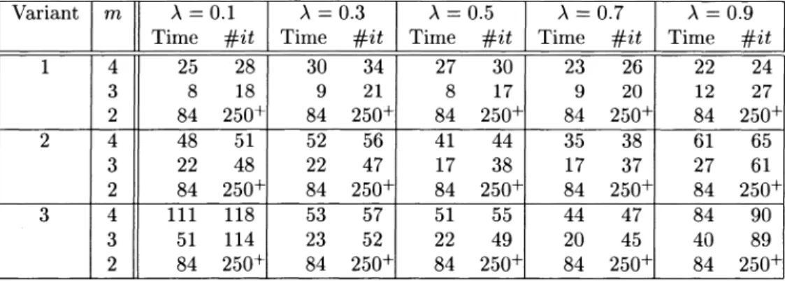
increasing difficulty as we move from the first to the third, although each one has highly NCD partitionings with degree of coupling on the same order of 10-5 . In Table 1, we present the results of numerical experiments with Algorithm 1 for the three variants using 01. Note that a smaller number of iterations may not imply
a smaller solution time as in the first variant for A = 0.9. The best solution times are obtained with 01 (and 02) when m
=
3 is used. For each of the six orderings, m=
4 gives a lumped matrix of order K=
288. For 01 and 02, m=
3 gives a lumped matrix of order K = 144. For the other four orderings, m = 3 gives lumped matrices of orders 32 and 72, which are both smaller than 144. For the six orderings, m = 2 gives lumped matrices of orders varying between 8 and 36. Ittakes nearly 0 seconds to solve the lumped matrix using GTH in all cases. Hence, the timing results in Table 1 are for the iterative part of Algorithm 1.
TABLE 1. Solution times in seconds and
#
of iterations with 01 for 1st set of experiments.Variant m A
=
0.1 A=
0.3 A=
0.5 A=
0.7 A=
0.9 Time #it Time #it Time #it Time #it Time #it1 4 25 28 30 34 27 30 23 26 22 24 3 8 18 9 21 8 17 9 20 12 27 2 84 250+ 84 250+ 84 250+ 84 250+ 84 250+ 2 4 48 51 52 56 41 44 35 38 61 65 3 22 48 22 47 17 38 17 37 27 61 2 84 250+ 84 250+ 84 250+ 84 250+ 84 250+ 3 4 111 118 53 57 51 55 44 47 84 90 3 51 114 23 52 22 49 20 45 40 89 2 84 250+ 84 250+ 84 250+ 84 250+ 84 250+
In the second set of experiments, we consider the problem (0, V, B) = (3,3,15), which has a state space size of n
=
8,192. We set (PdO,Pd1,Pd2,Pd3) =(0.05,0.1,0.25,0.6), Av
=
0.5, SC v=
10, (Pempty,PbUSY)=
(0.9,0.1), the other pa-rameters being chosen as in the first set of experiments. The lumpability parameter assumes the values in {3, 4, 5}. Again, even though the lump able partitionings we consider are not NCD partitionings, there exist highly NCD partitionings for each DTMC, and therefore they are all very ill-conditioned. The underlying DTMCs of the SAN models in the second set of experiments are irreducible.218 Mathematics and Computer Science
Algorithm 1 converges for the orderings 01 and 02 within 42 iterations when
m E {4, 5}, whereas for the other four orderings it converges within 43 iterations (achieved in 04-06) only when m
=
5. In all other cases, Algorithm 1 does notconverge within 250 iterations to the prespecified tolerance. The best solution times are obtained with 01 and 02 when m = 4 is used.
Regarding the ordering of automata, 01 and 02 are more advantageous than
the other four orderings since they converge for more values of m. The orderings
01 and 02 have A (0) and A (2) as the last two automata. These automata have
transition probabilities of the same order. Furthermore, when m = N - 2 is used with 01 and 02, the lumped matrix is larger than one would have with the other four orderings. We believe these two factors influence the behavior of Algorithm 1 for 01 and 02 when m
=
N - 2. Further experiments must be conducted to improveour confidence in this conjecture.
5 Conclusion
Experiments on a problem from mobile communications indicate that the per-formance of Algorithm 1 for discrete-time SANs is sensitive to the ordering of automata and the choice of the lumpability parameter. Even though the coarse and fine level solutions are computed with high accuracy in our experiments, there are values of the lump ability parameter for which fast convergence of Algorithm 1 is not witnessed. On the other hand, some partitionings converge in a smaller number of iterations than others. The value of the lumpability parameter deter-mines the order of the coupling matrix. Numerical results imply that convergence may not be observed in a reasonable number of iterations when the order of the coupling matrix is smaller than the squareroot of the state space size. Hence, it is recommended for one to consider the largest permissible value of the lumpability parameter when using Algorithm 1.
Acknowledgment. The author thanks Oleg Gusak for setting up the
ex-perimental framework.
References
[1] S. Baase, Computer Algorithms: Introduction to Design and Analysis, Addison-Wesley, Reading, Massachusetts, 1988.
[2] P. Buchholz, An aggregation\disaggregation algorithm for stochastic automata net-works, Probability in the Engineering and Informational Sciences 11 (1997) 229-253. [3] P. Buchholz, Projection methods for the analysis of stochastic automata networks, in: Proceedings of the 3rd International Workshop on the Numerical Solution of Markov Chains, B. Plateau, W. J. Stewart, M. Silva, (Eds.), Prensas Universitarias de Zaragoza, Spain, 1999, pp. 149-168.
[4] R. Chan, W. Ching, Circulant preconditioners for stochastic automata networks, Technical Report 98-05 (143), Department of Mathematics, The Chinese University of Hong Kong, April 1998.
[5) T. Dayar, Permuting Markov chains to nearly completely decomposable form, Tech-nical Report BU-CEIS-9808, Department of Computer Engineering and Information Science, Bilkent University, Ankara, Turkey, August 1998, available via ftp from ftp:/ /ftp.cs.bilkent.edu.tr/pub/tech-reports/1998/BU-CEIS-9808.ps.z.
(6) T. Dayar, 0.1. Pentakalos, A.B. Stephens, Analytical modeling of robotic tape libraries using stochastic automata, Technical Report TR-97-189, CESDIS, NASA/GSFC, Greenbelt, Maryland, January 1997.
[7) T. Dayar, W.J. Stewart, On the effects of using the Grassmann-Taksar-Heyman method in iterative aggregation-disaggregation, SIAM Journal on Scientific Com-puting 17 (1996) 287-303.
(8) T. Dayar, W. J. Stewart, Comparison of partitioning techniques for two-level itera-tive solvers on large, sparse Markov chains, SIAM Journal on Scientific Computing 21 (2000) 1691-1705.
[9) P. Fernandes, B. Plateau, W.J. Stewart, Efficient descriptor-vector multiplications in stochastic automata networks, Journal of the ACM 45 (1998) 381-414.
(10) J.-M. Fourneau, Stochastic automata networks: using structural properties to reduce the state space, in: Proceedings of the 3rd International Workshop on the Numerical Solution of Markov Chains, B. Plateau, W. J. Stewart, M. Silva, (Eds.), Prensas Universitarias de Zaragoza, Spain, 1999, pp. 332-334.
(11) J.-M. Fourneau, H. Maisonniaux, N. Pekergin, V. Veque, Performance evaluation of a buffer policy with stochastic automata networks, in: IFIP Workshop on Modelling and Performance Evaluation of ATM Technology, vol. C-15, La Martinique, IFIP Transactions North-Holland, Amsterdam, 1993, pp. 433-45l.
(12) J.-M. Fourneau, F. Quessette, Graphs and stochastic automata networks, in: Com-putations with Markov Chains: Proceedings of the 2nd International Workshop on the Numerical Solution of Markov Chains, W. J. Stewart, (Ed.), Kluwer, Boston, Massachusetts, 1995, pp. 217-235.
(13) O. Gusak, T. Dayar, J.-M. Fourneau, Discrete-time stochastic automata networks and their efficient analysis, submitted to Performance Evaluation, June 2000. (14) J.R. Kemeny, J.L. Snell, Finite Markov Chains, Van Nostrand, New York, 1960. (15) J.R. Koury, D.F. McAllister, W. J. Stewart, Iterative methods for computing
station-ary distributions of nearly completely decomposable Markov chains, SIAM Journal on Algebraic and Discrete Methods 5 (1984), 164-186.
(16) D.F. McAllister, G.W. Stewart, W.J. Stewart, On a Rayleigh-Ritz refinement tech-nique for nearly uncoupled stochastic matrices, Linear Algebra and Its Applications 60 (1984), 1-25.
(17) I. Marek, P. Mayer, Convergence analysis of an iterative aggregation-disaggregation method for computing stationary probability vectors of stochastic matrices, Numer-ical Linear Algebra with Applications 5 (1998), 253-274.
(18) C.D. Meyer, Stochastic complementation, uncoupling Markov chains, and the theory of nearly reducible systems, SIAM Review 31 (1989) 240-272.
[19) B. Plateau, De i'evaluation du paralIelisme et de la synchronisation, These d'etat, Universite Paris Sud Orsay, 1984.
(20) B. Plateau, On the stochastic structure of parallelism and synchronization mod-els for distributed algorithms, in: Proceedings of the SIGMETRICS Conference on Measurement and Modelling of Computer Systems, Texas, 1985, pp. 147-154.
220 Mathematics and Computer Science [21] B. Plateau, K. Atif, Stochastic automata network for modeling parallel systems,
IEEE Transactions on Software Engineering 17 (1991) 1093~1l08.
[22] B. Plateau, J.-M. Fourneau, K.-H. Lee, PEPS: A package for solving complex Markov models of parallel systems, in: Modeling Techniques and Tools for Computer Per-formance Evaluation, R. Puigjaner, D. Ptier, (Eds.), Spain, 1988, pp. 291~305. [23] B. Plateau, J.-M. Fourneau, A methodology for solving Markov models of parallel
systems, Journal of Parallel and Distributed Computing 12 (1991) 370~387. [24] G.W. Stewart, W.J. Stewart, D.F. McAllister, A two-stage iteration for solving
nearly completely decomposable Markov chains, in: Recent Advances in Iterative Methods, IMA Vol. Math. Appl. 60, G. H. Golub, A. Greenbaum, M. Luskin, (Eds.), Springer-Verlag, New York, 1994, pp. 201~216.
[25] W.J. Stewart, Introduction to the Numerical Solution of Markov Chains, Princeton University Press, Princeton, New Jersey, 1994.
[26] W.J. Stewart, K. Atif, B. Plateau, The numerical solution of stochastic automata networks, European Journal of Operational Research 86 (1995) 503~525.
[27] E. Uysal, T. Dayar, Iterative methods based on splittings for stochastic automata networks, European Journal of Operational Research 110 (1998) 166~186.
[28] V. Veque, J. Ben-Othman, MRAP: A multiservices resource allocation policy for wireless ATM network, Computer Networks and ISDN Systems 29 (1998) 2187~