IEEE TRANSACTIONS ON PATTERN ANALYSIS AND MACHINE INTELLIGENCE, VOL. 15, NO. 1, JANUARY 1993 3
Perception of
3-D Surfaces from 2-D Contours
Fatih Ulupinar and Ramakant Nevatia, Fellow, ZEEE
Abstruct- Inference of 3-D shape from 2-D contours in a
single image is an important problem in machine vision. We survey classes of techniques proposed in the past and provide a critical analysis. We propose that two kinds of symmetries in figures, which are known as parallel and skew symmetries, give significant information about surface shape for a variety of objects. We derive the constraints imposed by these symmetries and show how to use them to infer 3-D shape. We discuss the zero Gaussian curvature (ZGC) surfaces in depth and show results on the recovery of surface orientation for various ZGC surfaces.
Index Terms- Shape from contour, symmetry analysis, zero
Gaussian curvature surfaces.
I. INTRODUCTION
NE OF THE BASIC goals of midlevel vision is to
0
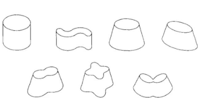
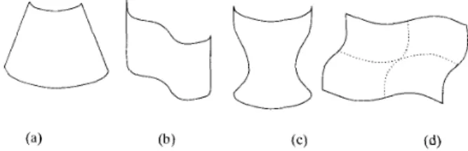
recover the local orientations of the surfaces of the objects in a scene. The basic difficulty, of course, is that an image is a 2-D projection of the 3-D scene, and hence, the 3-D structure cannot be recovered without some assumptions. In spite of the inherent ambiguities in a single view, humans are able to perceive 3-D surfaces in single images. Much effort has been devoted in the past few years to understanding this ability and has led to development of techniques such as shape from shading, shape from texture, and shape from contour (sometimes also known as shape from shape).We believe that of all the monocular cues, the shape of the 2-D contours is the most important one for the shape of the 3-D surfaces. Strictly speaking, not only is such interpretation infinitely ambiguous, but the contours can only give shape information near the contours; shape of the surface in between can vary smoothly without producing other contours. Nonethe- less, humans, when presented with contours of various and not necessarily familiar objects, perceive complete surfaces (and even solids); some examples are given in Fig. 1.
Barrow and Tenenbaum [2] have shown, by some examples, that in case of conflict between contour and shading infor- mation, humans use the contour information. Beiderman [ 11 claims that in the experiments with humans, the recognition of a full-colored image of an object is not faster than the Manuscript received August 20, 1990; revised November 12, 1991. This work was supported by the Advanced Research Projects Agency of the De- partment of Defense and was monitored by the Air Force Office of Scientific Research under Contract F49 620-90-C-0078. The United States Government is authorized to reproduce and distribute reprints for govemmental purposes notwithstanding any copyright notation hereon.
F. Ulupinar was with the Institute for Robotics and Intelligent Systems, School of Engineering, University of Southern California, Los Angeles, CA 90089-0273. He is now with the Department of Computer Engineering, Bilkent University, Ankara, Turkey.
R. Nevatia is with the Institute for Robotics and Intelligent Systems, School of Engineering, University of Southern California, Los Angeles, CA 90089- 0273.
IEEE Log Number 9205812.
recognition of the line drawing of the object. He also shows that we do not necessarily need to have any familiarity with the object in order to perceive a shape from its boundary. We conjecture that the reason for preferring shape from contour over other cues, such as shading, may be that even though shape from contour methods require some assumptions, other methods require even stronger assumptions. Shape from shad- ing methods, for example, need to assume that the reflectance properties of the surface are known, that the albedo is constant, and that the light sources are known precisely.
These observations are not to argue that only shape from contour is important but that it is an essential element in monocular perception that cannot be ignored. We believe that such an ability will also be essential for machine vision systems if they are to work with monocular images in the absence of highly specific models.
The early work on inferring 3-D structure from a 2-D shape was focused on analysis of line drawings of polyhedra [6], [4], [12], [7], [9]. In polyhedral scenes, the problem is that of segmentation and estimating orientations of faces. Recently, some papers (e.g., [17], [15]) have been published that study the projection and geometry of certain classes of curved surfaces. However, the analysis is not sufficient to recover the 3-D surfaces. Techniques for nonpolyhedral scenes have been proposed in [2], [26], [3], [20], [27], [5]. We discuss these in more detail in Section I1 and contrast them with our work later. Most of these techniques examine a single surface in the scene, whereas human perception of one surface can be strongly influenced by the perception of the other surfaces comprising the entire object.
Our technique is based on the analysis of symmetries in a scene. We show how certain symmetries can be used to infer surface orientations. We also conjecture that humans perceive only slight surface orientation information in figures lacking symmetries. Our work may be viewed as being based on generalizations of concepts that have been used previously such as by Kanade [7] for polyhedral scenes and by Stevens [20] and Xu and Tsuji [27] for curved surfaces. We believe that our method is of wide applicability. In particular, we provide a rather complete analysis for the case of “zero-Gaussian curvature” (ZGC) surfaces, but many parts of the technique also extend to nonZGC surfaces [24]. We believe that the universe of ZGC surfaces is significant (all the examples in Fig. 1 are included) and that they define a reasonable step up in complexity from planar surfaces on which much of previous work in the field has focused.
Our method assumes that clean, closed boundaries are given (or can be extracted from the real image). We do not address the issue of separating object boundaries from 0162-8828/93$03.00 0 1993 IEEE
4 IEEE TRANSACTIONS ON PATTERN ANALYSIS AND MACHINE INTELLIGENCE, VOL. 15, NO. 1, JANUARY 1993
Fig. 1. Some figures for which we readily perceive the shape from contour alone.
surface markings or other perceptual grouping operations here,
although we believe that some of the previous work in our group on this topic is relevant [13]. In addition, we believe that the specific conditions needed for an object surface to be reconstructed by our method will provide further constraints for the perceptual grouping operations when surface markings and other noisy boundaries are present.
In Section 11, we discuss previous related methods. In Section 111, we define two kinds of symmetries and discuss the qualitative shape inferences that can be drawn from them. In Section IV, we describe our technique for quantitative shape recovery of Zero-Gaussian Curvature surfaces and state our conclusions in Section V.
We assume orthographic projection throughout the paper unless specifically mentioned otherwise (in a separate paper, we have shown how many of the constraints for orthographic projection can be transformed to the case of perspective projection [25]).
In this paper, we will use gradient space to represent the
orientation of surfaces (given by their normals). To review, the normal N of a plane, ax
+
by+
cz+
d = 0 is given by the vector N = (a, b, c). This can be rewritten as ( p , q , l), wherep = a / c and q = b/c (note that this excludes cases where c = 0; however, such planes are parallel to the line of sight and are not imaged as planes under orthographic projection anyway). ( p , q ) can be thought of as defining a 2-D space (the gradient space) such that every point in this space corresponds to the normal of a plane in 3-D.
11. PREVIOUS WORK
Here, we present an overview of the important classes of previous methods. We also give our view of their strengths and weaknesses. As our method builds on some of the previous work, this section will also help provide some of the relevant background for describing our work.
These previous methods fall into two broad classes. In the first, some property of the 3-D surface is made extremal. In
the second class, which is known as constraint based, some
geometric constraints are satisfied.
A. Extrema1 Methods
In this class of methods, a measure of some desirable property, such as smoothness or compactness, is associated with each interpretation (of a curve or a figure), and the one with the best value is chosen.
Fig. 2. Shape perception: (a) smooth curve; (b) two symmetric curves; (c) two nonsymmetric curves
Barrow and Tenenbaum [2] proposed to use the smoothness of the curve as the preference criterion. Their method is not restricted to planar curves. The smoothness function they propose is an integral function of curvature and torsion of the 3-D curve. Over all possible 3-D curves that can generate a given 2-D image curve, they choose the one that minimizes the aggregate curvature and the torsion of the 3-D curve. Besides being highly sensitive to noise, this method fails to utilize structural information given in the image. For example, in Fig. 2(a), the single curve does not give any strong 3- D shape impression, but in Fig. 2(b), where another curve that is perfectly symmetric to the first one is added, a definite shape is perceived. In Fig. 2(c), two nonsymmetric curves are displayed, and again, there is no definite shape perception.
Weiss [26] has proposed a modified measure that uses curvature rather than its derivative and handles polygons in a cleaner way. For planar curves, he proposes to minimize the integral of the square of the curvature, and for polygons, he proposes using the square of the angles of corners for polygonal scenes as a minimization criteria. This method also does not utilize the structure information available in the image.
Brady and Yuille [3] used the “compactness” of a figure as their preference criterion. The measure of compactness is chosen to be ( a r e a ) / ( p e r i m e t e r ) 2 . This measure implicitly
assumes that the curve is planar. This method is insensitive to small amounts of noise and processes smooth curves and polygons in a unified way. Although this method has many nice features from a computational point of view, it does not always give answers consistent with human perception. The method correctly interprets an ellipse as being a projection of a circle, but it interprets a rectangle in the picture as a slanted square, which is not the typical human perception. In addition, when the boundary is not complete, this method is undefined. B. Constraint-Based Methods
In this class of methods, constraints on 3-D surface ori- entations are obtained by a variety of observations, with the expectation of getting unique (or a few) solutions when the various constraints are combined. In general, the constraints are based on some assumption that an observed regularity in
the image corresponds to a regularity in the 3-D scene. We briefly survey the important techniques below.
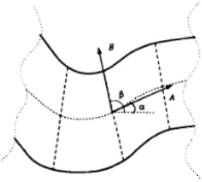
A symmetric figure in 3-D, with a straight axis and lines of
symmetry that are orthogonal to it, projects in a figure that is skew symmetric (under orthographic projection), i.e., the lines
of symmetry are no longer orthogonal to the axis but are at a constant angle to it. Kanade [7] showed that if we assume that the inverse also holds, i.e., the observed skew symmetry in the image is due to orthogonal symmetry in 3-D, then the orientation of the plane is constrained to be along a curve (a
ULUPINAR AND NEVATIA PERCEPTION OF 3-D SURFACES 5
hyperbola) in the gradient space. Kanade combined the skew symmetry constraints with a constraint that is derived from the projection of a line formed by the intersection of two planes (we call this constraint shared boundary constraint in Section
IV-A-I). The two constraints together are often sufficient to fix the orientation of the surface in the scene, and the answers given by this method appear to be consistent with human interpretation. Of course, this methods applies only when skew symmetric objects are present.
Stevens [20] studied cylindrical surfaces using the orthogo- nality property. A cylindrical surface is one where one of the principal curvatures is zero, and the lines of zero curvature (the rulings of the surface) are parallel to each other. For
such a surface, the lines of maximum curvature are planar and parallel to each other. Stevens assumes that the lines of maximum curvature are given. The rulings can be obtained from these by connecting points with the same tangent. The surface is thus covered by a grid of curves, with the property that on the actual surface, the curves are orthogonal at the points of intersection. Thus, constraints similar to those of the skew symmetry analysis can be applied. Stevens chooses to use the slant, CI and tilt, T representation’ instead of ( p . q )
representation.
As before, the constraint is not enough to give unique orientations. However, Stevens observes that slant and tilt parameters can be bounded and that the bound depends on the angle ,B between the two intersecting curves, with error in tilt approaching zero as
p
approaches T . This happensnear the occlusion boundaries of a cylindrical surface. Starting from these points, where tilt can be fixed accurately, Stevens gives a method of propagating the estimates along the lines of maximum curvature by the following formula (given without proof here):
t a n 71 t a n = t a n r 2 tan ,Ll2 (1)
where T, are the tilt angles, and
p,
are the angles betweenthe lines of maximum and minimum curvature at two points along a line of maximum curvature.
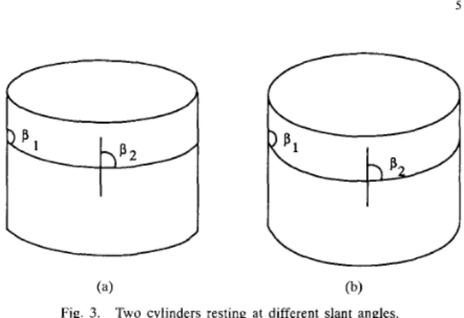
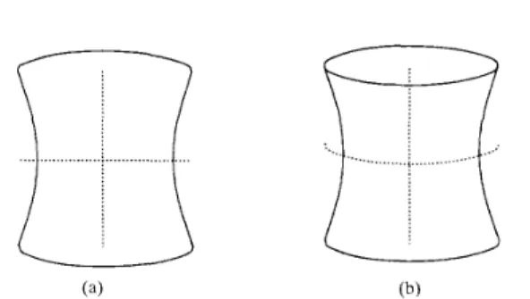
This method, however, does not always give correct results, even when a circular cylinder is given to it, as can be shown by a simple example. Consider the two cylinders in Fig. 3. The points on the limb edges for both cases have equal to
T , which give unambiguous values of zero tilt. Using Stevens
method to extrapolate along the cross section, we will get the same orientations for the midpoints of the two cylinders where
/?2 is 7rJ2, which is in clear contradiction with our perception
(which indicates that the top surface of (b) appears to be much more slanted to us then that of (a)).
Xu and Tsuji [27] have described an extension of this method for more general curved surfaces. In addition, their method does not require that all lines of curvature be given but rather that the surface be cut along these lines of curvature. Given a figure with four sides, such that two of the opposite sides are lines of maximum curvature and the other two are Orientation of a surface, having gradient ( p . q ) , can be alternately de- scribed in terms of its tdr, 7 and slant, o, which can be viewed as the polar coordinates of a point in gradient space, specifically T = arctan 9
P ’
U = arctan
Jm-
(4 (b)
Fig. 3. Two cylinders resting at different slant angles. lines of minimum curvature, they show how a net (or a grid) over the figure can be constructed with the expected property that the corresponding net on the 3-D surface is orthogonal (this construction is strictly valid only for a restricted class of surfaces). Surface orientations are first computed at special points on the net where error in tilt is small (as in Stevens’s method) and then propagated to other points on the net.
This method seems to work well in some cases but has some drawbacks. The propagation scheme for noncylindrical surfaces is only approximate, and errors can add up. In addition, it applies no test for whether the four sides of a figure could be lines of curvature, and the method may give
answers completely inconsistent with human interpretation. In a recent paper, Horaud and Brady [55] present a method for interpreting linear straight homogeneous generalized cylin- ders (LSHGC’s). Their method makes the following assump- tions: a) the axis of the LSHGC projects as the axis of the ribbon formed by the two limb contours in the image plane, b) the cross section of the LSHGC is planar, and c) the cross section is orthogonal to the axis in 3-D. Satisfying assumption b) above gives a constraint that the orientation of the cross section must be along a certain curve in the orientation space (the curve is shaped like the character “s” and, hence, is called an “s curve”). They also require that the back-projected cross section satisfy the Brady-Yuille compactness measure. If an orientation satisfies both constraints, then that orientation is chosen. They do not specify what should be done if this is not the case, although a natural extension would be to take the most compact shape constrained by the s curve. Finally, they suggest sweeping the reconstructed cross section along the 3-D axis to reconstruct the surface of the LSHGC.
This method has the attractive property that it attempts to combine the constraints from two surfaces. However, it has several deficiencies. The compactness measure can only be applied to complete cross sections. More seriously, assumption a) above is incorrect. Given the image of an LSHGC, we can choose any axis that passes through the apex of the LSHGC in the image plane and reconstruct an orthogonal LSHGC in
3-D, including the ends, that would project like the LSHGC in the image plane, as shown in the following. Take any back projection of the chosen axis, and back project the two cross sections (the top and the bottom) on any two planes orthogonal to the back-projected axis; the orthogonal LSHGC can be completed by joining the points on the cross sections such that
6 IEEE TRANSACTIONS ON PATTERN ANALYSIS AND MACHINE INTELLIGENCE, VOL. 15, NO. 1, JANUARY 1993
(a) (b) (c)
Fig. 4. Examples (a) and (c) show parallel symmetry with curved contours, and (b) shows parallel symmetry with straight contours. The dotted curves are axes of symmetry, and the dashed lines are lines of symmetry.
the lines joining these points pass through the back-projected apex. Finally, even if an axis is chosen in the image plane, the point through which the 3-D axis pierces the reconstructed 3-D cross section must be chosen in order to reconstruct the LSHGC. This point is not addressed in the Horaud and Brady paper.
In other work, Nalwa [15] has derived a symmetry condition that must be satisfied by the limb boundaries of a solid of revolution (sufficiency of these conditions is also claimed under certain general-viewing conditions). However, this paper does not show how to actually reconstruct the surface. Ponce et al. [I71 have derived properties that must be satisfied by a broader class of surfaces known as straight homogeneous generalized cylinders (SHGC’s). Again, this property by itself is not sufficient to reconstruct the 3-D surface of SHGC’s.
111. SYMMETRIES AND QUALITATIVE INFERENCES Our proposed technique is based on observations of symme- tries in figures. We believe that symmetries play an important role in shape perception; this also has been noted and used by many researchers [16, [15], [8], [ 7 ] , [20], [13]. We define two types of symmetries that we call parallel symmetry and skew symmetry and discuss how they can be used to infer surface shape.
A. Parallel and Skew Symmetries
For curves to be symmetric (parallel or skew), certain point- wise correspondences between two curves must exist. We will call the lines joining the corresponding points on the curves the lines of symmetry, the locus of the midpoints of these lines the axis of symmetry, and the curves forming the symmetry as the curves of symmetry.
1) Parallel Symmetry: Consider two curves
Xi(s)
= (zi(s),yi(s)), for i = 1 , 2 , parameterized by arc length s. Let 8i (s) = arctan( (dyi( s ) / d s ) /(dz;
( s ) / d s ) ) . Then, XI (s) and X z ( s ) are said to be parallel symmetric if there exists a correspondence function f (s) between them such thatfor all values of s for which
X1
andX z
are defined, and f ( s ) is a continuous monotonic function. Note that computing symmetry between two curves using this definition requires estimating the function f ( s ) as well. A useful special case is when f ( s ) is restricted to be a linear function. In that case, the symmetry condition becomesOi(s) = 62(as
+
b ) (3)(a) (b)
Fig. 5 . Example (a) shows skew symmetry with curved contours, and (b)
shows skew symmetry with straight contours. The dotted curves are the axes of symmetry, and the dashed lines are lines of symmetry.
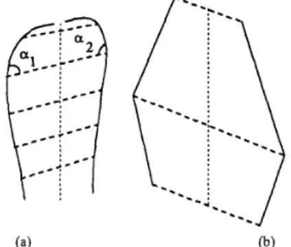
where a and b are constant ( a may be thought of as a scale parameter). Some examples of parallel symmetry are given in Fig 4; the correspondence function f ( s ) is linear for (a) and (b) but not for (c). Note that the above definition of parallel symmetry also holds for curves consisting of straight lines and corners as in Fig. 4(b).
2) Skew Symmetry: In this symmetry, the point-wise cor- respondence should be such that the axis of the symmetry is straight, and the lines of symmetry are at a constant angle (not necessarily orthogonal) to the axis of symmetry. Skew symmetry was first proposed by Kanade [7] and used in the analysis of scenes of polyhedral objects.
Ponce [I81 has given point-wise conditions for two curves to be skew symmetric. We state these here without proof. For the case when the lines of symmetry are orthogonal to the axis of symmetry, the criterion for the two curves X l ( s ) and
X 2 ( s ) to be skew symmetric is
4 ( s ) = - K 2 ( S
+
b ) (4) where ~ ( s ) is the curvature, and b is the offset. In general, let a i ( s ) be the angle between the line of symmetry and thetangent to the curve
i
at the corresponding points. Then, the necessary condition for the two curves to be skew symmetric is & I ( $ ) s i n ( a ~ ( s ) ) ~ = -Q(S+
b ) sin(aZ(s+
b ) ) 3 ( 5 )An example is given in Fig. 5(a). The above conditions are only valid for curves and not for lines, that is, curvature should be nonzero. For lines, the first definition of skew symmetry can simply be applied as two lines are skew symmetric if another set of two lines that joins the end points of the given lines are parallel to each other. In this case, the two new lines are the lines of symmetry, and the line joining the end points of these lines is the axis of symmetry. A n example of skew symmetry for straight lines is given in Fig. 5(b).
We believe that these two symmetries are major sources of information for extracting shape from contour. We discuss this process next.
B. Qualitative Shape Inferences from Symmetries
We now describe some qualitative inferences about the shape of surfaces from their symmetries. We also prove some
ULUPINAR AND NEVATIA PERCEPTION OF 3-D SURFACES
of the inferences that we make. We use the assumption of general viewpoint defined as the following:
Definition 1-General Viewpoint: A scene is said to be
imaged from a general viewpoint if perceptual properties of the image are preserved under slight variations of the viewing direction.
Specifically, the perceptual properties we are interested in are straight lines, parallelism of lines, and the symmetry of Here, we discuss the interpretation of individual surfaces
independently. In an object, of course, several surfaces may be visible, and their interpretations must be mutually consistent. This can provide a mechanism for either reinforcing individual surface interpretations or choosing among possible multiple interpretations for an individual surface.
It will be useful to consider figures as belonging to one of the following three classes:
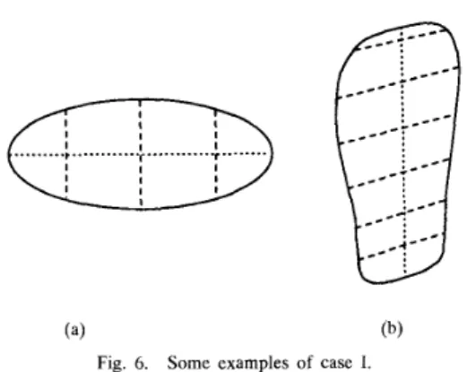
I ) Case I: Here, one skew symmetry covers the entire
boundary of the surface. We allow more than one alternative
description for a figure (Fig. 6 shows two examples). For
example, the ellipse in Fig. 6 can be described as being skew symmetric about any axis that passes through its center, and all symmetries include all the points on the ellipse boundary.
Surfaces belonging to case I are generally perceived to be planar. We prove that if a contour belongs to case I bounded by nonlimb edges, then the contour has to be planar under the assumption of general viewpoint and if the correspondence is static with respect to changing viewpoint. Limb edges (or limbs) of a surface are generated by points on the surface whose normal is orthogonal to the viewing direction. Such an edge changes its position on the surface as the viewpoint changes. Nonlimb edges, on the other hand, do not change their position on the surface as the viewpoint moves; they include creases and wireframes.
Lemma 1: A 3-D skew symmetric figure projects as a
skew symmetric figure under orthographic projection.
Proof: It is a direct result of the property of the or-
thographic projection that parallel lines project as parallel lines and that midpoints of lines project as midpoints of the projected lines. Therefore, the 3-D lines of symmetry project as the lines of symmetry on the image plane, and the projection of the 3-D axis is the line joining the midpoints of the lines of symmetry on the image plane.
Theorem 1: If a 3-D contour formed by nonlimb edges
produces a skew symmetric line drawing in the image plane such that the 3-D correspondence is invariant’ under small perturbations of the viewpoint, then the 3-D contour must be planar (under the assumption of general viewpoint).
Proof: Since the 3-D correspondence is invariant with
respect to variations of the viewpoint (that is, the projection of the same set of 3-D points correspond from different viewpoints) then, the assumption of general viewpoint implies that parallel lines in the image plane must be the projection of parallel 3-D lines; otherwise, they would not project parallel from nearby viewpoints. Therefore, we conclude that the 3-D curves.
*We thank Dr. V. Nalva for pointing out this assumption, which was omitted in an earlier version of the paper.
(a) (b)
Fig. 6. Some examples of case I.
lines, say l i , that project as the lines of skew symmetry on the image plane must be parallel to each other in 3-D because lines of skew symmetry are parallel to each other in the image plane. The axis of symmetry in 3-D, which can be obtained by joining the midpoints of the 3-D lines l i , must be straight because its projection on the image plane, which is the axis of skew symmetry, is straight. Therefore, the lines li have to lie on a plane because they are parallel to each other, and a single line, which is the 3-D axis of symmetry, intersects them. Hence, the 3-D contour, which encloses the lines l,, is Lemma 1 shows that planar skew symmetric figures project as skew symmetric figures on the image plane. Theorem 1 shows the reverse is also true under the stated conditions. We conjecture that invariance of the correspondence is not necessary but have not proved it.
Note that if the 3-D contour forming the skew symmetry on the image plane is a limb edge, then the 3-D contour could be nonplanar. For example, limb edges on surfaces of revolution produce an orthogonal skew symmetry [15]. Generally, such surfaces also produce a parallel symmetry together with skew symmetry, and they belong to case 11, which is defined below.
Case 11: Here, the boundary of the figure is covered by
exactly two symmetries, and furthermore, at least one of them must be a parallel symmetry. We will argue that the case I1 figures are the ones that give us the most information about the surface shape and that such cases are common in everyday scenes. Fig. 7 shows some examples of this case. We will show that if one of the two symmetries is a skew symmetry with straight curves of symmetry (as in Fig. 7(a) and (b)), then the surface must be a zero Gaussian curvature surface. Otherwise, if the curves of skew symmetry are not straight or have two curved parallel symmetries, then we perceive a doubly curved surface (i.e., both of the principal curvatures are nonzero). Surfaces of revolution are such cases where the limb boundaries project as orthogonal skew symmetry as shown in Fig. 7(c). A double bent paper-like surface, which is shown in Fig. 7(d), illustrates this case with two parallel symmetries.
I ) ZGC Surfaces: A zero Gaussian curvature (ZGC) sur- face is one where the the Gaussian curvature (the product of the maximum and minimum curvatures) of the surface is zero everywhere. Cylinders and cones are examples. These surfaces are also called developable surfaces since they can be generated from a piece of paper by rolling andlor bending
8 IEEE TRANSACTIONS ON PATTERN ANALYSIS AND MACHINE INTELLIGENCE, VOL. 15, NO. 1, JANUARY 1993 without cutting. Lines of minimum curvature for a ZGC
surface, which are also called rulings, are straight, i.e., it is possible to embed straight lines on a ZGC surface along these rulings.
The following theorem asserts that case I1 figures satisfying specific properties must have ZGC along its skew symmetry contours.
Theorem 2: If a surface generates one parallel symmetry
and one skew symmetry, with straight curves of skew sym- metry on the image plane, and the straight curves of skew symmetry are also the lines of symmetry for the parallel symmetry, then the Gaussian curvature of the surface must be zero along the curves of skew symmetry.
Proof: There are two subcases, depending on whether
the curves of skew symmetry are limb edges or not.
a) The straight curves of skew symmetry are produced by limb edges: In this case, just the straightness of the limb is sufficient for the surface to have ZGC along the limb. This can be inferred as a special case of theorem given by Koenderink
[lo].
We give an alternative proof here that does not need the additional assumptions used in Koenderink’s proof. Let the surface X ( U . U ) be parameterized such that a U parameter curve is along the limb boundary for 71 = U , . Since the curve X ( u . v , ) is along the limb boundary and the projection of this curve is straight, the surface normalJV
along this curve is constant, that is,N?,(u.
o,) = 0. This condition isa sufficient condition for the Gaussian curvature of the surface along the X ( U . U , ) to be zero. The Gaussian
curvature K of a surface is given by
where L ,
hl.
N are the coefficients of the second fun- damental form of the surface, and E . F. G are thecoefficients of the first fundamental form. The equations of these coefficients are given in (30). Particularly, the coefficients L and M can be written as
Since N(u,w,) = 0, the Gaussian curvature K must be
zero along the limb.
The above proof does not require the assumption of general viewpoint; hence, it only shows that along the curve of the limb boundary, the surface has ZGC. With the assumption of general viewpoint, we conclude that an open region surrounding the limb boundary also has ZGC.
The straight curves of skew symmetry are cut edges. Consider Fig. 8, where a pair of parallel symmetric curves on a ZGC surface cut along a ruling is shown.
Since, in the image plane, the tangents t l and t 2 of the top and bottom curves are parallel; by the assumption of general viewpoint, they must be parallel in 3-D. In addition, since the skew symmetry curves (one of which is the ruling in Fig. 8) are straight on the image plane, the 3-D corresponding curves must also be straight, that is,
Fig. 7. Examples of case I1 surfaces: (a) and (b) are ZGC surfaces and
( e ) and (d) are doubly curved surfaces.
the surface embeds straight lines. Therefore, the surface can locally be represented as a ruled surface having
X ( U . U ) = f ( 7 l )
+
ug(v) (8)where f ( v ) and g ( u ) are arbitrary vector functions of the parameter 1: only. The vector function g(v) indicates
the direction of the ruling that are also the U parameter
curves. The normal of this surface is
For Fig. 8, let the dotted line (ruling) be the cut boundary for 71 = I ’ ~ ] , and let J%> ( U 1 . U,) and h r 2 ( u 2 . 11,) be the
normals of the surface at points where the ruling inter- sects the parallel symmetry curves. Since the tangents
tl and t 2 are the same and, of course, the tangent of the
ruling is constant along it, the surface normals
NI
andJ ~ Z , which are the cross products of tl and t 2 with the tangent of the ruling, must be the same, that is
where indicates parallelism of the vectors. Then, we have that either 111 = u2 or the three vectors
f ‘ . g ‘ . g are dependent. Clearly, u1
#
u2; therefore,f ’ . .9’> g are dependent, and hence, the surface normal
.A* is independent of the TL parameter curve, that is,
&‘(U. IS,) = 0. As in the case (a) above, this condition is sufficient so that the Gaussian curvature of the surface
0
2) Generulizution: If we assume that the type of the surface
does not change as we go from its boundary to the inside, then
we conclude that the whole surface must be a ZGC surface if it satisfies the property given in theorem 6.
This generalization may appear to be a rather sweeping one. However, it is no more so than the common assumption that a polygonal line drawing corresponds to polyhedral objects.
It follows that if the parallel symmetry has a linear cor- respondence function, then the surface is conic, and if the correspondence function is an identity, then the surface is cylindrical. We now show how we can infer the rulings and the cross sections of the ZGC surface. Rulings are the lines along
which the curvature of the surface is zero. Cross sections are the transverse (not necessarily orthogonal) curves, specifically, the curves that project into parallel symmetric curves. We first give a theorem that is key to inferring properties of cross sections and rulings.
LJLUPINAR AND NEVATIA: PERCEPTION OF 3-D SURFACES
Fig. 8. ZGC surface cut along the “ruling.”
Fig. 9. Objects with cross sections having (a) only one skew symmetry and (b) two skew symmetries
Theorem 3: Curves obtained by intersecting a ZGC sur-
face with two parallel planes are parallel symmetric such that the lines of symmetry are the rulings of the surface.
The proof of this theorem is given in Appendix A-1. Note that the reverse of this theorem, that parallel symmetry curves
must come from parallel planar cuts, is not valid. In Appendix A-2, we show that lines of maximum curvature that are not
necessarily planar can also be projected as parallel symmetric curves. However, we believe that it is reasonable to infer that parallel symmetry curves are planar, unless we have evidence to the contrary. In general, lines of curvature of a ZGC can be very complex, and it is unlikely that an observed surface would be cut in this way. If the curves are neither planar nor along the curves of maximum curvature, it is quite difficult to obtain parallel symmetry. For example, in order to obtain parallel symmetry for a conic surface (a subcase of ZGC surfaces) by cutting with nonplanar cross sections, the cuts must be translated along the axis of the cone and scaled exactly with the scaling function of the cone.
Our interpretation does allow for piecewise planar cross sections, as indicated by multiple skew symmetries. Fig. 9
shows an example. The cross section of the object in Fig. 9(a) has a single skew symmetry and is perceived as planar, whereas the cross section of the object in Fig. 9(b) has two skew symmetries, and the perception is that the cross section has two planar parts, that is, if the cross section has multiple skew symmetries, then it will be piecewise planar such that each planar section has one skew symmetry.
3) Recovering Rulings: We can infer the rulings of the surface by joining the corresponding points on the two curves forming the parallel symmetry by straight lines, as shown in Fig. 4(c) (the corresponding points on the two curves have the
9
Fig. 10. (a) Figure with two skew symmetries: (b) addition of an extra curve clarifies the perceived shape
not change along a ruling (this is also proved as a byproduct of the above proofs in the Appendix). Therefore, if we find the orientation of the surface at a single point on a ruling, we can extend it along the ruling. A quantitative analysis for ZGC surfaces is presented in Section IV.
Case 111: This class includes all remaining cases. Three interesting subclasses occur here.
~
same tangent). Note-that the orientation of a ZGC surface does straint relates the orientation of the points on two inter- a) The contours satisfy specific properties of some special
objects (e.g., straight homogeneous generalized cylinders
[17]. [23]), in which case, the analysis can use these
special properties.
b) We hypothesize the presence of some boundaries not present in the image to convert the figure into case I,
11, or III(a) above. For example, consider Fig. lO(a) with two skew symmetries. Note that we have no strong feel for the 3-D shape of this surface. However, if we assume that there is one missing boundary that would introduce a parallel symmetry (and an additional skew symmetry) as shown in Fig.
lo@),
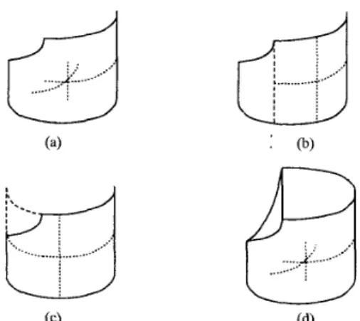
the surface shape becomes very distinct. Of course, more than one such construction may be possible, where each gives an alternative interpretation; some constructions may be preferable according to some heuristic criteria.Another interesting case is where two symmetries cover most of the boundary but not all of it; an example is given in Fig. l l ( a ) . Here, two choices are available. Either we can inscribe a smaller figure inside the larger one, or we can extrapolate some of the boundaries to meet the requirements of case 11. The two choices are shown in Fig. 1l(b) and (c). Note that the extrapolation is preferred if the “top” surface is also shown, as in Fig. 1 1 (d).
c) All other cases. Such figures are out of the scope of this paper. We also believe that such shapes are difficult for humans to perceive.
IV. QUANTITATIVE SHAPE RECOVERY
We now describe our technique of quantitative shape re- covery. We will focus on ZGC surfaces, although some of our analysis applies to more general cases. Remember that presence of ZGC surfaces is indicated by observing the properties given in Theorem 2.
Our method is dependent on the use of three constraints:
10 IEEE TRANSACTIONS ON PAITERN ANALYSIS AND MACHINE INTELLIGENCE, VOL. 15, NO. 1, JANUARY 1993
Fig. 12. Two curved surfaces meeting at a curve I?.
.
((P2(S), 92(s), 1)-
(Pl(S), 41(s), 1)) Fig. 11. (a) Face of a cylinder with a clipped corner; (b) parallel symmetry = Oz’(s)(p2(4 - Pl(S))+
y’(s)(q2(4 - 41(s)) = 0. (11)cover only part of the surface; (c) top curve is extended for the parallel symmetry to cover the whole face; (d) top of the surface is also included
setting surfaces. A simpler constraint is obtained if we
can assume the planarity of the curve produced by the intersection of two surfaces.
Inner surface constraint (ISC): This constraint restricts the orientation of the neighboring points on a surface. Orthogonality constraint (OC): This constraint uses the assumption that the lines of parallel symmetry and the axis of parallel symmetry (i.e., the rulings and the cross sections) are orthogonal to each other in 3-D.
We first describe these constraints in detail and then discuss the combination of these constraints for different classes of ZGC surfaces. These constraints, in general, are not sufficient (even though a sufficient number of equations are obtained) to give unique surface orientations; they typically leave one degree of freedom unconstrained. To fix this degree of free- dom, we use the shape of the parallel symmetry curves (or the cross sections).
A. Constraints
We now give some constraints that derive from observations of the symmetries and other boundaries in the image. We formulate three constraints discussed in subsections below and then discuss how to combine them.
I ) Curved Shared Boundary Constraint (CSBC): This con-
straint relates the orientations of the two surfaces on opposite sides of an edge. The planar version has been used since the early days of polyhedral scene analysis [12]. Shafer et al. [19] extended it to the case of intersection of curved surfaces.
Consider two surfaces X I ( U , U ) and X2(u, U ) meeting at a
curve
r(s)
= (z(s),y(s),z(s)) as in Fig. 12. Let N l ( u , v )and
N2(u,
w ) be the normals of X 1 and X2, respectively. Along the curver(s),
we can represent the normals N1 andNz as N ; ( s ) = Ni(ui(s),wi(s)). Let the normals
Ni(s)
be represented in in p-q space as N ; ( s ) = ( p i ( s ) , q i ( s ) , 1). Then,the curved shared boundary constraint (CSBC) states that along the curve
r(s),
the orientation of the surfaces X I andX2 are constrained by the tangent ( ~ ’ ( s ) , y’(s)) of the image of the curve
r(s)
by the following equation:(+>, Y’(S), z ’ ( s ) )
Proof of this constraint is omitted but follows from results given in [19]. A stronger constraint can be obtained if we can assume that the intersection curve is planar. Say
r
lies in a plane with orientation(pc.qc).
With the assumption of planarity, the constraint equation becomesZ ’ ( S ) ( P c - d s ) )
+
Y ’ ( S ) ( ! I c - d s ) ) = 0. (12) For ZGC surfaces, we will assume that the parallel symmet- ric curves (or cross sections) are planar (based on an argument given in Section 111-B-2).2) Inner Surface Constraint (ISC): The inner surface con- straint restricts the relative orientations of the neighboring points within a surface. For ZGC surfaces, the image of the rulings of the surface is used to constrain the surface orientation of neighboring points.
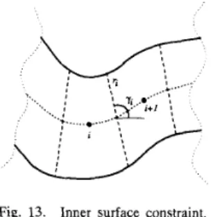
Let X ( u , w) = ( ~ ( u , U), y ( u , U), z ( u , w ) ) be a ( U , w ) para- metric representation of the surface X , and let w be along the direction of minimum curvature (rulings for ZGC surfaces). We can form an orientation function in terms of the parameters
u and w : O ( u , w) = ( p ( u , U), q(u, U)). The inner surface con-
straint (ISC) states that for a constant value of the parameter w , say vo, as the parameter u changes the direction of the function 0 in the p - q plane, 0, = ( p , , qu) should be orthogonal to the direction of the image of the tangent of the rulings, that is, the lines of symmetry (zv, yv) under orthographic projection, that is
( P u , 4 u )
.
(xu, Y v ) = 0p u z v
+
q u y u = 0. (13)The proof of this property is given in Appendix A-3. Geometrically, the ISC can be described as follows: As we move along the axis of parallel symmetry (the u parameter curve), the surface orientation should move in the p - q plane in a direction orthogonal to the image of the rulings (the lines of parallel symmetry). For example, for cylindrical surfaces, this ISC curve is a straight line since all rulings are parallel
ULUPINAR AND NEVATIA: PERCEPTION OF 3-D SURFACES 11
Fig. 13. Inner surface constraint
to each other. Note that this constraint does not require any regularity assumptions about the contour.
The above equation expresses the inner surface constraint in a continuous domain. In the discrete domain, suppose the surface orientation is to be computed at n points for a ZGC
surface (these n points are along the axis of the parallel
symmetry since the surface orientation for a ZGC does not change along the rulings). We have 2n unknowns ( p i , q i ) for
n points. This constraint provides us with n - 1 constraint equations as shown below.
between the ith and (i
+
1)st points make an angle yi with the horizontal, as in Fig. 13. The constraint equation relates the change in orientation along the axis of symmetry ( p U , q U ) to the tangent of the ruling(xu,
yu). Here, the tangent of the ruling is(xu,
y u ) = (cos(yi), sin(yi)), and the derivatives ( p u , q u ) can be approximated by thefirst-order difference as ( p z l , q z l ) = (pi+l
-
p ; , q ; + l-
4;).Substituting these in (13) gives Let the image of the ruling
(pi+l -pi) cos(yi)
+
(qi+l-
q i ) sin(y;) = 0. (14)3) Combination of ISC and CSBC: In the discrete domain,
we need to quantize ( p ( s ) , q ( s ) ) as ( p i , q i ) and estimate
( d ( s ) , y’(s)) from the image of
r(s),
which is ( x ( s ) , y(s)) under orthographic projection. If the ZGC surface is to be described at n points, then there are 2n+
2 unknowns, 2n for the surface orientations ( p i , q i ) and 2 for the cross section plane ( p c , q c ) . This constraint provides us with n constraint equations. By using the CSBC in conjunction with the ISC, we get 2n-
1 equations. This leaves us with three degrees of freedom for describing a ZGC surface totally.The two constraints are shown graphically in Fig. 14. A ZGC surface (a frustrum) is shown in (a) with rulings and the axis of the symmetry marked on the surface. The ISC curve is shown on the p - q plane. Here, the section of the ISC curve from the point ( p i , q i ) to ( p i + l , q i + l ) is orthogonal to the ruling ri. The straight lines on the p - q plane are the CSBC’s such that at each point i, the tangent of the axis of symmetry (the dotted curve on the surface) is orthogonal to the corresponding CSBC line on the p - q plane. Three parameters required to fix all the orientations ( p i , 4;) are the orientation of the plane containing the intersection curve ( p c , q c ) and
the quantity shown as d in Fig. 14, which we call the angle parameter. The angle parameter can be described as distance of the ISC curve from the point ( p c , q c ) , which corresponds to an angle in 3-D. Specifying the length of one of the CSBC lines is enough to fix the angle parameter d.
Fig. 14. Three degrees of freedom present p c , q c , d in a ZGC surface after applying the constraints ISC and CSBC.
Fig. 15. Two cylinders (a) cut along the curves of maximal curvature; (b) cut in an arbitrary direction while preserving parallel symmetry. Now, we have the perception of an elliptical cylinder.
4) Orthogonality Constraint (OC): We will assume orthog- onality between the axis of parallel symmetry and the lines of parallel symmetry. This is equivalent to slicing the surface along rulings to obtain thin skew symmetric planar strips and assuming that these strips are orthogonally symmetric in 3-D, as in Kanade’s analysis for polyhedra [7]. This preference is
illustrated in Fig. 15, where in (a), we see a circular cylinder, but in (b), we see an orthogonal elliptic cylinder rather than a slanted cylinder. Note that for ZGC surfaces, where the lines of symmetry are the rulings of the surface (or the lines of least curvature), the orthogonality constraint implies that the cross sections must be along lines of maximum curvature. This is, in general, in conflict with our drive to to perceive the cross section as being planar (except for cylinders and cones). We discuss how to resolve these conflicting constraints in Section For a ZGC surface, say, the tangent of the axis of symmetry, makes an angle a with the horizontal, and the ruling makes
an angle ,B at some point on the surface, as in Fig. 16. Let the normal of the surface be N = ( p , q , 1) at that point. Since the
3-D tangent vectors A and B are on the tangent plane of the surface, they can be represented as
IV-B.
A = ( c o s ( a ) , s i n ( a ) , p c o s ( a )
+
qsin(a))B
= ( ~ O ~ ( P ) , ~ i ~ ( P ) , P C O ~ ( ~ )+
4 W P ) ) . (15) and from the orthogonality of the 3-D vectors A and B, we get A + B = 0 orcos(a -
p )
+
(p cos a + q sin a)(pcosp
+
q sin ,f?) = 0. (16) This is the equation of a hyperbola in the p - q space, con- straining possible orientations for the surface normal N .In discrete domain, we need to digitize a,
p,
p , and q above as ai,pi,
pi, qi for each point on the axis symmetry. This constraint provides us with n equations if the surface orientation is to be computed at n points.12 IEEE TRANSACTIONS ON PATTERN ANALYSIS AND MACHINE INTELLIGENCE, VOL. 15, NO. 1, JANUARY 1993
Fig. 16. Orthogonality constraint. B. Combining the Constraints
The three different constraints of the previous sections provide 3n - 1 constraint equations for n points producing 2n
+
2 unknowns (including ( p c , 4,)). This suggests that the system of equations is overconstrained (for n>
3). Thus,in general, it may not be possible to find an interpretation for the contours such that the surface obeys all the given constraints exactly. Furthermore, the orthogonality constraints and planarity of cross sections assumed by CSBC are usually in conflict, as discussed in Section IV-A-4. However, for special but important cases, these sets of constraints are dependent and may give a unique answer or even leave one degree of freedom unconstrained.
1) Cylindrical Surfaces: A cylindrical surface is a ZGC
surface for which rulings are parallel to each other in 3- D. A n example is given in Fig. 17(a). Let this surface be parameterized by X ( U , U) = ( x ( u , U), y(u, U), Z ( U , U)) such
that U is along the axis of symmetry, and U is along the rulings. As we move along the axis of symmetry, let the angle between the tangent of the axis of symmetry and the horizontal be a(.).
Note that a is a function of U only, and let the angle between
the ruling and the horizontal be
p,
as in Fig. 17. Note that, since all rulings are parallel, /3 is constant. We can always rotate the coordinate system to makep
equal to n/2, as inthe figure. With these angles, we have
X , = ( x u , y,, z,) = (cos a , sin a , z,)
x,
= ( X v , y v , 2,) = ( C O S P , s i n p , 2,) = (0,1, 2,). (17) Our purpose is to compute the surface orientation( p ( u ) , q ( u ) ) along the axis of symmetry. Applying the inner surface constraint in (13) gives
p , z ,
+
quyv = 0*
q(u) = q,(constant) (18)(a) (b)
Fig. 17. (a) Cylindrical surface with axis of symmetry and the rulings marked; (b) constraints ISC, CSBC, and the orthogonality for the cylindrical surface.
given by orthogonality, as given in (16). Since
p
= 7r/2, we haves i n ( a ( u ) )
+
q,p(u) C O S ( ( Y ( U ) )+
y,2 s i n ( a ( u ) ) = 0. (20) Substituting p ( u ) , by (19), in the above equation givessin(cr(u))(l+ qoqc)
+
p , cos(a(u)) = 0. (21) Since the above equation is equal to zero for all values ofU , then we have both p , = 0 and
1
+
qoq, = 0*
qo = -l/yc. (22) With the orthogonality constraint, we have p , = 0 and qo = - l / q , , leaving q, as a variable, that is, the three constraints CSBC, ISC, and OC are satisfied for a cylindrical surface, and still one degree of freedom, namely qc, remains. In Section IV-C, we describe a method to estimate qc. The method uses the shape of the parallel symmetry curves.2) Circular Cones: A circular cone is a linear straight
homogeneous generalized cylinder (LSHGC), whose cross sec- tion is a circle. The importance of circular cones is that these are the only ZGC surface that have a unique (two including the Necker's reversal) solution to the three constraints (ISC, CSBC, and OC) given before. In [22], we have analyzed the image of a cone under these constraints, and a unique solution, which is also in agreement with the assumption that the ellipse of the cross section in the image plane is the projection of a circle in 3-D, is found.
3) General ZGC Surfaces: For surfaces other than cylin- drical surfaces and the circular cone, the three constraints cannot be satisfied exactly. We believe that in most cases, the planarity assumption is stronger than the orthogonality assumption. Therefore, the following process tries to maximize the orthogonality while keeping the constraints ISC and CSBC satisfied exactly.
that is, the ISC curve is a horizontal line on the p - q plane as shown by dotted line in Fig. 17(b).
Say that the orientation of the cross-section plane is ( p c , q c ) . Then, the curved-shared boundary constraint gives
%(Pc - P ( U ) )
+
yu(qc - 40) = 0sin(a(u))(qc - 40) + p , .
As discussed in Section IV-A-3, there are three degrees of freedom left for reconstructing a ZGC surface. The free variables are ( p c , q c ) and d. We choose the values for these free variables that minimize the orthogonality error
COS(4U))(PC - P ( U ) )
+
sin(a(u))(qc - 40) = 0 (19)COS(Q('IL))
P ( U ) =
n
that is, if we fix pc,qc and qo, then the surface's orientation
ULUPINAR AND NEVATIA PERCEPTION OF 3-D SURFACES 13
t '
I.. " Iwhere 0; is the angle between the two 3-D vectors ( A and B )
in Fig. 16, whose projection on the image plane make angles
a; and with the horizontal. cos0; is given by
Here, ( p i , q i ) are dependent on (p,, q,) and d as given by constraints ISC and CSBC. We want to maximize the or- thogonality by minimizing the above function 2 for (pcl q,)
and d. We can convert this problem into a 2-D minimization problem by associating a d value to each choice of ( p , , q , ) that minimizes Z.
Unfortunately, for a general conic surface, the global mini- mum for
=
occurs when ( p c , q,) = (0,O) and d = m. This is an infeasible interpretation. However, function Z, in terms of (pcl q c ) , has a "valley" of local minima (passing through the origin of the p-q space), and the valley is typically a straight line. Any choice of (p,,qc) along this valley is essentially equally acceptable, i.e., we have one degree of freedom to fix. In Section IV-C, we discuss how to choose a specific value of (pel q c ) on this line using the shape of the cross section.C. Estimating ( p c , 4,)
As discussed in Section IV-B, the previous three constraints
(ISC, CSBC, OC) leave one degree of freedom such that the orientation of the cross section plane ( p c . q c ) is constrained to be along the minimum line of the function E. It is expensive to compute this minimum line. Instead, we use the following gradient descent algorithm to compute (p,, q c ) :
1) Choose a starting line 1, passing through the origin in the p-q space in the direction of the skew symmetry axis. Set the current line to 1 = 1,.
2) Compute the (pcl q,) for the line 1 using the method described below.
3) Compute the value of E for ( p c , q c ) , and check if ( p c , q c ) is along the minimum line of Z by repeating the above process for lines
&SO
degrees off the line I , and by comparing the Z values for these lines.4) If ( p c , q , ) is along the minimum line of E, then stop. Otherwise, choose another line by rotating the line 1 by Sf3 degrees in the direction of descending Z, and go to
step 2.
1) Computing ( p c , q c ) Given a Line 1: We rotate the coor- dinate system such that the line 1 is aligned with the q axis of the p-q plane. Then, we have p , = 0, and qc is the unknown quantity.
To fix qc, we use the shape of the cross section. We propose a method based on perceptual properties rather than on mathematical constraints.
Our method is based on the following observations of human perception:
We prefer compact shapes (as also observed in [3]).
We prefer medium slant to very high or very low slant. We have a large range of uncertainty for the perceived Based on these observations, we propose a two-stage method for determining qc. First, we estimate a value for qc, and then,
slants.
(a) (b)
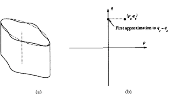
Fig. 18. (a) Cylindrical object and the ellipse fitted to the cross section; (b) orientation ( p c . q , ) that would make the ellipse a circle and its projection on the q axis gives q c , which is first approximation to q c .
we update it with a bias toward 45". For the first estimation, an ellipse is fit to the cross section and then backprojected to an orientation that makes it a circle (apart from being much faster, this has an advantage over the ( a r e a ) / ( p e r i m e t e r ) '
measure used by Brady and Yuille [3] in that it does not require that closed contours be given). Since this is a rather heuristic approach, we have performed a psychological study validating this approach. The details of this study are provided in [21], and a summary of the results is given at the end of this subsection. The two steps are described in detail below.
2) First Estimation of qc: An ellipse-fitting process is uti- lized as a first approximation for qc. An ellipse is fit to the cross section contour, and then, the orientation of the circle (pel q e ) that would be projected as the fitted ellipse is projected on the
q axis on the p-q plane to obtain the first approximation of qc; call it qe. Fig. 18 shows an example. Note that there are two values of (pel q e ) that make a circle project as the ellipse in the image plane. These correspond to Necker's reversal. We choose the one that gives a solid shape interpretation in preference to the one that gives the interpretation of a hole.
The behavior of the method is dependent on the choice of the ellipse fitting algorithm used. We have experimented with two different ellipse fitting algorithms. The first one is based on the scattering of the boundary points. A covariance matrix of the equally spaced contour points is computed by
where (z;,yi) are the equally spaced boundary points, and
(?fly)
is the mean. The scattering of these contour points is given by the eigenvalues e l and e2 of the covariance matrixC. Say that the unit vectors z11 and v2 are eigenvectors of
C corresponding to el and e 2 , respectively. Then, we can
approximate the cluster of points (xi, y;) with an ellipse whose major and minor axes are in the directions w l and w2 with magnitudes and
@.
This method is quite robust when the contour is closed. However, for open contours, the method consistently underestimates the eccentricity of the ellipse.The second method is a regular least squares fit of the parameters of the quadratic representation of the ellipse to the boundary points. This method is robust when the contour is similar to an ellipse whether it is closed or not but may