PAIRS TRADING IN XU100
ÜMĐT KIVANÇ BATTAL
106622003
ISTANBUL BILGI UNIVERSITY
INSTITUTE OF SOCIAL SCIENCES
MASTER OF SCIENCE IN ECONOMICS
UNDER SUPERVISION OF
ASST. PROF. DR. ORHAN ERDEM
1
PAIRS TRADING IN XU100
IMKB 100 DE ĐKĐLĐ ALIM SATIM
ÜMĐT KIVANÇ BATTAL
106622003
ASST. PROF. DR. ORHAN ERDEM……….
ASSOC. PROF. DR. EGE YAZGAN………..
ASST. PROF. DR. KORAY AKAY……….
Tezin Onaylandığı Tarih:……….
Toplam Sayfa Sayısı: 44
Anahtar Kelimeler
Keywords
1) Đkili Alım Satım
1) Pairs Trading
2) Đstatistiksel Arbitraj
2) Statistical Arbitrage
3) Özsermaye
3) Owner’s Equity
4) Koentegrasyon
4) Cointegration
2
ABSTRACT
In this paper, we have studied market behavioral (market friendly) pairs trading. The idea in pairs trading is basically to determine the long run relationships between the prices of two financial assets, and take the advantage of the short run deviations from this relationship. Pair trading is based on the idea that if historical price series of some chosen stocks have a stable relationship in the long run, any deviation from the long run relationships between the assets should be treated as mispricing between these two stocks and it suggests having a long position in the undervalued assets by selling the overvalued one. In this study a market behavioral (market friendly) pairs trading strategy is used to examine the empirical results in IMKB. In this paper there were some risk controls to improve the performance of the strategy. Some restrictions were imposed while choosing the appropriate stocks for pair trading. First of all, we were only interested in stocks whose companies are financially doing well. Secondly, the pairs are formed by the stocks which are operating in the same sector. Thirdly, unlike the classical pair trading strategies, we did not carry positions on the stocks all the time; instead, there were some periods of times that we only held cash but nothing else. When economic climate was not appropriate, we chose to wait in cash. The indicator DI+/DI- was used to check whether economic climate is appropriate for investing in stocks. Moreover, our model was not a static model but a dynamic one. Finally, even though, the return results were significantly good in the market friendly pairs trading strategy, investors should keep in mind that making investment on a stock exchange market carries some risks and it is not possible to build a totally risk-free strategy.
ÖZETÇE
Bu çalışmada market dostu ikili alım satım yöntemi incelenmiştir. Đkili alım satımdaki temel düşünce, uzun dönemde birlikte hareket eden iki hisse senedi bulmak ve kısa dönemde bu iki hisse senedinin uzun dönemli ilişkisinde bir bozulma olduğunda bundan faydalanmaktır. Đkili alım satımda önemli olan hisse senetlerinin fiyatları değil, fiyatlarının birbirlerine oranıdır. Đkili alım satım yöntemi, ikili alım satıma konu olan hisse senetlerinin uzun dönemdeki fiyat oranlarında bir sapma olduğunda, fiyatı çok artmış hisseyi satıp yerine fiyatı geri kalmış hisseyi almamızı böylelikle kar yapmamızı söyler. Bu çalışmada klasik ikili alım satım yöntemleri yerine market dostu ikili alım satım yönteminin IMKB ye etkilerini inceledik. Bu stratejinin performansını artırabilmek için ikili alım satıma konu olacak hisse senetlerini seçerken bazı kısıtlamalar kullandık. Herşeyden önce, sadece finansal açıdan iyi durumda olan şirketlerle ilgilendik. Đkincisi, ikili alım satıma konu olacak şirketleri seçerken, mutlaka aynı sektörde faaliyet gösteren şirketler olmasını şart koştuk. Üçüncüsü, klasik ikili alım satım stratejilerinin tersine, her zaman her dakika hisse bulundurmak yerine, zaman zaman tamamen hisse senedi piyasasından çekilip nakitte bekledik. Borsanın çöküş zamanlarını önceden tahmin edebilmek için DI+/DI- indikatörünü kullandık. Son olarak, modelimiz statik bir model değil dinamik bir modeldir. Đkili alım satıma konu olan hisse senetlerinin hangileri olduğu modelimizde sürekli güncellenmektedir. Son olarak, bu yöntemle her ne kadar klasik ikili alım satım yöntemlerine göre daha iyi sonuçlar elde ettekse, sermaye piyasalarına yatırım yapmak isteyen kimseler, bu yatırım aracının bazı riskler taşıdığını, ve hiç risk taşımayan mükemmel bir strateji bulmamın mümkün olmadığını bilmelidirler.
3
TABLE OF CONTENTS
1. INTRODUCTION……….5
1.1 Pair Trading as a Market Strategy………..5
1.2 Emergence of Pairs Trading………6
2. LITERATURE REVIEW………....10
3. METHODOLOGY………..………….18
3.1. Pairs Formation………..18
3.2. Trading Rules……….………22
3.2.1 Directional Movement Index (DI+/DI-)………23
3.2.2. Choosing Initial Pairs………25
3.2.3. Return Table for XUSIN Indices………...26
3.2.4. Return Table for XUMAL Indices………28
3.3. Return Calculation………29
3.4. Pairs Trading with Market Considerations …….………29
4. CONCLUSION……….………33
5. REFERENCES……….………35
4
LIST OF TABLES
Table 3.1.1 Companies De-listed From the Market Permanently…………19
Table 3.1.2 Sub-sector Indices in XU100……….21
Table 3.2.2.1 First Two Companies with the Highest Owners’ Equities from
Each Sector in 2005………...…25
Table 3.2.2.2 First Two Companies with the Highest Owners’ Equities from
Each Sector in 2006…...25
Table 3.2.2.3 First Two Companies with the Highest Owners’ Equities from
Each Sector in 2007……….….………25
Table 3.2.2.4 First Two Companies with the Highest Owners’ Equities from
Each Sector in 2008……….……….25
Table 3.2.3.1 Summary of Trades for XUSIN………26
Table 3.2.3.1 Summary of Trades for XUMAL………28
Table 3.4.1 Signals for IMKB IN and IMKB OUT generated by DI+/DI-..30
Table 3.4.2 Pairs Trading as a Market Behavioral Strategy……….31
5
1. INTRODUCTION
1.1 PAIR TRADING AS A MARKET STRATEGY
Most people have a common interest to find more regular, more stable and most importantly safer ways to manage their investments in the financial markets. Even though everybody agrees on that there is no way to build a totally risk-free strategy, different trading strategies have been subjects of many researches up to now. Pair trading is one of them. The idea in pairs trading is basically to determine the long run relationships between the prices of two financial assets, and take the advantage of the short run deviations from this relationship. Pair trading is based on the idea that if historical price series of some chosen stocks have a stable relationship in the long run, any deviation from the long run relationships between the assets should be treated as mispricing between these two stocks and it suggests having a long position in the undervalued assets by selling the overvalued one.
According the Turkish Central Bank data, a lot of people held dollar instead of TL in the last five years, since they believed that current value of US dollar is undervalued compared to TL. When someone is substituting a financial asset in which he believes it is overvalued (for example TL) with a financial asset in which he believes undervalued (for example US dollars), a pair trading is taking place on this transaction. So, most people around us actually make pairs trading in their daily life. In this paper, we will focus on the usage of pairs trading on stock exchange markets in Turkey other than any financial markets. In different researches, success of the pairs trading can be examined in different financial markets also.
6 1.2 EMERGENCE OF PAIRS TRADING
The pairs trade or pair trading, also known as market neutral, was developed in the late 1980s by quantitative analyst and pioneered by Gerald Bamberger while at Morgan Stanley. With the help of others at Morgan Stanley at the time, including Nunzio Tartaglia, Bamberger found that certain securities, often competitors in the same sector, were correlated in their day-to-day price movements. When the correlation broke down, i.e. one stock is traded up while the other is traded down, they would sell the outperforming stock and buy the underperforming one, betting that the "spread" between the two would eventually converge. (http://en.wikipedia.org/wiki/Pairs_trade)
The block trading desk of Morgan Stanley was acting as an intermediary in executing trades on the exchange floor. The block trading desk of Morgan Stanley was executing silent block orders and it was also the risk taking divisions in the equity markets.
In block trading, who decided to clear a large block trade have to manage the risk of losing some spread if they go to the market and post their prices directly. The reason for such a loss is that other players in the market who do not have any information about the total size of the order or the reason for the market price move will not be eager to be in the wrong direction in case of a market jump or crash. There will be lack of counter prices to execute the trade. Therefore, the block trade could not be generally executed at the level that the order is given.
In order to eliminate the probability of loss the institutions were breaking their block trades into a number of smaller trades and trying to execute transactions without losing the liquidity in the market. Or alternatively, the trade was executed through a broker or dealer’s block trading desk and the client was avoiding great losses. The only cost for the institution
7 was the commission paid to the broker, which was negligible compared to the loss probability.
Like all brokers operating in the block trading businesses, Morgan Stanley was facing the problem of how to execute large block of trades efficiently without suffering from the price moves. Once, the block trading desk got the order from a client, the risk of losing from the price movement due to the large size of block trade was lying with the block trade desk.
The block trading desk might have carried the position in the desk’s own book, instead of executing the order immediately and bear the risk of losing spread. Alternatively, the desk might have an opposite position that would cover the loss of the block trade in case of an unexpected move in the market prices while executing the block trade. As a result, Morgan Stanley block trading desk analyzed the fundamentals and specifications of the stocks and maintained a list of pairs of stocks those were closely related with other stocks in order to have an alternative for partially hedging positions.
While the block trading desk was implementing the hedging alternative of having opposite positions in similar stocks in executing block trades, a young programmer, Gerry Bamberger, was assigned to work on the equity trading floor to improve the block trading desk’s ticket entry process. The volume and profit of the block trading desk were increasing and there existed the necessity of having some re-engineering in operational process to upgrade the business.
While Bamberger was working on the monitoring of the paired hedges as a single entity, he noticed that the stocks in paired hedges had some common behavior trend which made the stocks follow each other. Thus, he began to think of the pairs not as a block to be executed
8 and its hedge, but as two halves of a trading strategy, which was the first practical attempt investing in stocks in terms of pair trading.
According to Bamberger’s hypothesis, each stock can be paired with another stock for a reasonable period of time and only company specific information would make both stocks move away from each other. The relative value of the pair would remain unchanged. However, the company specific effects could easily be diversified away by holding many pairs since they would be independent from one company to another.
With the introduction of “Designated Order Turnaround” (DOT) system, the first electronic execution system in New York stock exchange that enables the execution of the orders electronically, block trading desks gained the ability to execute transaction in a couple of second. Nunzio Tartaglia, who undertook the responsibility of the desk and continued the implementation of the profit opportunity with pair trading after Gerry Bamberger, started an automated trading group at Morgan Stanley with the improved speed of execution.
Profits earned by the traders performing pairs trading strategies in the next years took the attention of both the practitioners and the academicians, and there appeared many studies and applications in the financial markets about pair trading.
Most notable traders used pair trading in different forms in the history. Not only individual traders but also hedge fund industry showed its interest in pair trading. However hedge funds industry was a new face to these strategies and each hedge fund used its own pair trading technique (Ehrman, 2006). The explosion in the hedge fund industry meant that pair trading strategy had a place to stand alone. This caused two different results. First, as each strategy formed the foundation of a given fund, that strategy could be analyzed without the background noise of other trading techniques. A result of this, fundamental analysts,
9 technicians, and statisticians could each apply their own styles of reasoning to determine whether a given strategy was sound and repeatable. In other words, for the first time, a scientific method could be applied to these methodologies and the results standardized in a format that was widely understood. Standardization is often the precursor of proliferation and, as more traders become interested in these new strategies, an increasing number of them began to appear.
The second result of the hedge fund boom was that as more traders began to study these strategies, using more advanced tools and technologies, the strategies themselves began to be improved and refined (Ehrman, 2006). Strategies that began as a collection of "back-of-the-envelope" analysis evolved into compressive, computer driven systems capable of accounting for the results of millions of calculations per second. In addition to funds themselves, various ancillary services became increasingly advanced. Charting price and fundamental data, and trade execution systems all evolved to meet the changing needs of hedge of the fund managers. The investment industry was experiencing huge growth and inflows of capital; hedge funds were equal participants.
10
2. LITERATURE REVIEW
Pair trading is one of the Wall Street’s quantitative methods of speculation which dates back to mid 1980s. (Vidyamurthy, 2004). The process of pair trading is implemented by identifying pairs of assets whose price tend to move together, and building a trading strategy to gain profits while there is a deviation in this interaction between the asset prices.
With the use of historical descriptive statistics of securities in making trading decisions, many different strategies have been introduced to gain excess profit over classical buy and hold strategies. Being one of these new attempts, pair trading strategy, is mainly built over the Fundamentals of the Notion of co-integration (Engle and Granger, 1987) and the law of one price (Ingersoll, 1987). Besides, basics of the strategy are closely linked to relative value strategies (Jagedeesh and Titman, 1987)
Hogan et al. (2003) empirically investigated whether momentum and value trading strategies constitute statistical arbitrage opportunities by using monthly equity returns of all stocks traded on the NYSE, AMEX and NASDAQ between January 1965 and December 2000. The strategies also have been evaluated in terms of robustness to transaction costs and margin requirements.
While implementing the momentum strategy, they set a formation period and a holding period and they long the top returning stock and sell the lowest returning stock for the formation period and hold this pair during the holding period. The same formation and holding periods are used for the value strategies in pair selection process. However, the criteria to select the stocks to be invested are fundamental characteristics of the companies such as book-to- market, cash flow-to-price, or earning-to-price ratios the holding period. The hypotheses they have tested are that the incremental profits from the strategy must be
11 statistically greater than zero and time-averaged variance of the strategy must decline to zero as time approaches to infinity.
With momentum strategies, for 14 of the 16 portfolios are evaluated, the point estimate for the mean was greater than zero at 10 percent significance level, and point estimate for the growth rate of variance was less than zero, which were consistent with statistical arbitrage.
In another strategy built with the basics of momentum strategies Larsson et al. (2002) tested a market-neutral arbitrage model using the most liquid stocks from Swedish market over the period 1995 to 2001. The study used momentum techniques to create a list of stocks that exhibit the strongest comovement relationships by forming a ranking among the stocks according to criteria of stocks such as cumulative return during prior six month period, book-to-market ratio magnitude of price changes during the increased in trade volume.
In his research Larsson et al. (2002) has used four main risk controls. First, every time a portfolio was formed, the best four candidates for inclusion were compared and stock that would result in the lowest portfolio risk is picked according to the variance-covariance matrix calculated. Second, the stocks having price lower than 3 Swedish coronas were banned in the model as these stocks were often move in large discrete steps. Third, stop-loss level for a portfolio was set to 20% of the maximum value during the holding period, and final risk control become effective when market to book value has doubled or halved in the last year for more than 4 stocks in a sector. Then the strategy was not implemented in this sector with the expectation that when the valuations deviate too much from the fundamental value, price starts to converge again.
12 It is concluded with the study of Larsson et al. (2002) that there exist both theoretical and empirical evidences about the improved performance with pairs trading strategies those studies in literature. However, it was mentioned that the results in most academic studies were not based on a methodology realistic enough to measure the performance available to investors in reality.
Suslova and Sudak et al. (2003) carried forward the study of Larsson et al. (2002) and tested his strategy on the European markets by replicating the pairs trading on the Swiss, French, and German and elaborated a portfolio optimization strategy.
The portfolio formed with the model was composed of the two sub portfolios formed on the basis of the cumulative return of the shares during the formation period, while the first sub portfolio was long on the 5 highest returning stocks, the other sub portfolio was short on the five lowest returning stocks. Without analyzing the price movement of the stocks during the trading period, a zero cost portfolios constructed with the ten selected stocks such that the portfolio had the lowest variance between the long and short positions.
The study of Suslova and Sudak et al. (2003) proved that it was possible to outperform the market using behavioral statistical arbitrage strategy and portfolio optimization techniques. The best results were observed in the Swiss market, where the degree of the outperformance of the strategy comparing to the index was the largest compared to French and German markets. While annualized outperformance return over the index of the trading strategy was 21.8% for Swiss market, it was 8.25% in German market and 7.42% in French market. Namely, in Swiss market the strategy performed 21.8% more than the performance of Swiss index itself.
13 However, Suslova and Sudak et al (2003) made the conclusion that there was no common model of pairs trading strategy that could be applied for all the global markets, since the specifications of the markets, number of active participants and the stocks are the main determinants of the efficiency of any model.
In one of the most reviewed studies about pairs trading in literature, Gatev et al (2006) examined pairs trading strategy for daily stock price data between 1962 and 2002 for U.S. equity market. He selected stocks that were close substitutes according to a minimum distance criterion as pairs.
The first step of the study was normalizing the price series of the stocks by finding the reference point as the first day of the formation period for each stock. Then, he calculated the spread between the normalized price series. The stocks with the minimum deviation had been selected which was determined according to the sum of squared deviations between the stock prices during the pairs formation period.
During the trade period, position was opened with the stocks when prices diverged by more than two historical standard deviations as estimated during the formation period. The position was unwounded at the next crossing of the prices or the last day of the trading period.
A fully invested portfolio of the best five pairs earned an average excess monthly return of 1.31% and a portfolio of the 20 best pairs earned an average excess monthly return of 1.44% per month. They have concluded that these excess returns are large in economical and statistical sense and suggested that pairs trading strategy was profitable.
Although there has been lower profit performance of pairs trading in recent years, Gatev et al. (2006) assigned this situation to increased hedge fund activity. Hedge funds made
14 use of the profit opportunity as soon as it emerged. They concluded that although raw returns have fallen, the risk adjusted returns have continued to persist.
In another study, Perlin et al. (2007) investigated the profitability and risk of the pairs trading strategy for Brazilian stock market. The data used in the study were categorized in three different frequencies, daily, weekly, and monthly between the periods of 2000 and 2006. The data were normalized and all the price series of the stocks are brought to the same standard unit before a trading period.
It is concluded with the study that the pairs trading strategy was able to beat a properly weighted in naive portfolio in most of the cases. Such result was more consistent for the daily frequency in the interval of the standard deviation threshold of 2. Excessive returns with pairs trading for daily frequency could reach up to 130% with 2 standard deviation threshold.
A multivariate version of pairs trading has also been studied by Perlin et al. (2007) who suggested creating an artificial pair for a stock based on the information on many assets instead of just one. The study was held in Brazilian equity market with daily data from 2000 to 2006 for 57 assets and it is concluded that the multivariate pairs trading was able to beat the market return and random trading alternatives. However, since the model forms an artificial pair with many assets, it was not practical to invest in this artificial pair due to the transaction costs resulting from too many trades to execute for just one trade signal.
The artificial pair was composed of all stocks available in the market by using one of the formation processes: ordinary least squares or correlation weighting, and equal weights. The best performing case was the correlation weighting which yielded 112% total excess return during the trading period. The main conclusion after the profitability analysis was that
15 the proposed version of pairs trading performs significantly better than the chance and provides positive excessive returns after transaction costs.
There were some pairs trading studies about the Turkish equity market as well. For example, Ozkaynak (2007) conducted a study whose main objective was to verify the performance and risks of pairs trading in Turkish equity market. One of the main conclusions of his study was that pairs trading might be a profitable strategy in Turkish equity market. Such profitability was found consistent over different time frames. Another result of the research was that integrating each stock’s fundamentals (P/E, price-to-book ratio, and market capitalization) into the pure quantitative trading strategy improved the testing results.
Another pairs trading strategy about Turkish equity market was conducted by Cetkin (2008). In his study, he analyzed the effects of the pair’s selection, threshold level selection, and using bid/ask or low/high prices on the profitability of the strategy in Turkish equity market. The main implication of the study was that the portfolio formed with top five pairs with the lowest deviation between the normalized prices generated positive returns most of the time and had always the highest performance among the alternative portfolios. The only exception that the portfolio ended up in loss was the liquidity crisis scenario where the model used low/high prices for trade execution.
In addition to studies on trading process of the pairs trading strategy, there are some sources in literature aiming to improve the performance of the strategy as a whole. For example, Huck et al. (2008) concentrates on the pair selection process instead of trading model and proposes a new method that uses multiple return forecasts based on bivariate information sets and multi-criteria decision techniques. Using artificial neural networks the method outputs a ranking that helps to detect potentially undervalued and potentially
16 overvalued stocks. After applying the model to S&P 100 index stocks, the model provided promising results in terms of excess return and directional forecasting.
While the deviation between the paired stocks is detected with purely statistical consideration in the studies of Gatev et al. (2006) and Nath et al. (2003), Do et al. (2006) proposed a general approach to model relative mispricing for pairs trading purposes in a continuous time setting. The relative pricing between two assets is formulated as a continuous time model of mean reversion and with this formulation, the stochastic residual spread is calculated between the pairs. Empirical results of the study showed that mean reversion was captured significantly with the stochastic residual spread model.
In addition to the studies having empirical analysis about pairs trading strategies, there are other sources of reference those only studied of the implementations of the pairs trading without any empirical results. For example, Herlemont et al. (2004) studied the implementation of a pairs trading strategy by investing in stocks those have similar market betas with the expectation of the stock that is bought will outperform the stock that is sold. Herlemont et al. (2004) had some constraints in his trading strategy such as seeking for very low beta differences between the stocks invested in and investing in stocks operating in the same sector. He aimed to build a portfolio which can outperform in terms of excess return with these constraints.
Vidyamurthy et al. (2004) processes for both statistical arbitrage pairs trading and risk arbitrage pairs trading are covered. The statistical arbitrage strategy he implemented is based on cointegration framework, without empirical results. First, the candidate list of potentially cointegrated stock pairs is formed using a distance measure between the stocks. The distance measure is the absolute value of the common factor correlation between the two stocks. Then
17 the model executes the trades when the predetermined threshold level is breached. The book also discusses various classes of spread dynamics and possible ways to model them.
Although pairs trading strategy is simple and widely implemented by traders and hedge funds, published researches about the subject are limited. Most studies mainly focus on the stock markets and models are generally based on the historical prices of the stocks. It is possible to have studies on European markets and some works on Asian markets as hedge funds activities increase rapidly and since global markets are now more affected from each other it is expected to have more studies on emerging markets such as IMKB in the future.
18
3.METHODOLOGY
3.1 PAIRS FORMATION
Pair trading is implemented by determining the long run relationships between the historical price series of two financial assets, and taking the advantage of the short run deviations from this relationship. Here, emphasis on this definition is two financial assets. There are hundreds of stocks in stock exchange markets. For example in IMKB there are about 330 different stocks. In pairs trading only two of among these 330 stocks are used. So, a simple calculation gives us 54285 (C(330,2)) different possible pairs. Among all these possible combinations, one pair is chosen as an appropriate pair. Different criteria can be used to determine which pair of stocks is an appropriate one. The criterion used in most studies to determine which pair is appropriate for pair trading is whether historical prices of these two assets have a long run correlation or not. If there is a strong correlation between historical price series of these assets, they are mostly considered as an appropriate pair. Namely, in most studies a pure statistical condition such as having a strong long run correlation between historical price series was considered as a good enough criteria.
However, instead of just focusing quantitative analysis of the historical price series of the assets in pair trading, current financial conditions of the companies which are subjects to pairs trading should be considered as well. Interestingly enough, in most researches current financial conditions of the companies are ignored as long as price of one of the assets can be predicted by using the price of the other one. Not paying enough attention to the current financial conditions of the companies is a mistake since making investment on the stock exchange market carries some risks and one of those risks is to lose the all money in one trading day if the company goes bankruptcy. Therefore a good investment strategy must take
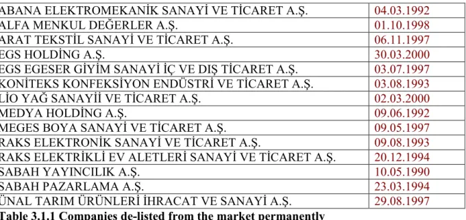
19 into account the financial conditions of the companies which are subject to pairs trading as well instead of just focusing statistical relationships of the historical price series. There were some companies in IMKB which used to exist in the past but no longer exist.
ABANA ELEKTROMEKANĐK SANAYĐ VE TĐCARET A.Ş. 04.03.1992
ALFA MENKUL DEĞERLER A.Ş. 01.10.1998
ARAT TEKSTĐL SANAYĐ VE TĐCARET A.Ş. 06.11.1997
EGS HOLDĐNG A.Ş. 30.03.2000
EGS EGESER GĐYĐM SANAYĐ ĐÇ VE DIŞ TĐCARET A.Ş. 03.07.1997 KONĐTEKS KONFEKSĐYON ENDÜSTRĐ VE TĐCARET A.Ş. 03.08.1993
LĐO YAĞ SANAYĐĐ VE TĐCARET A.Ş. 02.03.2000
MEDYA HOLDĐNG A.Ş. 09.06.1992
MEGES BOYA SANAYĐ VE TĐCARET A.Ş. 09.05.1997
RAKS ELEKTRONĐK SANAYĐ VE TĐCARET A.Ş. 09.08.1993
RAKS ELEKTRĐKLĐ EV ALETLERĐ SANAYĐ VE TĐCARET A.Ş. 20.12.1994
SABAH YAYINCILIK A.Ş. 10.05.1990
SABAH PAZARLAMA A.Ş. 23.03.1994
ÜNAL TARIM ÜRÜNLERĐ ĐHRACAT VE SANAYĐ A.Ş. 29.08.1997
Table 3.1.1 Companies de-listed from the market permanently Source: http://www.imkb.gov.tr/imkbweb/Home.aspx
So, in this research, instead of just focusing on the pure statistical relationship between the historical price series of the stocks, current financial conditions of the companies are considered as well. There are different criteria to measure of the healthiness of the current financial conditions of a company. One of these criteria is to look at how much profit the company makes. However, evaluating companies according to their profitability might be misleading. For example, a company which is suffering from severe financial problems can temporarily make a positive profit in an accounting period by selling its properties and providing hot money. There used to be firms in XU100, which made profit for just one period, and the next period losses of these companies were even larger.
20 Another problem with measuring the profitability of the companies is that a firm can make a loss in an accounting period because it spends a lot of money to make huge investments. Positive outcomes of these investments may appear in the future accounting periods instead of the current one. A company which makes loss due to its investments can make huge profits in the future accounting periods. So, looking profitable is not a good idea to check the healthiness of financial conditions of a company since measuring profit is complicated and misleading. A man who has just sold his car can carry large amount of cash for a period of time, but that does not necessarily mean that he is performing well in his financial world. The money came from selling a property, a car for example. Namely, somebody who has just bought a new house may experience a shortage of cash for some period of time, but in the future he can enjoy positive consequences of buying a house. Companies are alike too.
In my research, I used companies’ owners’ equities instead of profits to determine financial performance of the firms. If a company makes profit, the owner’s equity of the company gets larger. If a company makes a loss, owner’s equity of the company gets smaller, so, owner’s equity takes into account the profits but also a company’s owner’s equity can get larger when it spends its cash to make new investments. Therefore, owner’s equity is a better measurement criterion to measure financial healthiness of a company since it both takes into account the profit and the money spent on investments. In the table at the appendix 8.1, companies are listed according their owners’ equities amounts
In his pair trading strategy, Herlemont et al. (2004) had some pair formation constraints such as investing in stocks operating in the same sector. In this study, we have used the same constraint as well. Some researchers argued that stocks subject to pair trading can be chosen from different sectors as long as there is a strong long run correlation between
21 the historical price series of the stocks. Two stocks may have a close comovement relationship for a period of time; however, this relationship can break down permanently by some sector specific news. So, actually, investing in stocks operating in the same sector is a kind of risk control. By choosing the stocks from the same sector, we try to prevent a breakdown of the statistical relationship due to some sector specific news. In IMKB, there are three main sectors and each of these sectors is consisting of some subsectors.
CODE INDICE SUB-SECTOR INDICES
XUSIN
ISE NATIONAL INDUSTRIALS
FOOD, BEVERAGE, TEXTILE, LEATHER, WOOD, PAPER, CHEMICAL, BASIC METAL, MACHINERY XUMAL
ISE NATIONAL FINANCIALS
BANKS, INSURANCE, LEASING, FACTORING, HOLDING AND INVESTMENT
XUHIZ
ISE NATIONAL SERVICES
ELECTRICITY, TRANSPORTATION, TOURISM, WHOLESALE, TELECOMMUNICATIONS, SPORT Table 3.1.2 Sub-sector indices in XU100
As a result, this study has two risk controls on pair formation process. First, companies with the highest owners’ equities are chosen as pairs to make sure that companies whose stocks are subject to pairs trading are financially healthy. Secondly, companies are chosen from the same sector to slip away the effects of sector specific news.
22 3.2 TRADING RULES
Pair trading is implemented by determining the long run relationships between the historical price series of two financial assets, and taking the advantage of the short run deviations from this relationship. Here the emphasis is on this definition is short deviations. Many researches agreed on that as the two stocks have a close comovement relationship and this relationship does not break down permanently during the trading period, the strategy with the chosen pairs gives high rates of return. A researcher who is conducting his research currently has the all information about the past price series of financial assets. This researcher may set up a methodology which fits the past data perfectly; however, a methodology is good enough only if it continues its high performance as the new data keeps on coming. So, at that point there is another crucial question: When there is a significant deviation in the long run relationships of the prices of the stocks during the trading period, how does anyone understand the distinction between whether this deviation is a temporary short run deviation or a permanent long run breakdown of the long run correlation?
Unfortunately this distinction is not explained at all in the any of the past researches. Instead, it is mentioned as one of the potential risks which must be taken into account by investors who are already willing to make investment on such a risky field as stock exchange market. Here, we need to develop a method to understand when there is a significant deviation from the long run correlation whether this deviation is a temporary short run deviation which eventually disappears or a permanent long run breakdown of the long run correlation which causes the strategy end with a loss. In my research an indicator called DI+/DI- will be used to understand the distinction between those two.
23 3.2.1 Directional Movement Index (DI+/DI-)
DMI filtrates on price exchange rates lays in the basis and lets enter the market only if substantial trends exist. It is developed for increasing the strength of all upward or downward trends in the stock markets. The Directional Movement Index consists of Average Directional Index, or ADX, which defines the strength of the trend and DI+ and DI- which demonstrate the strength of the decreasing and increasing prices correspondingly. ADX is a moving average of Directional Index, or DX, with a smoothing constant makes time period selected for calculating upward and downward fluctuations twice as long.
Parameters:
1. N - the period of averaging
Calculation:
1. Calculation of the positive and negative directional movement - DM - +DMj and-DMj
if Highj> Highj-1, +DMj = Highj - Highj-1, differently +DMj = 0
if Lowj < Lowj-1, -DMj = Lowj-1 - Lowj, differently-DMj = 0
Smaller value from +DMj and -DMj is equated to zero. If they are equal, both are equated to
zero.
2. Calculation of the true range- TRj
TRj = max (|Lowj - Closej-1 |, |Highj - Closej-1 |, |Highj - Lowj |)
3. Calculation of a positive directional index and the negative directional index - +DIj and
24 If TRj = 0, +SDIj = 0, -SDIj = 0,
if TRj 0, +SDIj = +DMj / TRj; -SDIj =-DMj / TRj
Smoothing +SDI and -SDI by exponentional moving average (EMAve), we receive +DIj and -DIj
+DIj = EMAvej (+SDI, N)
-DIj = EMAvej (-SDI, N)
4. Calculation of the directional movement - DXj:
DXj = (| +DIj --DIj | / | +DIj +-DIj |)
In a trading system with DMI in the centre, there is a purchase signal when the DI+ value overcomes the DI-, and for a sell signal, search the point in which DI exceeds DI+. Both trading signals are given only if there is a rather strong trend. For instance, when the DI+ rises above DI- it is a clear purchase signal. In pairs trading, we trade two stocks simultaneously. Whenever we sell one stock, we buy the other one. So, we need a technical indicator which can give us information about the prices of the both stocks at the same time. Namely, we need to know the price movements of the stock we have in hand and also we need to know the price movements of the stock which we follow but do not have for the moment. The indicator DI+/DI- has two components, which are DI+ and DI-. DI+ gives us information about the price movements of the stock we have in hand, and DI- gives us information about the price movements of the stocks we follow. That is why we chose the indicator DI+/DI- as the ruling indicator, but not any other indicators. When we check the DI+/DI- we are able to check the price movements of the both stocks simultaneously.
25 3.2.2. Choosing Initial Pairs
First of all, two companies are chosen from the each sector. Namely, two companies from XUSIN, two other companies from XUMAL, and finally two other companies from XUHIZ are chosen. As it is mentioned before, in this study, owner’s equity is used to choose appropriate pairs. Therefore, for each sector, the first two companies with the largest owner’s equity are chosen. The table below summarizes the companies with the greatest owners’ equities in each year for each sector.
SUBSECTOR INDICES COMPANY CHOSEN OWNER'S EQUITY COMPANY RESERVED OWNER'S EQUITY
XUSIN EREGL 4,801,000,000 TL TUPRS 3,252,500,000 TL
XUHIZ TTKOM 7,690,000,000 TL TCELL 4,771,000,000 TL
XUMAL ISCTR 9,677,000,000 TL SAHOL 6,799,000,000 TL
Table 3.2.2.1 First two companies with the highest owners’ equities from each sector in 2005
SUBSECTOR INDICES COMPANY CHOSEN OWNER'S EQUITY COMPANY RESERVED OWNER'S EQUITY
XUSIN EREGL 5,399,000,000 TL TUPRS 3,461,000,000 TL
XUHIZ TTKOM 6,410,000,000 TL TCELL 5,557,000,000 TL
XUMAL ISCTR 9,410,000,000 TL AKBNK 7,065,000,000 TL
Table 3.2.2.2 First two companies with the highest owners’ equities from each sector in 2006
SUBSECTOR INDICES COMPANY CHOSEN OWNER'S EQUITY COMPANY RESERVED OWNER'S EQUITY
XUSIN EREGL 6,004,000,000 TL TUPRS 4,111,000,000 TL
XUHIZ TCELL 6,670,000,000 TL TTKOM 6,122,000,000 TL
XUMAL ISCTR 10,603,000,000 TL AKBNK 10,600,000,000TL
Table 3.2.2.3 First two companies with the highest owners’ equities from each sector in 2007
SUBSECTOR INDICES COMPANY CHOSEN OWNER'S EQUITY COMPANY RESERVED OWNER'S EQUITY
XUSIN EREGL 5,936,000,000 TL ENKAI 4,961,000,000 TL
XUHIZ TCELL 8,084,000,000 TL TTKOM 5,113,000,000 TL
XUMAL AKBNK 11,208,000,000 TL KCHOL 9,750,000,000 TL
26 3.2.3. Trades for XUSIN Indices
For example, as long as XUSIN is concerned, according to data in 31.12.2005, EREGL has the greatest owner’s equity with 4,801,000,000 TL among all companies belonged to XUSIN indices and TUPRS has the second greatest owner’s equity according to data in 31.12.2005. (table 3.2.2.1)
EREGL, as having the largest owner’s equity is called “the chosen stock” whereas TUPRS, as having the second largest owner’s equity is called “reserved stock”. First day of the trading period is 01.01.2006. At the beginning of the market opening, we buy the “chosen stock”, namely EREGL in this case since it has the greatest owner’s equity. After that time, we pay attention only to EREGL and TUPRS. When a new signal comes from our indicator DI+/DI- we will change the pair, we will sell EREGL and buy TUPRS. As long as DI+ is greater than DI-, the indicator tells us to keep the chosen stock we have. When DI- rises above DI+, we will sell the chosen stock (EREGL) and buy the reserved stock (TUPRS). The table below shows the summary of trades.
DATE DI+ DI- SIGNAL PRICE SIGNAL PRICE RETURN
100 TL BECOMES 03.02.2006 22,04 21,3 BUY EREGL 3,36
17.04.2006 17,76 28,31 SELL EREGL 3,17 BUY TUPRS 16,71 -5,65% 94,35 11.09.2006 22,72 19,95 BUY EREGL 2,9 SELL TUPRS 18,82 12,63% 106,26 24.12.2007 18,23 19,06 SELL EREGL 7,2 BUY TUPRS 24,97 148,28% 263,83 03.03.2008 18,68 16,49 BUY EREGL 6,16 SELL TUPRS 23,46 -6,04% 247,9 01.09.2008 22,5 22,7 SELL EREGL 7,75 BUY TUPRS 23,89 25,81% 311,86 17.11.2008 23,78 17,21 BUY EREGL 4,06 SELL TUPRS 13,17 -44,87% 171,94 02.03.2009 18,48 21,73 SELL EREGL 3,48 BUY ENKAI 4,1 -14,29% 130,35 22.06.2009 20,38 19,96 BUY EREGL 4,4 SELL ENKAI 4,74 15,61% 150,7 Table 3.2.3.1 Return table of the trades for XUSIN.
In 17.04.2006 for the first time, DI - gets greater than DI+, as long as this happens during the trading day, we immediately sell EREGL at its current price and we buy TUPRS
27 instead. We keep TUPRS as long as DI- is greater than DI+. In 11.09.2006, DI+ rises above DI- again, which is a signal to sell TUPRS and buy the EREGL back. In 24.12.2007 DI- gets greater than DI+ again, which is a signal to sell EREGL and buy TUPRS back. As it is understood, whenever DI+ gets greater than DI- we buy the “chosen stock” back and keep it as long as DI+ is greater than DI-. If anytime DI- gets greater than DI+ we sell the “chosen stock” and buy the reserved stock back. This process continues unless one of the “chosen stock” and “reserved stock” changes. Note that we call the stock with the highest owner’s equity as the “chosen stock” and the stock with the second highest owner’s equity is called as “reserved stock”.
So according data in 31.12.2008, EREGL has still the highest owner’s equity but now ENKAI instead of TUPRS had the second highest owner’s equity. Therefore “chosen stock” is still EREGL but, the reserved stock changed from TUPRS to ENKAI. After this time pair trading will be taking place between EREGL and ENKAI. That means the portfolio is not a static portfolio but a dynamic one. At the end of each year, current values of owner’s equity are announced and if there is difference in the order of the companies the methodology takes this into account also. For example, between 2005 and 2007 EREGL and TUPRS are the first two companies with the highest owners’ equities, therefore, pair trading is taking place between these two companies, however, in 2008 EREGL and ENKAI are the first two companies with the highest owners’ equities (table 3.2.2.4.), therefore, pair trading is taking place between these two companies now.
28 3.2.4. Trades for XUMAL Indices
As long as XUMAL is concerned, according to data in 31.12.2005, ISCTR has the greatest owner’s equity with 9,677,000,000 TL among all companies belonged to XUSIN indices and SAHOL has the second greatest owner’s equity with 6,799,000,000 TL according to data in 31.12.2005. (table 3.2.2.1)
ISCTR, as having the largest owner’s equity is called “the chosen stock” whereas SAHOL, as having the second largest owner’s equity is called “reserved stock”. First day of the trading period is 01.01.2006. At the beginning of the market opening, we spent all our money to buy the “chosen stock”, namely ISCTR in this case. After that time, we pay attention only to ISCTR and SAHOL. When a new signal comes from our indicator DI+/DI- we will change the pair, we will sell ISCTR and buy SAHOL. As long as DI+ is greater than DI-, the indicator tells us to keep the chosen stock. Once, DI- becomes greater than DI+ we will sell the chosen stock (ISCTR) and buy the reserved stock (SAHOL). The table below shows the summary of trades.
DATE DI+ DI- SIGNAL PRICE SIGNAL PRICE RETURN
100 TL BECOMES 02.01.2006 BUY ISCTR 6,73
23.01.2006 17,59 18,25 SELL ISCTR 7,37 BUY SAHOL 5,28 9,5% 109,5 15.05.2006 21,29 15,33 BUY ISCTR 5,83 SELL SAHOL 4,98 -5,68% 103,28 30.04.2007 17,33 18,77 SELL ISCTR 5,77 BUY AKBNK 7,10 -1,02% 102,23 01.10.2007 20,14 17,06 BUY ISCTR 5,94 SELL AKBNK 8,70 22,53% 125,26 23.06.2008 18,08 25,63 SELL ISCTR 4,14 BUY AKBNK 4,62 -30,3% 87,31 18.08.2009 16,38 19,79 BUY KCHOL 3,50 SELL AKBNK 7,95 72,07% 150,23 Table 3.2.4.1 Return table of the trades for XUMAL
29 3.3 RETURN CALCULATION
In table above, we have returns as percentage and a cumulative return which shows how a portfolio of 100 TL changed up to now. To calculate the returns as percentage the following formula is used.
Percentage Return = (Ps-Pb)/Pb where;
Ps: Current market price of the stock when it is sold
Pb: Current market price of the stock when it is bought
For example, at 03.03.2008 we bought EREGL at a price of 6,16. This price is Pb. And at 01.09.2008 we sold EREGL at a price of 7,75. This price is Ps. So,
Percentage Return = (Ps-Pb)/Pb = (7,75-6,16)/6,16 =0,2581 or 25,81%
3.4 PAIR TRADING WITH MARKET CONSIDERATIONS
In most studies, pair trading is considered as a market neutral strategy. Namely, traders do not bet on the direction of the market. However, current economic conditions of a country have great effects on the stock exchange market. For example, in the past when there was an economic crisis in 1999, values of all stocks (without any exception) decreased. So, if somehow we can determine these long break downs, we may prevent our portfolio from losses. For example, in this study, we applied pairs trading strategy between EREGL and TUPRS and later between EREGL and ENKAI between 2006 and 2009, as a result, 100 TL became 150,7 TL in three years. However, there were some transactions at which percentage returns were negative. For example, 01.09.2008 and 17.11.2008, our portfolio made a 44,87% loss. If we take into account the market conditions, performance of the strategy may increase.
30 So, before investing in any stock, we first set up an alert system which continuously tells us whether the current economic climate is appropriate to make investment or not. If current economic climate is not appropriate, we sell all the stocks we have immediately and hold cash until a signal which tells us that current economic climate is appropriate to make investment again. We will run the same pairs trading example once more but this time an alert system about IMKB is used as well.
The alert system is simple. We again use the indicator DI+/DI- because of the reasons I mentioned above to check whether current economic climate is appropriate or not. If DI+ is greater than DI-, that means we are allowed to make investments, if DI- is greater than DI+, we will sell all the stocks immediately and begin to hold cash until DI+ becomes greater than DI- again. The table below summarizes the appropriate periods to make investment in stocks.
DATE DI+ DI- SIGNAL UNTIL DURATION
20.06.2005 20,2 18,52 ENTER 15.05.2006 330 15.05.2006 21,48 28,89 OUT 16.10.2006 152 16.10.2006 24,3 22,06 ENTER 19.11.2007 398 19.11.2007 24,87 26,08 OUT 06.04.2009 138 06.04.2009 24,87 23,75 ENTER CURRENT DAY 140 Table 3.4.1 Signals for IMKB IN and IMKB OUT generated by DI+/DI-
For example, we began pairs trading by buying EREGL at the beginning of the trade period. At 15.05.2006 DI- becomes greater than DI+, which means an IMKB out signal. Therefore, as soon as we see this signal during the trading period, we sell our current stocks and begin to hold cash until 16.10.2006. At 16.10.2006, an IMKB enter signal is generated by the DI+/DI- indicator. At 16.10.2006, DI+ becomes greater than DI- again after 152 days later. So, we will spend our current cash to by the chosen stock (the one with the highest owner’s equity) again. The only difference is there is an on/off alert system here which means
31 we do not have a stock all the time. In classical pairs trading, traders hold stock every moment of every day. Whenever they sell a stock, they buy the other one back. However, in this study, we may hold the “chosen stock” or we may hold the “reserved stock” or we may not have any stocks at all for some period of time. The table below summarizes a market behavioral pairs trading strategy.
DATE DI+ DI- SIGNAL PRICE SIGNAL PRICE RETURN
100 TL BECOMES 03.02.2006 22,04 21,3 BUY EREGL 3,36
17.04.2006 17,76 28,31 SELL EREGL 3,17 BUY TUPRS 16,71 -5,65% 94,35 15.05.2006 OUT OUT OUT 2,85 OUT 17,52 4,85% 98,92
16.10.2006 IN IN IN IN
16.10.2006 37,176 15,76 BUY EREGL 3 16,88
19.11.2007 OUT OUT OUT 7,48 OUT 23,65 149,30% 246,62
06.04.2009 IN IN IN IN
06.04.2009 26,22 31,99 3,3 BUY ENKAI 4,08
04.05.2009 18,213 16,443 BUY EREGL 3,94 SELL ENKAI 4,68 14,70% 282,88 Table 3.4.2 Pairs trading as a market behavioral strategy
At 17.04.2006 DI- becomes greater than DI+ therefore, we sell EREGL and buy TUPRS with the all money. At 15.05.2006 an IMKB out signal is generated by DI+/DI- (check table 3.4.1), so we sell TUPRS but by nothing, instead we hold cash until a IMKB IN signal is generated by DI+/DI-. At 16.10.2006 an IMKB IN signal is generated, so we spend all our cash and invest in EREGL. At 16.10.2006 we invested in EREGL not TUPRS because at that date DI+ is greater than DI-. We keep EREGL until 19.11.2007 since a new IMKB OUT signal is generated (check table 3.4.1). so, we sell all the stocks and begin to hold cash again. At 06.04.2009 A new IMKB IN signal is generated by DI+/DI- (check table 3.4.1). Therefore we spend all our cash and make an investment in ENKAI stocks. At 06.04.2009 we invested in ENKAI stock but not EREGL since at that date DI- is greater than DI+.
32 As a result, by allowing an alert system for IMKB IN/IMKB OUT performance of the strategy increased significantly.
33
4. CONCLUSION
Pair trading is used as a market strategy by many researchers and academicians and even by some hedge funds up to now. Almost each of them used his own version of pairs trading strategy. In this study a market behavioral (market friendly) pairs trading strategy is used to examine the empirical results in IMKB. In this paper there were some risk controls to improve the performance of the strategy. Some restrictions were imposed while choosing the appropriate stocks for pair trading.
First of all, we were only interested in stocks whose companies are financially doing well. In order to understand the current financial conditions of the companies we used their current owners’ equities. Secondly, the pairs are formed by the stocks which are operating in the same sector. By choosing stocks from the same sector, we aimed that sector specific information would make both stocks affect so; the relative value of the pair would remain unchanged. Thirdly, unlike the classical pairs trading strategies, we did not carry positions on the stocks all the time; instead, there were some periods of times that we only held cash but nothing else. Sometimes we held positions on the stocks, sometimes we held only cash. When economic climate was not appropriate, we chose to wait in cash. Finally, our model was not a static model but a dynamic one. At the end of each year current values of owners’ equities of the companies are updated. So, if there is a change in the order of the owners’ equities, we change the stocks accordingly. The table 8.1 shows how owner’s equities of the companies changed each year.
As a result, by using this market friendly, dynamic pairs trading technique, we were able to achieve quite good results. Studies about the pairs trading are limited and most of them are done by examining the stock exchange markets of the developed countries. More and
34 more researchers are getting interested in pairs trading in each day. So, in the future there may be more pairs trading studies on the stocks of the emerging markets such as IMKB as well. Finally, even though, the return results were significantly good in this dynamic, market friendly pairs trading strategy, investors should keep in mind that making investment on a stock exchange market carries some risks and it is not possible to build a totally risk-free strategy.
35
5. REFERENCES
Cetkin, Umit. (2008), Pairs Trading: Building Trading Strategies for Asset Pairs Price Dynamics, Master Thesis, Istanbul Bilgi University
Do, B. & Faff, R. & Hamza, K. (2006), A New Approach to Modeling and Estimation for Pairs Trading, Working Paper, Monash University.
Ehrman, Douglas S. (2006), The Handbook of Pairs Trading: Strategies Using Equities, Options, and Futures, John Wiley & Sons, New Jersey, pages 19-20.
Engle, Robert F. & Granger, Clive W.J. (1987), Cointegration and Error Correction: Representation, Estimations and Testing, Econometrica, Volume 55, pages 251-267
Gatev, E. & Goetzmann, W.N. & Rouwenhorst, K.G. (2006), Pairs Trading: Performance of a Relative-Value Arbitrage Rule, Working Paper, Yale School of Management.
Granger, Clive W.J. (1981), Some properties of time series data and their use in econometric model specification, Journal of Econometrics, Volume 16, pages 121-130.
Herlemont, D. (2004), Pairs trading, convergence trading, cointegration, YATS Finances & Tecnologies
Hogan, S. & Jarrow, R. & Teo, M. & Warackha, M. (2003). Testing market efficiency: Using Statistical Arbitrage with Applications to Momentum and Value Strategies.
Holton, Glyn A. (2003), Negatively Skewed Trading Strategies, Derivatives Week, Volume 12, pages 8-11
Huck, N. (2008), Pairs Selection and Outranking: An application to the S&P 100 Index, European Journal of Operational Research
36 Jagedeesh, N. & Titman, S. (1993). Returns to Buying Winners and Selling Losers: Implications for Stock Market Efficiency, The Journal of Finance, Volume 48, No:1, pages 65-86.
Larsson, E. & Larsson, L. & Aberg, W. (2003), What Happened to the Quants in August 2007? Journal of Investment Management, Volume 5, NO:4
Nath, P. (2003). High frequency Pairs Trading: Risk and Rewards for Hedge Funds, Working paper, London Business School.
Ozkaynak, Ozkan. (2007), Statistical Arbitrage: A Study in Turkish Equity Market, Master Thesis, Istanbul Bilgi University.
Perlin, Marcelo S. (2007), Evaluation of Pairs Trading Strategy at the Brazilian Financial Market , Working Paper, ICMA, Reading University
Perlin, Marcelo S. (2007), M of a kind, A multivariate Approach at Pairs Trading, available at, SSRN:http://ssrn.com/abstract=952782
Suslava, O. & Sudak, D. (2003), Behavioral Statistical Arbitrage, Program in Banking and Finance, University of Lausanne.
Vidyamurthy, G.(2004). Pairs Trading, Quantitative Methods and Analysis, John Wiley & Sons, New Jersey
http://en.wikipedia.org/wiki/Pairs_trade
http://www.imkb.gov.tr/imkbweb/Home.aspx
http://www.forexrealm.com/technical-analysis/technical-indicators/directional-movement-index.html
37
6. APPENDIX
Owners’ Equities of the Companies in IMKB (TL) (from smallest to largest)
Hisse 2005/12 2006/12 2007/12 2008/12 DARDL E -191.165.802 -243.600.503 -207.831.898 -286.672.449 ZOREN E 311.408.675 285.779.429 273.380.013 -81.820.907 CBSBO E -35.037.760 -47.535.458 -47.633.756 -72.294.787 MZHLD E -11.187.547 -19.187.474 -20.959.190 -31.721.617 KERVT E -15.821.880 -24.127.041 -11.354.044 -28.529.775 TRNSK E 23.018.118 23.226.958 10.771.811 -28.426.300 EPLAS E 694.407 -8.834.956 -8.226.226 -27.374.725 BERDN E 4.072.244 -15.773.466 -23.048.676 -24.854.266 MAKTK E 22.884.187 20.313.985 -63.695.897 -21.748.645 EMKEL E 922.141 -1.968.316 -1.991.451 -1.579.225 ISATR E 4.915 3.414 3.847 3.428 ISBTR E 142.535 98.997 111.555 99.406 TKSYO E - 2.291.255 1.977.911 1.075.218 METYO E - 2.543.633 2.926.859 1.313.213 CEYLN E 7.002.303 7.533.513 8.295.885 1.903.617 EVNYO E 3.423.644 3.386.402 3.435.134 2.027.993 MERKO E 16.118.307 15.721.262 12.019.274 2.081.220 BISAS E 13.278.073 2.164.254 1.791.793 2.464.424 MRTGG E 8.860.745 7.678.367 6.422.539 2.678.964 MYZYO E 3.464.796 5.527.937 6.455.342 2.730.791 MZBYO E - 3.148.053 2.866.611 2.784.980 AVRSY E 7.139.913 5.396.031 6.564.688 2.859.277 HDFYO E 3.034.522 3.336.401 3.594.199 3.091.373 INFYO E 3.509.059 4.098.345 4.408.650 3.091.434 ESEMS E 3.977.130 -1.150.758 8.255.324 3.121.606 ATLAS E 4.447.689 5.353.361 7.616.309 3.165.527 ATSYO E 6.511.748 9.531.497 11.721.088 3.553.758 DURDO E 8.884.326 10.201.718 6.848.395 3.688.482 MRBYO E - 3.091.260 3.627.421 3.795.682 TCRYO E - 4.949.966 5.048.924 3.865.119 VKFRS E 10.652.862 4.233.797 4.174.825 4.502.652 FRIGO E 10.817.391 10.153.340 8.901.965 4.509.720 METUR E 13.689.815 13.385.066 12.433.338 4.715.946 BSKYO E - 2.712.373 4.996.693 4.717.776 BURVA E 8.036.301 7.676.374 5.979.840 4.931.480 BJKAS E 37.145.901 18.945.338 22.634.782 5.090.355 IBTYO E 5.597.952 4.968.907 5.526.152 5.290.564
38 ETYAT E - - 5.168.898 5.426.332 BUMYO E 3.639.825 6.066.442 6.750.082 5.581.038 GDKYO E 3.227.160 5.500.868 8.465.693 5.941.977 LINK E 9.131.133 8.031.048 6.314.472 6.548.638 BROVA E 11.524.479 9.637.415 7.711.083 6.686.566 ATAYO E 3.784.016 3.999.526 9.515.246 7.181.123 SELGD E 17.126.819 21.191.958 11.897.605 7.297.507 VKING E 35.262.738 23.667.857 23.978.150 7.317.326 BURCE E 9.098.002 8.067.478 7.441.244 7.490.601 TACYO E 9.204.063 9.854.128 12.232.243 7.920.439 MTEKS E 15.943.827 10.386.119 13.926.198 8.099.218 SERVE E 7.364.434 8.182.969 9.339.777 8.136.337 OYAYO E - 10.230.198 10.958.614 8.343.995 INTEM E 28.016.471 22.923.406 24.301.379 9.197.293 VARYO E 4.499.105 4.874.914 8.659.798 9.387.031 EMNIS E 17.997.828 17.360.370 16.442.749 9.508.568 EGCYO E 11.789.706 7.914.961 19.832.823 9.606.998 EMBYO E - 3.077.994 10.012.670 10.021.523 BFREN E 22.222.882 22.541.424 23.666.476 10.143.537 YTFYO E 7.395.696 12.270.203 14.359.738 10.648.045 LUKSK E 12.247.252 13.099.896 12.219.230 11.035.954 DOGUB E 21.639.788 8.865.683 7.602.978 11.080.516 VKFYT E 11.644.185 11.875.817 14.103.333 11.547.073 OZGYO E 5.412.437 6.123.323 9.138.696 11.729.307 IDAS E 35.702.943 33.232.839 32.955.093 11.821.669 ALYAG E 10.031.547 11.979.574 11.705.876 11.990.617 AFMAS E 23.213.271 21.046.488 21.173.980 12.157.341 DERIM E 7.554.668 10.324.511 12.390.818 12.247.906 HZNDR E 9.923.266 12.790.279 13.727.386 12.772.475 OKANT E 10.206.536 8.904.331 8.415.676 13.074.592 PKENT E 17.739.713 13.796.574 10.359.110 13.105.553 SKPLC E 20.491.468 21.056.499 38.042.544 14.039.225 TIRE E 82.542.977 82.397.255 79.360.596 14.727.349 KNFRT E 9.228.985 11.496.124 17.793.992 15.499.238 SEKFK E -3.771.566 -6.038.124 7.819.963 15.819.481 FNSYO E 23.430.975 24.730.857 28.197.301 16.390.844 KLBMO E -15.892.930 -4.989.866 15.519.334 16.795.313 DGATE E 5.696.210 13.898.085 16.845.566 17.107.889 GEREL E 12.396.798 14.073.856 14.639.533 17.188.299 TSKYO E 17.671.867 20.017.652 22.149.149 18.167.716 GRNYO E 9.139.060 18.904.054 24.049.149 20.021.305 ESCOM E 20.868.197 21.079.314 21.316.757 20.293.844 ERSU E 23.272.034 20.708.327 20.851.964 20.687.057 USAK E 23.533.652 21.833.766 23.172.650 21.148.845
39 ARMDA E 10.295.000 19.750.000 19.078.310 21.897.047 ECBYO E 22.301.461 21.036.361 27.064.781 22.032.032 AKIPD E 69.749.524 53.930.218 45.949.464 22.740.846 GEDIZ E 9.877.823 8.412.586 25.765.375 23.339.670 YYGYO E 31.385.014 27.744.662 26.304.509 24.153.895 PKART E 22.954.916 21.954.995 22.466.337 24.191.130 PRTAS E 26.362.823 22.477.200 23.565.606 24.472.568 DENCM E 28.161.784 28.938.129 27.141.361 25.317.615 KLMSN E 26.069.269 31.890.171 32.654.762 26.027.542 DITAS E 26.894.299 27.640.454 27.111.493 26.138.918 ARFYO E 20.219.852 30.690.602 37.480.031 28.549.498 TUKAS E 67.073.778 55.637.249 43.299.819 28.809.751 KAPLM E 29.862.787 32.045.859 32.512.538 31.137.924 FMIZP E 17.768.899 22.374.052 19.147.210 31.610.694 SILVR E 12.210.120 33.762.636 32.306.193 31.670.041 CMBTN E 32.433.646 35.231.438 37.667.084 31.823.711 FVORI E 79.187.031 60.717.307 68.029.073 32.074.457 MIPAZ E 21.505.796 23.582.751 20.473.756 32.168.927 AKSUE E 25.285.602 25.798.511 26.178.234 32.276.416 TEKTU E 38.056.700 35.729.467 33.712.369 32.335.995 CELHA E 25.673.019 28.201.942 28.815.011 34.173.767 EDIP E 69.948.014 55.969.757 53.159.916 34.325.472 BRMEN E 47.319.742 49.986.463 50.934.206 35.132.785 LOGO E 33.301.349 30.170.933 37.396.296 36.205.293 KRSTL E 38.948.769 38.712.646 38.889.476 36.437.828 PENGD E 35.466.785 20.783.960 28.088.040 37.015.527 VAKFN E 29.724.000 36.367.000 32.985.000 37.240.000 AKYO E 48.859.654 50.419.234 51.971.879 37.809.322 TEKFK E 23.726.281 27.745.363 32.008.171 38.750.591 DOBUR E 34.165.926 34.492.546 39.760.140 38.983.562 EGEEN E 28.771.593 38.013.474 36.537.888 39.481.413 DNZYO E 25.138.915 36.322.208 46.827.540 40.148.271 MAALT E 51.659.015 45.212.297 41.397.405 40.306.599 GARFA E 24.025.173 28.622.110 34.346.135 41.427.917 ARENA E 26.381.019 33.650.375 34.442.115 42.555.510 FENIS E 29.711.845 33.510.765 36.466.061 43.415.960 CRDFA E 27.391.933 29.028.830 35.755.999 45.512.674 ALCTL E 24.119.797 31.493.694 30.533.968 45.610.784 ERBOS E 26.197.020 36.458.307 45.448.345 45.954.078 MEMSA E 15.005.380 87.601.254 68.986.834 45.999.319 DYOBY E 49.519.426 38.814.343 80.365.746 48.829.110 ADEL E 29.622.720 36.243.952 39.916.725 49.407.278 YUNSA E 69.706.590 75.276.826 72.451.087 50.024.929 SAGYO E -24.630 7.115.158 58.952.984 50.299.085
40 YATAS E 47.013.799 51.343.383 54.807.802 51.266.486 BOYNR E -1.821.398 37.208.897 51.248.765 51.404.871 VANET E 24.841.896 24.628.465 24.417.751 52.504.908 BAKAB E 39.369.546 48.790.484 51.401.895 53.479.721 NUGYO E 37.062.115 40.903.010 47.473.879 53.535.544 YKRYO E 44.079.245 48.296.706 60.001.543 53.878.386 AFYON E 34.557.888 44.755.833 53.638.156 54.989.869 DENTA E 69.931.756 80.367.577 88.620.775 55.144.057 SONME E 89.369.247 78.583.399 69.083.476 55.381.239 NTTUR E 55.548.883 53.734.124 145.025.960 56.233.154 CYTAS E 39.300.072 53.092.122 52.865.665 60.906.463 ANELT E 54.557.618 52.384.791 64.239.682 61.147.970 PINSU E 39.611.558 48.842.044 56.426.200 61.326.279 DESA E 63.207.242 59.662.177 65.610.842 62.214.816 RAYSG E 21.909.315 16.195.692 49.079.916 62.244.087 KARSN E 57.842.645 46.885.877 108.198.544 64.812.240 PIMAS E 23.299.552 31.878.480 69.748.582 66.435.273 DMSAS E 68.495.178 70.397.825 69.915.100 70.498.906 VKGYO E 52.981.880 57.504.072 62.701.299 70.814.308 SNPAM E 95.443.280 90.983.886 102.778.543 72.119.885 KRTEK E 63.103.455 64.298.686 68.314.931 73.025.210 TBORG E 62.746.844 -1.058.068 10.774.749 78.554.567 AYCES E 68.637.318 63.886.538 74.715.998 78.752.351 UCAK E 82.841.796 152.172.442 56.929.050 79.031.577 HEKTS E 66.118.749 71.465.617 76.471.888 79.256.872 KAREL E 33.378.968 62.309.312 70.398.584 79.539.402 TSPOR E 35.774.555 42.512.529 70.429.570 81.768.064 ARSAN E 119.593.846 115.777.825 105.338.987 84.019.128 ISAMB E -3.322.369 20.404.876 32.498.341 85.306.093 BANVT E 83.638.116 96.925.873 152.449.322 85.811.277 KUTPO E 84.238.454 85.026.648 85.263.783 86.692.903 EGYO E 83.737.467 79.065.957 87.591.894 86.916.702 FENER E 65.590.727 73.294.513 72.682.053 87.576.012 EGPRO E 63.546.046 73.855.082 89.308.720 87.837.397 INDES E 61.486.266 73.878.261 86.221.286 88.088.902 PEGYO E 37.891.049 32.459.186 72.745.944 90.256.113 KRDMB E 34.495.894 44.909.656 53.473.293 90.290.946 MARTI E 89.031.508 93.041.615 90.251.958 91.145.400 IHEVA E 32.771.393 33.976.702 80.734.021 93.323.015 GENTS E 65.377.082 79.816.664 88.983.386 93.808.899 TUDDF E 175.947.357 192.389.991 120.500.687 97.457.522 ALKA E 84.952.888 82.827.499 89.062.018 97.887.616 YKGYO E 92.249.003 99.094.683 106.148.029 98.260.122 ATEKS E 125.558.690 125.096.489 118.303.073 101.253.018