Evaluation of Internal MRI Coils Using Ultimate
Intrinsic SNR
Haydar C
¸elik,
1Yigˇitcan Eryaman,
1Ayhan Altıntas¸,
1I.A. Abdel-Hafez,
1and
Ergin Atalar
1,2,3,4*
The upper bounds of the signal-to-noise ratio (also known as the “ultimate intrinsic signal-to-noise ratio” (UISNR)) for internal and external coils were calculated. In the calculation, the body was modeled as a dielectric cylinder with a small coaxial cylin-drical cavity in which internal coils could be placed. The calcu-lated UISNR values can be used as reference solutions to eval-uate the performance of internal MRI coils. As examples, we evaluated the performance of a loopless antenna and an en-dourethral coil design by comparing their ISNR with the UISNR. Magn Reson Med 52:640 – 649, 2004. © 2004 Wiley-Liss, Inc.
Key words: internal coils; external coils; endoluminal coils; UISNR; SNR in MRI; RF coils
In MRI, the performance of radiofrequency (RF) coils plays a critical role in determining the quality of acquired im-ages. Optimal RF coil designs differ for different imaging locations in the body. However, studies concerning opti-mal coil designs generally have been performed for a given coil geometry (1,2).
There are various types of disposable internal coils, such as opposed solenoids (3,4), expandable coils (5– 8), elon-gated loops (9), and loopless antennas (10), for use in various body cavities, including the vagina, esophagus (11), urethra (12), blood vessels (10,13), and rectum (14). Although the SNR of MRI images increases when these coils are used, it is not possible to directly compare the performance of the internal coils with that of the external coils. Furthermore, there is no formal method by which to evaluate the performance of these internal coil designs in terms of SNR. In a previous study (15), with a similar motivation, we calculated the value of the ultimate intrin-sic SNR (UISNR) for external coils. The ISNR was defined for a given sample-coil combination as the MR signal volt-age received from a unit volume of the sample divided by the root-mean-square (RMS) noise voltage received per square root of bandwidth (16). Since the UISNR is inde-pendent of coil design, the information obtained from the
UISNR value can be used as a reference to potentially improve the performance of a coil.
In this work we reformulated the calculation of the UISNR to extend it to internal MRI coils (17). We used the cylindrical body model for both UISNR values in order to utilize cylindrical symmetry, and coordinates to represent EM fields propagating inside the body. This idea brings simplicity, and does not affect the result negatively. This model has been used by other researchers (1,18,19), and the results obtained with this model are consistent with previous work. A cylindrical body model with uniform electromagnetic (EM) properties was used to approximate the human body (see Fig. 1). In this model, a coaxial cylindrical cavity is assumed to exist at the center of the body, simulating blood vessels or similar structures in which internal RF coils can be placed. With this structure, surface (or external) RF coils can be placed on the exterior surface of the body, while internal coils are placed in the central cavity.
To obtain the signal and noise voltages picked up by a receiving coil, one can use the reciprocity principle and determine the EM fields generated by the receiving coil when it is used as a transmitter (18). By assuming that body noise is dominant among other sources of noise, and with the constraint of having a fixed value of the transverse circularly polarized component of the magnetic field at the point of interest, one can maximize SNR by minimizing the total power deposited in the body (15). Therefore, for a given point of interest and EM property of the body, the optimum EM field distribution must be calculated. As shown below, this is not only a more general problem than the parametrical optimization of a given coil structure, it is also a much easier problem to solve.
The UISNR values for various frequencies and cavity sizes were calculated. The results were used to measure the performance of a loopless antenna (10) and an en-dourethral coil (12) in the cavity.
THEORY
To calculate the UISNR, we optimized the associated EM field rather than a specific coil geometry (15). The UISNR depends on the geometric and electrical properties of the body, and the position of the point of interest. We assumed a cylindrical body and the EM fields inside the human body to be expressed as a weighted sum of the cylindrical waves, which served as basis functions. To obtain the UISNR value, the noise level in the system should be considered. Power losses, such as conductor losses, radi-ation losses, and body losses, primarily determine the noise level. For a system with well-designed RF coils, conductor and radiation losses can be minimized, and the
1Department of Electrical and Electronics Engineering, Bilkent University, Ankara, Turkey.
2Departments of Radiology, Johns Hopkins University, Baltimore, Maryland. 3Department of Biomedical Engineering (BME), Johns Hopkins University, Baltimore, Maryland.
4Department of Electrical and Computer Engineering (ECE), Johns Hopkins University, Baltimore, Maryland.
Grant sponsor: NIH; Grant numbers: RO1RR15396; R01HL61672; R01HL57483.
*Correspondence to: Ergin Atalar, Ph.D., Department of Electrical and Elec-tronics Engineering, Bilkent University, 06800 Ankara, Turkey. E-mail: [email protected]
Received 11 December 2003; revised 7 May 2004; accepted 10 May 2004. DOI 10.1002/mrm.20200
Published online in Wiley InterScience (www.interscience.wiley.com).
body loss remains the main factor that limits the SNR value. The expression for the ISNR (15,16), which is inde-pendent of imaging parameters, is
⌿ ⫽
冑
2M0冑
4kbTRB⫹ [1]
where kb is the Boltzmann’s constant, T is the sample temperature, is the Larmour frequency, and M0is the instantaneous magnetic moment per sample voxel imme-diately after a 90° pulse is applied. B⫹is the right-hand circularly polarized magnetic field component, and is de-fined as B⫹⫽ H⫹, where is the magnetic permeability and H⫹⫽ (H⫺ jH)/公2 when the main magnetic field is along the⫹z direction and for a time convention of ejt (suppressed), where j is the complex number 公⫺1. Mag-netic permeability in the body is assumed to be uniform and equal to the permeability of free space,0. R is the real part of the input impedance seen by the input terminals of the coil. According to the reciprocity principle (18,20), one can find the value of R by calculating the total dissipated power when the receiver coil is used as a transmitter and driven by a 1 amp RMS current source from its input terminals.
As mentioned above, the body loss, Rbody, is the main factor in power dissipation and noise level. For a properly designed system R⬵ Rbody, and with a unit RMS current excitation, it becomes Rbody⫽ Ploss, where Ploss is power loss in the body. We assume that outside the body we have a lossless region; thus, there is no contribution to power dissipation from the fields in the outside region. Since we do not specify the fields outside the body, we do not need to impose boundary conditions.
In order to obtain maximum SNR, Rbodymust be mini-mized, while H⫹must be maximized. Since with the aid of a simple transformer, the value of H⫹ can be modified without affecting the SNR, in our calculations we arbi-trarily assumed that the right-hand circularly polarized magnetic field at the point of interest, rᠬ0, was fixed to one, i.e., H⫹(rᠬ0)⫽ 1. Therefore, the problem of calculating the UISNR reduces to a minimization of Rbody(15).
EM Field Expression for a Cylindrical Body
For an infinitely long cylindrical body, the EM fields can be written in terms of an inverse Fourier transform of
cylindrical wave function expansions (18). When one con-siders a cylindrical body of finite length, the Fourier inte-gral becomes the Fourier series at discrete spectral values. For the problem considered here, the optimum EM field that will minimize power dissipation inside the body can be written as the weighted sum of the cylindrical waves:
Eᠬ ⫽
冘
m⫽⫺⬁ ⬁冘
n⫽⫺⬁ ⬁ Eᠬmn, [2]where m and n are integer variables representing the Fou-rier modes (FouFou-rier components).
The cylindrical waves can be generated from the z-components of electric and magnetic field intensities, which are the solutions for scalar Helmholz equations:
Ezmn⫽ 共AmnJm共n兲 ⫹ CmnYm共n兲兲ejme⫺jznz [3]
Hzmn⫽ ⫺j共BmnJm共n兲 ⫹ DmnYm共n兲兲ejme⫺jznz, [4] where ⑀ is the electric permittivity, and Jm and Ym are
mth-order first and second kinds of Bessel functions,
re-spectively (the second kind of Bessel function is also called a Neumann function). In addition, Amn, Bmn, Cmn, and Dmn are the unknown weights that must be deter-mined, andnis given by
n⫽
冑
2⫺ zn2, [5] where 2 ⫽ ⫺j0[ ⫹ jε]. Note that  is the wave number in the body, and is the conductivity of the body. In general,zcomprises a continuous spectrum of cylin-drical waves (18). The field representation above is an alternative to the eigenfunction (modal) representation. They are related through an integration in the complexz plane (21). Due to the finite length of the body, z is limited to a discrete set of real numbers aszn⫽ (2/L)n, where L is the length of the body and n is an integer value that is both positive and negative, corresponding to the Fourier series expansion of the fields. Thus, the EM field becomes periodic along the z-direction with a period of L. We will later show that our results do not depend on the value of L, as long as L is large enough.
Using Maxwell’s equations, the other components ( and) of the fields in Eq. [2] can be obtained in terms of Ez and Hz. As an example, consider the two equations below:
Ez ⫺ E z ⫽ ⫺jH [6] and H z ⫺ Hz ⫽ 共 ⫹jε兲E. [7] Differentiating Eq. [6] with respect to z, and substituting into Eq. [7] gives Eand Hcomponents of the field (see Appendix A; for other components, refer to Maxwell’s equations in Ref. 22). It should be noted that the field
FIG. 1. a: Cylindrical body model with a coaxial cavity. This model is used to obtain the UISNR values of an internal and external coil combination. b: A cylindrical body model without a cavity.
expansions are valid for all types of EM sources. The unknown weights take specific values for a given config-uration.
Since e⫺j(2/L)nzand ejmterms are common in all field expressions, for convenience Eជmncan be expressed as:
Eជmn⫽ Emn䡠 ␣ᠬmn䡠 ejme⫺j共2/L兲nz [8]
where
␣ᠬmn⫽ 关Amn Bmn Cmn Dmn兴T [9] and Emnis a 3⫻ 4 matrix, and a function of but not or
z. In Eq. [9], T denotes a transpose operation.
Power Deposited in the Body
The main reason to consider the EM field as a weighted Fourier sum of cylindrical waves is to find the optimum field that will minimize the power consumption in the body model. Each cylindrical wave expression serves as a basis function in the expansion of the optimum field. The total power deposited in the body, which is also equal to
Rbody, can be calculated as a volume integral:
Rbody⫽
冕
bodyEᠬ *TEᠬd, [10]
where (*) above the electric field denotes the conjugate operator, and d is the differential volume element inside the volume determined by the body model. Note that the conductivity,, is taken as uniform throughout the body. When the field is expressed as the sum of cylindrical waves (see Eq. [2]), the integral becomes
Rbody⫽
冕
body冉
冘
mnEᠬmn*T
冊
䡠冉
冘
klEᠬkl
冊
d, [11] where k and l are integers. If the summation is taken out of the integral operator, Rbodycan be written asRbody⫽
冘
mn冘
kl
冕
bodyEᠬmn*T䡠 Eᠬkld, [12] The right-hand side of the above equation is a volume integral, and involves integration with respect to, , and
z variables.
The right-hand circularly polarized magnetic field,
H⫹(rᠬ), can be expressed as
H⫹共rᠬ兲 ⫽
冘
mn
bᠬmn共rᠬ兲 䡠 ␣ᠬmn, [13]
where bᠬmn(rᠬ ) is a row vector, and rᠬ ⫽ (, , z) denotes the position of the point of interest in the cylindrical coordi-nates. The components of bᠬmn(rᠬ) are expressed in terms of the components of the magnetic field, as shown in Appen-dix B.
UISNR for the Internal and External Coil Combination In the calculation of UISNR, we assumed a cylindrical object with a coaxial cavity, as shown in Fig. 1a. It was assumed that there was no electrical loss in the cavity or outside this cylindrical object, and that all of the losses were due to finite conductivity of the object. This structure permitted placement of both internal coils in the cavity and external coils on the surface of the object. Therefore, the following calculation applies to the UISNR for an internal and external coil combination.
Because of the cylindrical symmetry of this object, the volume integral in the above equation can be decomposed into three integrals:
冕
body Eᠬmn*T䡠 Eᠬkld ⫽冕
cavity body 共Emn䡠 ␣ᠬmn兲*T䡠 共Ekl䡠 ␣ᠬkl兲d冕
0 2 e⫺j共m⫺k兲d冕
⫺L/2 L/2 e⫺j共2/L兲共n⫺l兲zdz, [14]wherecavityandbodyare the hole (cavity) and body radii, respectively (see Fig. 1a). Because we only considered the region interior to the body, the limits for integration, with respect to the variable, were determined by the cavity and body radii. Note that L is the limit of integration with regard to the z variable. One can reduce the complexity of the body integral by evaluating the integrals with respect to the variables and z. With this simplification, the body integral can be written as follows:
冕
body Eᠬmn*T䡠 Eᠬkld ⫽冦
2L␣ᠬmn*T䡠冋
冕
cavity body Emn*T䡠 Ekld册
䡠 ␣ᠬkl, if m⫽ k and n ⫽ l 0, elsewhere冧
[15] The above equation shows that all modes are orthogonal to each other. This simplification makes it possible to express the Rbodyas a summation in m and n only, asRbody⫽
冘
mn pmn [16] where pmn⫽ 2L␣ᠬmn*T䡠冋
冕
cavity body Emn*T䡠 Emnd册
䡠 ␣ᠬmn. [17] The new variable pmn denotes the power dissipation for each of the modes, and is also equal to:pmn⫽ ␣ᠬmn*T䡠 Rmn䡠 ␣ᠬmn [18] where
Rmn⫽
冋
2L冕
cavity
body
Emn*T䡠 Emnd
册
. [19] It is important to note that Rmnis a Hermitian matrix. This fact simplifies the calculations, since it requires the com-putation of the terms only on one side of the diagonal.The problem of finding the UISNR becomes that of find-ing the optimum␣ᠬmn values, such that
Rmin⫽
冘
mn ␣ᠬoptmn
*T 䡠 R
mn䡠 ␣ᠬoptmn [20]
with the constraint that H⫹(rᠬ0) ⫽ 1. This constrained minimization problem can be solved with the use of stan-dard techniques, such as the Lagrange multiplier tech-nique, and aᠬoptmncan be found as:
␣ᠬoptmn⫽ Rmn⫺1䡠 bᠬmn*T共rᠬ兲Rmin [21] where Rmin⫽ 1
冘
mn Gmn [22] and Gmn⫽ bᠬmn共rᠬ兲 䡠 Rmn⫺1䡠 bᠬmn*T共rᠬ兲. [23] Although m and n values are unbounded, for practical computational purposes they must be limited to a range. The selection of the proper range is discussed below.It is instructive to note that as L increases, the element values of the Rmnmatrix increase as well; thus, Gmn de-creases. On the other hand, the density of the samples ofz (note thatzn ⫽ (2/L)n)) increases with L. As a result, the value of Rmin becomes independent of L, for suffi-ciently large values of L.
Once the optimum weights are known for a given point of interest, the circularly polarized magnetic field (H⫹) inside the human body model can also be simulated to show the sensitivity distribution of the optimum coil. UISNR for Solely External Coils
In the same cylindrical geometry, if one removes the cavity (see Fig. 1b), the calculation of UISNR will be solely for external coils, since there will be no cavity in which to place an internal coil. In this case, we will need to make some small modifications to the above formulation.
First,cavitymust be set to zero. Therefore, the bound-aries of the integrations in Eqs. [14], [15], and [17] should be changed to 0 –body. This change will render Neumann functions inapplicable, because Neumann functions have singularities at the origin. Therefore, Cmn and Dmnmust vanish. As a result, in the calculation of the UISNR for external coils, only Bessel J-type functions should be in-cluded in the expressions.
Apart from these distinctions, the calculation of UISNR for external coils is identical to that for the internal and external coil combination.
SIMULATIONS AND RESULTS
A MATLAB (version 6.0; Mathworks Inc., Natick, MA) program was developed to calculate the UISNR values. In all calculations, a uniform conductivity of 0.37 ⍀–1m–1, a relative electric permittivity ⑀r of 77.7, and a relative magnetic permeability r of 1.0 were taken as average values at 64 MHz (or 1.5 T for protons) (15). The SNR calculations in (23) for the loopless antenna (10), and experimental results for the endourethral coil design (12) were compared with the UISNR values.
Optimum Sensitivity Distribution
The reason an internal coil is used is that it provides better results compared to external coils. For this purpose, sen-sitivity distribution maps, i.e., the distribution of the right-hand circularly polarized magnetic field, are used to en-sure the dominant effect of the internal coil. To demon-strate the distribution, we obtained both axial and sagittal views. We call these distribution maps “H-maps.” First, a logarithmic intensity scale is employed on the z⫽ 0 plane with respect to and (axial H-map). The point of interest is chosen on the z⫽ 0 plane as well. The map is enlarged 100 times so that we can concentrate on a smaller field of view (FOV) and observe the effect of the internal coil. In Fig. 2, the white cloud around the cavity represents high-field magnitudes. As is clear from the same figure, the high-field is concentrated around the cavity (which is shown in black
FIG. 2. Signal reception profile of optimum internal coil (axial H-map). This shows the optimum field pattern inside the body model that will maximize the ISNR at location ( ⫽ 1 cm, ⫽ 0, z ⫽ 0). A logarithmic intensity scale is employed.
in the middle of the image) but is also shifted toward the point of interest. A sagittal H-map is another perspective for a signal reception profile of the optimum internal coil, obtained on the ⫽ 0 plane, at the point of interest ( ⫽ 1 mm, ⫽ 0, z ⫽ 0) indicated by a star (see Fig. 3a). Again, a logarithmic intensity scale is employed and en-larged to a smaller FOV. The highest brightness, which shows where the internal coil should be located, occurs approximately between –1 mm and 1 mm in the z-direc-tion. Beyond this region, the field is very small with regard to the field at the center, z⫽ 0 plane. The point of interest is indicated by a star, and is in the cloud (white region) that represents the field of the internal coil. The appear-ance of the optimum magnetic field distribution is in line with intuition. In Fig. 3b, the sensitivity is plotted at x⫽ 1 mm. Both figures indicate that most of the field energy is concentrated in a small region on the z-axis if we ignore some fluctuations caused (most probably) by the trunca-tion of the modes.
Accuracy Analysis
In our calculations, some assumptions were used. These assumptions may cause inaccuracy in the results. A de-tailed analysis of these sources of error is necessary.
The length of the body is an important parameter be-cause in the formulation we assumed that the optimum EM field was periodic with the length of the cylinder. Therefore, we had to verify that this periodicity
assump-tion did not alter the soluassump-tion significantly. First, body length, L, was taken as 1 m and SNR was calculated for a point of interest ( ⫽ 1 cm, ⫽ 0, z ⫽ 0). Then the result was compared with the SNR value for an L equal to 2 m and for the same point of interest. Note that in order to keep the range ofzconstant, the number of n modes was doubled. There was only a 1% difference between these two results. The same procedure was repeated for different points of interest, and the SNR value did not change more than 1%. Note that at the end of the Theory section, it is explained that Rmin is independent of L when L is large. This result is concordant with the above result.
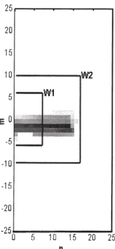
Although an infinite number of m and n indices are necessary for an exact result, a restricted number of Fou-rier modes provides an accurate solution. Thus, to ascer-tain whether there are enough modes, Gmn values are shown in the form of a map (the m and n are the coordi-nates of the map), which is useful for showing the impor-tance of each mode used for the numerical calculation of the UISNR. We call this map a “G-map” (see Fig. 4). Note that only positive n values are shown, because of the symmetry of the problem, i.e., Gmn ⫽ Gm(⫺n). One deter-mines the necessary number of modes by investigating the G-map with respect to the variable, n. The number of modes is decided according to the parameters of the body. For example, the number of modes increases as body length increases. We also observe that as the point of interest gets closer to the boundaries, a greater number of
FIG. 3. a: Sagittal H-map for the optimum coil. This map is produced on the plane, ⫽ 0, and the point of interest located at ( ⫽ 1 mm, ⫽ 0, z ⫽ 0) is indicated by a star. A logarithmic intensity scale is employed. b: Sensitivity magnitude profile for the opti-mum coil. H⫹ field sensitivity is plotted at
x ⫽ 1 mm in arbitrary units. Both figures
show that most of the field energy is con-centrated in a narrow region on the z-axis, and the greatest brightness indicates where the position of the internal coil should be.
modes in m and n indices are needed. Although this is the case for most points of interest, the values that determine body resistance, and eventually the UISNR values, are limited to a small range of m and n values; therefore, a finite sum of selected modes is acceptable. In Fig. 4, the total number of modes for both m and n is 1250, which is very high. Including all of these modes is time-consuming. If smaller m and n values are chosen, the window will get smaller, as shown in window 1 (W1) and W2. For W1, the numbers of m and n are insufficient, and the UISNR value obtained for this window (where m⫽ 6 and n ⫽ 7) is 33% less than the UISNR value of the largest window (m⫽ 50,
n⫽ 25). However, W2 (m ⫽ 10, n ⫽ 17) provides almost
the same UISNR value (a difference of 0.2%) as the largest window; thus, W2 includes the most effective modes and also requires much less time to plot the map. As a result, this mapping method is an efficient means of calculating the result.
Analysis of Loopless Antenna
The loopless antenna (10) is a very simple antenna design that has been investigated for use in MRI-guided vascular interventions (24). The design consists of a coaxial cable with an extended inner conductor. It is important to com-pare the UISNR values of the internal and external coils with the ISNR values of the loopless antenna in order to understand its performance. The UISNR value of the
in-ternal and exin-ternal coil combination was plotted for a 20-cm-radius body with a 0.375-mm-radius cavity as a function of the position of the point of interest in Fig. 5. The ISNR value of a loopless antenna (23), and the UISNR value that can be obtained from exclusively external coils were plotted on the same graph. By investigating this plot, one can see how much room for improvement there is in the SNR performance of the loopless antenna. In addition, we can determine which coil performs better in which region. For example, at a point of interest ( ⫽ 1 mm, ⫽ 0, z⫽ 0), the performance of the loopless antenna is only 4% of the UISNR of an internal and external coil combi-nation. This means that there may be an internal MRI coil design that fits in the same cavity and performs 25 times better than the loopless antenna for that point of interest. It is important to note that the coil design that can result in this significant improvement is not known at this time.
Deciding whether to use the loopless antenna for a spe-cific point of interest is crucial with regard to time-saving and therapeutic management. In Fig. 5, the SNR curve of the loopless antenna and the UISNR of the external coil intersect at one point. This point determines the radius of the “useful region” of an internal MRI coil, the loopless antenna. For points that are closer to the external surface of the body, some external coils, which perform better than the internal coil, may exist. The size of the useful region of an internal coil depends on the body radius. When the body size is large, the useful region of the internal coil increases, whereas when the body size is small, the inter-nal coil becomes useful for imaging a smaller region. Fig-ure 6 shows the radius of the useful area as a function of body size for the loopless antenna. To obtain this plot, we calculated the values of UISNR for external coils, and compared the SNR of the loopless antenna with the UISNR
FIG. 4. Relative importance of the modes (G-map). This is used for the numerical calculation of the UISNR. The weights of each mode were mapped on the horizontal and vertical axes, representing the
m and n modes, respectively. The restriction of the modes to those
encompassed by bound W2 speeds the calculation with a negligible loss of accuracy (⬍ 1%), whereas use of the overly-restrictive bound W1 results in a 33% error.
FIG. 5. A comparison of three ISNR values.0is the radial distance
of the point of interest from the center of the object. The internal coil is effective at points near the cavity, and then the external coil becomes effective as the point of interest approaches the outer boundary on the curve of the UISNR of an internal and external coil combination. In this figure, the external coil has a 20-cm body radius, and the internal and external coil combination has a 20-cm body radius and a 0.375-mm cavity radius. The radius of the loop-less antenna is 0.375 mm.
values as a function of body radius. For a fixed value of body radius, the SNR values were sampled at 5 mm, and the point where the loopless antenna SNR exceeded the UISNR for external coils was found by interpolation. The same procedure was repeated for different body radius values between 5 cm and 25 cm. Figure 6 shows that at any point of interest in the shaded area of the graph, the SNR of the loopless antenna dominates the UISNR of the exter-nal coil. This region is called the useful area of the loopless antenna. As a result, if the point of interest is in the shaded region, the loopless antenna should be used.
By comparing the loopless antenna with the UISNR of an internal and external coil combination, one can deter-mine how much improvement can be achieved over the loopless design, as well as determine the point of interest where the loopless antenna performs best. The ISNR val-ues for the loopless antenna were divided by the UISNR of an internal and external coil combination and plotted as a function of the point of interest in Fig. 7. Our sample design loopless antenna achieved maximum performance at the points of interest with a distance to the center of the body of⬃6.5 cm (0⫽ 6.5 cm). For those points, more than 20% of the maximum achievable SNR was obtained (see Fig. 7).
Analysis of Endourethral Coil Design
The endourethral coil design (12) is an elongated single loop that consists of a copper trace etched on a flexible circuit board. To calculate the ISNR values for the en-dourethral coil, we conducted a saline phantom experi-ment (FSE, ETL ⫽ 64, TR/TE ⫽ 10000/22 ms, matrix ⫽ 256⫻ 256, 1 NEX, slice thickness ⫽ 3 mm, FOV ⫽ 32 cm, BW ⫽ 62.5 kHz). Using the images of the phantom, we calculated the ISNR values as a function of radius for radial distances of 0.14 –15 cm. We measured the perfor-mance by dividing the experimental ISNR value of this coil by the UISNR value. UISNR values were computed for a 20-cm radius body with an internal cavity radius of 2.5 mm (the cavity size matched the endourethral coil diameter).
The experimental performance plots revealed that the performance of the single loop coil design reached 18% of its maximum, and that there is still significant room for improvement in this design (see Fig. 8). In addition, a comparison was made between the SNR of the single-loop endourethral coil and the UISNR value of the external
FIG. 6. The useful area for the loopless antenna. The SNR values of the loopless antenna and the UISNR of the internal and external coil combination were compared for different values of body radius,b.
For a given body radius, the loopless antenna outperforms the optimum external coil design for points of interest with0values that
fall in the shaded area. The region at the bottom left of the figure, shown by the dashed line, was found by interpolation.
FIG. 7. The performance of the loopless antenna as a function of distance of the point of interest from the center of the object. We obtained this figure by dividing the SNR of the loopless antenna by the UISNR of the internal and external coil combination. In this figure, a 20-cm body radius and a 0.375-mm cavity radius were assumed.
FIG. 8. The experimental performance of the endourethral coil de-sign as a function of distance of the point of interest from the center of the object. This figure shows the performance of a single-loop endourethral coil, which we determined by dividing the experimental SNR value of the coil by the UISNR of the internal coil. UISNR values were computed for a 20-cm radius body with an internal cavity radius of 2.5 mm (the cavity size matched the endourethral coil diameter).
coils (i.e., for the case of no cavity). This comparison revealed that at the position of ( ⫽ 1 cm, ⫽ 0, z ⫽ 0), the single-loop coil performs approximately 25 times bet-ter than any exbet-ternal coil.
Parameters for UISNR
Many parameters affect the UISNR of internal coils, such as the body radius b, cavity radius c, conductivity , relative electric permittivityεr, frequency , point of in-terest, and so forth. The point of interest was explored in detail in the previous section, and the frequency and cav-ity radius are examined in this section.
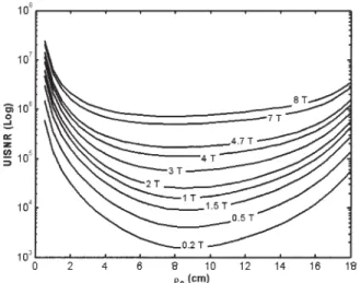
One of the main UISNR factors that affects the SNR is frequency, which is directly proportional to the field strength. Various magnetic field strengths between 0.2 and 8.0 tesla were used in the plot of Fig. 9. These values for magnetic field strengths (B) were chosen according to the values used for standard MRI systems. Quasi-static condi-tions are valid for regions near the boundaries where there is a linear relation between UISNR and the field strength. On the other hand, when the point of interest is away from the surface, UISNR increases faster with respect to fre-quency, as stated in Ref. 15. As frequency increases, the curvature of the curves becomes smaller. At 8 tesla, for the points of interest with radial distances from the center between 6 and 12 cm, the curve approaches a flat line. This behavior can be attributed to SNR gain due to focusing effects at high fields.
The cavity size is another important parameter for inter-nal coils. The UISNR values for an interinter-nal coil were plotted for various cavity values and a 20-cm body radius (see Fig. 10). The larger the cavity radius we used, the larger was the SNR at points close to the center.
While we were making the internal coil UISNR calcula-tions, we also made some other observations related to the use of internal coils. For example, we calculated the UISNR at a point of interest closer to the internal cavity for different body radius values, and found that the UISNR
value is weakly dependent on the body radius value. This shows that for a region of points inside the human body, a well-designed coil provide a similar performance, and is not strongly dependent on the size of the person being imaged. This can be explained by the fact that the effect of the external coil is negligible for points closer to the inter-nal cavity. Therefore, for this region, the position of the external coil (which depends on body size) does not really matter.
DISCUSSION
Different field distributions can be obtained for different points of interest. We observed that as the point of interest got closer to the outer boundary, the field distribution on the H-map became more effective (brighter) in the region close to the outer boundary. This can be explained by the fact that the internal coil loses its effect in that region. As a qualitative discussion, for the outer points, we can con-clude that external coils are more suitable for obtaining high SNR. Similarly, for the points of interest close to the internal cavity, the field was stronger at the inner regions. Therefore, for imaging inner points of the human body, internal coils are much more suitable. In addition, when a point of interest away from the origin is chosen, the H⫹ distribution of the field generated by the internal coil becomes uniform on the ⫽ 0 plane. This is because the effect of the internal coil is very weak, and the optimum field produced by the internal coil does not change the UISNR significantly. However, as the point of interest ap-proaches the inner region, the symmetry disappears and the internal coil field appears to be larger in magnitude.
Quasi-static conditions are effective when a point of interest is chosen at the region near the boundaries. In addition, as shown in Fig. 9, linearity can be observed when the point of interest is at a small cylindrical radius, i.e., at the region very close to the cavity.
FIG. 9. Frequency dependency of the UISNR at various magnetic field strengths. When the point of interest is at a small cylindrical radius, quasi-static conditions are valid, and there is then an ap-proximately linear relationship between the UISNR and field strength.
FIG. 10. The performance of coils with different cavity sizes. In this figure, different UISNR values for internal coils were compared for different cavity sizes. We made the comparison by dividing the UISNR values of various coils, which have different cavity radii, by the UISNR value of the reference coil, which has a cavity radius equal to 0.375 mm.
Mapping the field distribution can help guide the design of coils that have high SNR values close to the ultimate. In addition, the field distribution can roughly show the re-gions where the external and internal coils have negligible effects. For instance, for a point of interest where high-field magnitudes are obtained near the internal and exter-nal boundaries, both an interexter-nal and an exterexter-nal coil should be used to obtain an ultimate SNR value. For the maps, which show brightness only near the inner or outer boundaries, one type of coil would be enough.
The sagittal H-map (see Fig. 3) was produced on the ⫽ 0 plane with the point of interest ( ⫽ 1 mm, ⫽ 0, z ⫽ 0). In this figure, the highest brightness shows the position of the internal coil, located in the middle of the cylinder, in the z-direction. At 1 mm or more away from the origin in the z-direction, the field is very small with respect to the field at the center, if we ignore some fluctuations caused by truncation. The amplitude of these fluctuations gets even smaller when the truncation number is increased, suggest-ing that the optimum internal coil that might produce such magnetic field distribution is smaller in length.
Another important point to consider is the choice of a circular geometry. By employing a cylindrical geometry, we were able to use a cylindrical wave expansion. This simplified our computational analysis. We were also able to add to our model a cylindrical cavity for the UISNR computation of internal coils; however, in many medical applications for the internal coils, the body will not be circular and the cavity may not be centered.
Our sample designs (the loopless antenna and the en-dourethral coil) were found to be far from optimal. With another design, it should be possible to achieve at least a 10-fold SNR improvement. At this time, the geometry of the optimum coil design is unknown, but we believe that the results presented here will be useful for improving current coil designs and achieving the goal of determining the UISNR.
CONCLUSIONS
We have developed a method to calculate the ultimate value of the SNR that can be obtained with internal MRI coils. We propose to use this value as a reference to eval-uate the performance of internal MRI coils. As an example, we evaluated the performance of the endourethral coil and the loopless antenna, and assessed the extent of improve-ments required. In this work we employed cylindrical wave expansion, in which EM fields are represented by linear combinations of cylindrical waves. In addition, we compared our results with experimental results. Our work can be used as a reference for the performance of both internal and external coils.
ACKNOWLEDGMENT
We thank Ms. Mary McAllister for her valuable editorial support.
APPENDIX A
The longitudinal components of the electric and magnetic field are given in Eqs. [3] and [4]. By applying these
equa-tions to Eq. [6], the other components of the electric and magnetic fields can be calculated as follows:
Electric Fields Emn⫽
再
mzn n2 关AmnJm共n兲 ⫹ CmnYm共n兲兴 ⫹ n关BmnJ⬘m共n兲 ⫹ DmnY⬘m共n兲兴冎
e jme⫺jznz [24] Emn⫽再
m 2 ⬘n2 关BmnJm共n兲 ⫹ DmnYm共n兲兴 ⫺jzn n关AmnJ⬘m共n兲 ⫹ CmnY⬘m共n兲兴冎
e jmejznz [25] Magnetic Fields Hmn⫽再
⫺jmzn n2 关BmnJm共n兲 ⫹ DmnYm共n兲兴 ⫺⬘ n关AmnJ⬘m共n兲 ⫹ CmnY⬘m共n兲兴冎
e jme⫺jznz [26] Hmn⫽再
⫺ m2 n2 关AmnJm共n兲 ⫹ CmnYm共n兲兴 ⫺zn n关BmnJ⬘m共n兲 ⫹ DmnY⬘m共n兲兴冎
e jme⫺jznz [27] where⬘ ⫽ ( ⫹ jε) ⫽ j2/, and: J⬘m共n兲 ⫽ m Jm共n兲 ⫺ Jm⫹1共n兲 [28] Y⬘m共n兲 ⫽ m Ym共n兲 ⫺ Ym⫹1共n兲 [29] APPENDIX BThe components of H⫹ can be calculated by using the equation H⫹ ⫽ (H ⫺ jH )/公2, and Eqs. [26] and [27]. Using Eq. [9], the components of bᠬmn(rᠬ) ⫽ [bA , bB, bC,
bD]mn can be evaluated as:
bA共Jm, Jm⫹1兲 ⫽ 关⫺Jm共2/2兲共
冑
2m/兲 ⫹ Jm⫹1共2/兲共1/共冑
2兲兲兴ejme⫺jznz bB共Jm, Jm⫹1兲 ⫽ 关⫺Jm共z/2兲共冑
2m/兲 ⫹ Jm⫹1共z/兲共1/冑
2兲兴ejme⫺jznz bC共Ym, Ym⫹1兲 ⫽ 关⫺Ym共2/2兲共冑
2m/兲 ⫹ Ym⫹1共2/兲共1/共冑
2兲兲兴ejme⫺jznz bD共Ym, Ym⫹1兲 ⫽ 关⫺Ym共z/2兲共冑
2m/兲 ⫹ Ym⫹1共z/兲共1/冑
2兲兴ejme⫺jznz [30]REFERENCES
1. Schnell W, Renz W, Vester M, Ermert H. Ultimate signal-to-noise ratio of surface and body antennas for magnetic resonance imaging. IEEE Trans Ant Prop 2000;48:418 – 428.
2. Kowalski ME, Jin JM, Chen J. Computation of the signal-to-noise ratio of high-frequency magnetic resonance imagers. IEEE Trans Biomed Eng 2000;47:1525–1533.
3. Martin A, Plewes D, Henkelman R. MR imaging of blood vessels with an intravascular coil. J Magn Reson Imaging 1992;2:421– 429. 4. Hurst GC, Hua J, Duerk JL, Cohen AM. Intravascular (catheter) NMR
receiver probe: preliminary design analysis and application to canine iliofemoral imaging. Magn Reson Med 1992;24:343–357.
5. Kantor H, Briggs R, Balaban R. In vivo 31P nuclear magnetic resonance measurements in canine heart using a catheter-coil. Circ Res 1984;55: 261–266.
6. Quick HH, Ladd ME, Hilfiker PR, Paul GG, Ha SW, Debatin JF. Au-toperfused balloon catheter for intravascular MR imaging. J Magn Re-son Imaging 1999;9:428 – 434.
7. Martin AJ, McLoughlin RF, Chu KC, Barberi EA, Rutt BK. An expand-able intravenous RF coil for arterial wall imaging. J Magn Reson Imag-ing 1998;8:226 –234.
8. Schnall MD, Lenkinski RE, Pollack HM, Imai Y, Kressel HY. Prostate: MR imaging with an endorectal surface coil. Radiology 1989;172:570 – 574.
9. Atalar E, Bottomley PA, Ocali O, Correia LCL, Kelemen MD, Lima JAC, Zerhouni EA. High resolution intravascular MRI and MRS by using a catheter receiver coil. Magn Reson Med 1996;36:596 – 605.
10. Ocali O, Atalar E. Intravascular magnetic resonance imaging using a loopless catheter antenna. Magn Reson Med 1997;37:112–118. 11. Shunk KA, Lima JAC, Heldman AW, Atalar E. Transesophageal
mag-netic resonance imaging. Magn Reson Med 1999;41:722–726.
12. Quick HH, Serfaty JM, Pannu HK, Genadry R, Yeung CJ, Atalar E. Endourethral MRI. Magn Reson Med 2001;45:138 –146.
13. Kandarpa K, Jakab P, Patz S, Schoen FJ, Jolesz FA. Prototype miniature endoluminal MR imaging catheter. J Vasc Intervent Radiol 1993;4:419 – 427.
14. Schnall MD, Imai Y, Tomaszewski J, Pollack HM, Lenkinski RE, Kressel HY. Prostate cancer: local staging with endorectal surface coil MR imaging. Radiology 1991;178:797– 802.
15. Ocali O, Atalar E. Ultimate intrinsic signal-to-noise ratio in MRI. Magn Reson Med 1998;39:462– 473.
16. Edelstein WA, Glover GH, Hardy CJ, Redington RW. The intrinsic signal-to-noise ratio in NMR imaging. Magn Reson Med 1986;3:604 – 618.
17. Abdel-Hafez IA. UISNR in MRI by optimizing EM field generated by internal coils M.S. thesis, Bilkent University, Ankara, Turkey, 2000. 18. Veselle H, Collin RE. The signal-to-noise ratio of nuclear
magnetic-resonance surface coils and application to a lossy dielectric cylinder model 1. Theory. IEEE Trans Biomed Eng 1995;42:497–506. 19. Vesselle H, Collin RE. The signal-to-noise ratio of nuclear
magnetic-resonance surface coils and application to a lossy dielectric cylinder model 2. The case of cylindrical window coils. IEEE Trans Biomed Eng 1995;42:507–520.
20. Hoult DI, Richards RE. The signal-to-noise ratio of the nuclear magnetic resonance experiment. J Magn Reson 1976;24:71– 85.
21. Morse PM, Feshbach H. Green’s functions. Methods of theoretical physics. Vol. I. New York: McGraw Hill; 1953. p 832.
22. Balanis CA. Advanced engineering electromagnetics. New York: Wiley; 1989.
23. Susil RC, Yeung CJ, Atalar E. Intravascular extended sensitivity (IVES) MRI antennas. Magn Reson Med 2003;50:383–390.
24. Serfaty JM, Yang XM, Foo TK, Kumar A, Derbyshire A, Atalar E. MRI-guided coronary catheterization and PTCA: a feasibility study on a dog model. Magn Reson Med 2003;49:258 –263.