CACHE LOCALITY EXPLOITING METHODS AND
MODELS FOR SPARSE MATRIX-VECTOR
MULTIPLICATION
A THESIS SUBMITTED TO
THE DEPARTMENT OF COMPUTER ENGINEERING AND INFORMATION SCIENCE
AND THE INSTITUTE OF ENGINEERING AND SCIENCE OF BILKENT UNIVERSITY
IN PARTIAL FULFILLMENT OF THE REQUIREMENTS FOR THE DEGREE OF
MASTER OF SCIENCE
By
Kadir Akbudak
September, 2009
I certify that I have read this thesis and that in my opinion it is fully adequate, in scope and in quality, as a thesis for the degree of Master of Science.
Prof. Cevdet Aykanat (Advisor)
I certify that I have read this thesis and that in my opinion it is fully adequate, in scope and in quality, as a thesis for the degree of Master of Science.
Prof. Ayhan Altıntas¸
I certify that I have read this thesis and that in my opinion it is fully adequate, in scope and in quality, as a thesis for the degree of Master of Science.
Asst. Prof. ¨Ozcan ¨Ozt¨urk
Approved for the Institute of Engineering and Science:
Prof. Mehmet Baray Director of the Institute
ABSTRACT
CACHE LOCALITY EXPLOITING METHODS AND
MODELS FOR SPARSE MATRIX-VECTOR
MULTIPLICATION
Kadir AkbudakMaster in Computer Engineering and Information Science Supervisor: Prof. Cevdet Aykanat
September, 2009
The sparse matrix-vector multiplication (SpMxV) is an important kernel operation widely used in linear solvers. The same sparse matrix is multiplied by a dense vec-tor repeatedly in these solvers to solve a system of linear equations. High performance gains can be obtained if we can take the advantage of today’s deep cache hierarchy in SpMxV operations. Matrices with irregular sparsity patterns make it difficult to utilize data locality effectively in SpMxV computations. Different techniques are pro-posed in the literature to utilize cache hierarchy effectively via exploiting data local-ity during SpMxV. In this work, we investigate two distinct frameworks for cache-aware/oblivious SpMxV: single matrix-vector multiply and multiple submatrix-vector multiplies. For the single matrix-vector multiply framework, we propose a cache-size aware top-down row/column-reordering approach based on 1D sparse matrix parti-tioning by utilizing the recently proposed appropriate hypergraph models of sparse matrices, and a cache oblivious bottom-up approach based on hierarchical clustering of rows/columns with similar sparsity patterns. We also propose a column compres-sion scheme as a preprocessing step which makes these two approaches cache-line-size aware. The multiple submatrix-vector multiplies framework depends on the partition-ing the matrix into multiple nonzero-disjoint submatrices. For an effective matrix-to-submatrix partitioning required in this framework, we propose a cache-size aware top-down approach based on 2D sparse matrix partitioning by utilizing the recently proposed fine-grain hypergraph model. For this framework, we also propose a trav-eling salesman formulation for an effective ordering of individual submatrix-vector multiply operations. We evaluate the validity of our models and methods on a wide range of sparse matrices. Experimental results show that proposed methods and mod-els outperforms state-of-the-art schemes.
iv
Keywords: Cache locality, sparse matrices, matrix-vector multiplication, matrix re-ordering, computational hypergraph model, hypergraph partitioning, traveling sales-man problem.
¨
OZET
SEYREK MATR˙IS-VEKT ¨
OR C
¸ ARPIMINDA
¨
ONBELLEK YERELL˙I ˘
G˙I SA ˘
GLAYAN Y ¨
ONTEM VE
MODELLER
Kadir AkbudakBilgisayar ve Enformatik M¨uhendisli˘gi, Master Tez Y¨oneticisi: Prof. Dr. Cevdet Aykanat
Eyl¨ul, 2009
Seyrek matris-vekt¨or c¸arpımı do˘grusal denklem sistemi c¸¨ozen yazılımlarda c¸ok ¨onemli bir c¸ekirdek is¸lemdir. Aynı seyrek matris, seyrek olmayan bir vekt¨orle c¸ok defa c¸arpılır. S¸u anki teknolojinin sundu˘gu c¸ok seviyeli ¨onbellekler etkin kullanılırsa, bu c¸arpma is¸lemi sırasında ¨onemli performans kazanc¸ları olabilmektedir. Lakin d¨uzensiz veri eris¸imine neden olan matrisler ¨onbellekteki veri yerelli˘ginin kullanımını olum-suz etkilemektedir. Bu problemi c¸¨ozmek ic¸in ¨onbellek yerelli˘gini kullanan pek c¸ok y¨ontem s¸u zamana kadar sunulmus¸tur. Bu c¸alıs¸mada, biz de iki farklı c¸erc¸eve sunuy-oruz: tek matris-vektor c¸arpımı ve c¸oklu matris-vektor c¸arpımı. Tek matris-vekt¨or c¸arpımı c¸erc¸evesinde, ¨onbelle˘gin boyutunu dikkate alarak matrisin satır ve s¨utunlarını yeniden sıralayan ve bu sıralama is¸lemini hiperc¸izge b¨ol¨umleme ile yapan bir y¨ontem sunuyoruz. Bir de ¨onbelle˘gin boyutunu dikkate almadan yerelli˘gi sa˘glayacak bir y¨ontem ¨oneriyoruz. Ve bu y¨ontemlere ek olarak s¨utunları sıkıs¸tırıp alansal yerelli˘gi sa˘glayan ¨onis¸leme y¨ontemi sunuyoruz. C¸ oklu matris-vekt¨or c¸arpımı c¸erc¸evesinde, ma-trisi alt matrislere ayırarak veri yerelli˘gini sa˘glamaya c¸alıs¸mayı hedefliyoruz. Yine bu ayırma is¸leminde de hiperc¸izge kullanılıyor. Alt matrislerin c¸arpma sırası da ¨onem tas¸ıdı˘gından veri yerelli˘gini arttıran bir sıralamayı bulma problemini de seyyar satıcı problemi olarak c¸¨oz¨ulebilece˘gini ac¸ıklıyoruz. Deneysel sonuc¸lar bu ¨onerilen c¸erc¸eve ve y¨ontemlerin s¸u anda kullanılan y¨ontemlerden daha hızlı c¸alıs¸tı˘gını g¨ostermektedir.
Anahtar s¨ozc¨ukler: ¨Onbellek yerelli˘gi, seyrek matrisler, matris-vekt¨or c¸arpımı, matrisi yeniden sıralama, bilis¸imsel hiperc¸izge modeli, hiperc¸izge b¨ol¨umleme, seyyar satıcı problemi .
Acknowledgement
I would like to express my deepest gratitude to my supervisor Prof. Cevdet Aykanat for his guidance, suggestions, and invaluable encouragement throughout the develop-ment of this thesis. His patience, motivation, lively discussions and cheerful laughter provided an invaluable and comfortable atmosphere for our work.
I am grateful to my family and my friends for their infinite moral support and help. I owe special thanks to my friend Enver Kayaaslan.
Finally, I thank T ¨UB˙ITAK for supporting grant throughout my master program.
To my family
Contents
1 Introduction 1
2 Background 4
2.1 Data Storage Schemes used in Sparse Matrix-Vector Multiplication . . 4
2.1.1 Compressed Storage by Rows . . . 5
2.1.2 Zig-Zag Compressed Storage by Rows . . . 6
2.1.3 Incremental Compressed Storage by Rows . . . 7
2.1.4 Zig-Zag Incremental Compressed Storage by Rows . . . 8
2.2 Data Locality in Sparse Matrix-Vector Multiply . . . 8
2.3 Hypergraph Partitioning . . . 9
2.4 Hypergraph Models for Sparse Matrix Partitioning . . . 11
2.5 Breadth-First-Search-Based Algorithm for Row/Column Reordering . 13 2.6 Travelling Salesman Problem . . . 14
3 Related Work 16
4 Single Matrix-Vector Multiply Framework 19
CONTENTS ix
4.1 1D Decomposition of Sparse Matrices . . . 20
4.2 Hierarchical Clustering . . . 21
4.3 Compression Preprocessing for Spatial Locality . . . 23
5 Multiple Submatrix-Vector Multiplies Framework 25 5.1 Pros and Cons compared to Conventional Framework . . . 26
5.2 2D Decomposition of Sparse Matrices . . . 29
5.3 Ordering Submatrix-Vector Multiplies . . . 29
6 Experimental Results 32 6.1 Experimental Setup . . . 32
6.1.1 Platform . . . 33
6.1.2 Data Sets . . . 33
6.2 Experiments with Single Matrix-Vector Multiply Framework . . . 35
6.3 Experiments with Multiple Submatrix-Vector Multiplies Framework . 39 6.4 Comparison of Frameworks . . . 39
7 Conclusion 41 7.1 Conclusions . . . 41
7.2 Future Work . . . 42
Appendices 44
CONTENTS x
List of Figures
2.1 Processing order of nonzeros stored using the CSR (on the left) and ZZCSR (on the right) schemes. Arrows denote the storage order of
nonzeros of a row. . . 6
3.1 Example for irregular code that are the focus in computation and data ordering problem. C array is accessed through two index arrays a andb. These two arrays cause indirection so the code shows irregular access patter. . . 17
3.2 Sparse matrix-vecto multiply algorithm based on using the CSR scheme. x array is the x-vector in the sparse matrix-vector multiplica-tiony ← Ax . . . 18
B.1 Original Matrix psse1 . . . 47
B.2 Partitioned Matrix psse1 whenB = 1 and K = 2 . . . 48
B.3 Partitioned Matrix psse1 whenB = 2 and K = 4 . . . 49
B.4 Partitioned Matrix psse1 whenB = 3 and K = 8 . . . 50
B.5 Partitioned Matrix psse1 whenB = 4 and K = 16 . . . 51
List of Tables
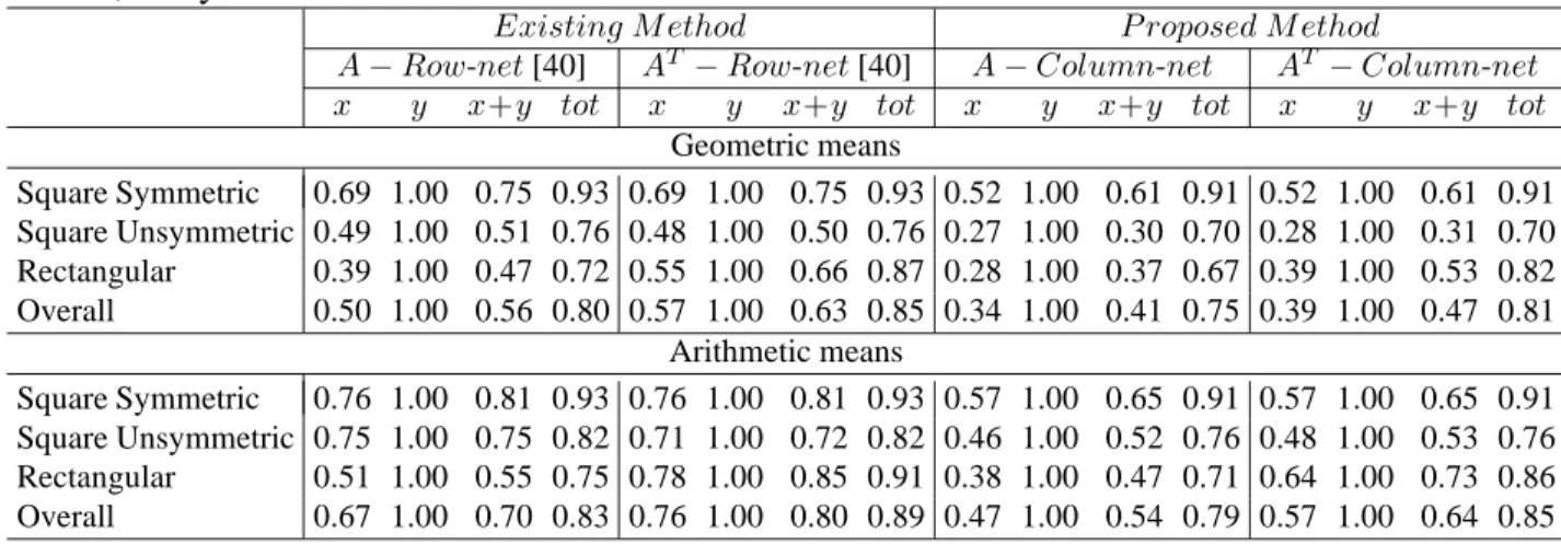
6.1 Properties of test matrices. . . 34 6.2 Normalized geometric and arithmetic means of simulation results for
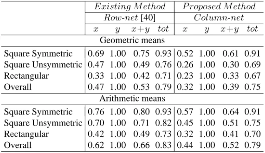
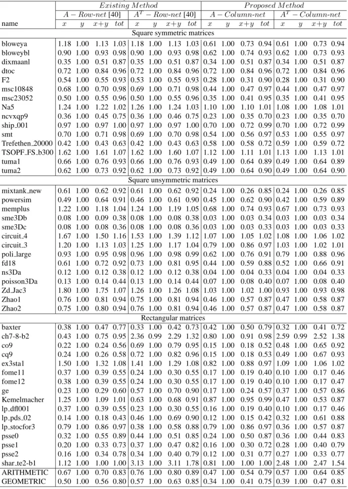
matrices partitioned into 32K-sized parts using row-net and column-net models. Original matrices are partitioned and their transposes, too. Cache line size is 8 times size of double, 64Bytes. . . 36 6.3 Normalized geometric and arithmetic means of simulation results for
matrices partitioned into 32K-sized parts using row-net and column-net models. Best result of either original matrix or its transpose is selected. Cache line size is 8 times size of double, 64Bytes. . . 37 6.4 Normalized geometric and arithmetic means of simulation results for
matrices partitioned into 32K-sized parts using row-net and column-net models; and matrices reordered using BFS and Hierarchical algo-rithms . . . 37
LIST OF TABLES xiii
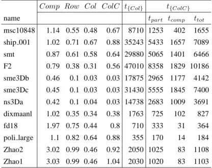
6.5 Normalized simulation results for some matrices. Results for only compression method applied are inComp column. Results for
matri-ces are partitioned into 32K-sized parts using column-net model with-out column reordering are in Row column; with column ordering in Col. Results for column-net model without column reordering but
with compression are in ColC column. Time elapsed for reordering
and compression are measured in milliseconds. Timing results for re-ordering using column-net model int{Col}column. Compression, par-titioning and total times for reordering using column-net model with-out column reordering but with compression are given separately in
t{ColC}column. . . 38 6.6 Normalized geometric and arithmetic means of simulation results
for matrices partitioned into 32K-sized parts using fine-grain model.
NOT SP column contains results when TSP ordering not used.Cache
line size is 8 times size of double, 64Bytes. . . 39 6.7 Normalized geometric and arithmetic means of simulation results for
matrices partitioned into 32K-sized parts using column-net model and fine-grain model with TSP ordering. . . 40
A.1 Simulation results for matrices partitioned into 32K-sized parts. Cache line size is 8 times size of double, 64Bytes. . . 45
List of Algorithms
1 Sparse Matrix-Vector Multiplication using CSR scheme . . . 6
2 Sparse Matrix-Vector Multiplication using ICSR scheme . . . 7
3 Modified BFS Algorithm for Row/Column Ordering . . . 14
4 Hypergraph Based Bottom-up Reordering HPART . . . 24
5 Hypergraph Based Clustering HCLUSTER . . . 24 6 Multiple Sparse Submatrix-Vector Multiplications using ICSR scheme 26
Chapter 1
Introduction
Many applications became available in numerical computation on behalf of the devel-opments in computer architecture. Nevertheless, these develdevel-opments introduced some problems such as performance gap between processor and memory speeds. Also there still exits a trade-off between faster but small memories like cpu caches and slower but larger memories like RAM. As a result, the need of new methods and algorithms for efficient usage of higher levels of memory increased in every area of computational problems.
Efficiency in using higher level memories mainly depend on temporal and spatial localities. According to literature, these localities are provided throughout these two ways: data ordering and iteration ordering.
Here data ordering means in what order the elements are stored; and in the same way, iteration ordering means in which order the stored elements are processed. When the data in consecutive memory locations is accessed with stride one, both spatial and temporal localities can be exploited even in compilers. Such kind of applications are said to be regular. On the contrary, it is considerable difficult to utilize the data locality effectively in irregular computations which induce irregular memory access patterns.
The sparse matrix-vector multiplication is one of them and the most important kernel operation in linear solvers for the solution of large, sparse, linear systems of equations. These solvers repeat the matrix-vector multiplication y ← Ax many times
with the same sparse matrix to solve a system of equations. Irregular access pattern 1
CHAPTER 1. INTRODUCTION 2
during this multiply operation, causes poor usage of cpu caches in today’s memory hi-erarchy technology. However, sparse matrix-vector multiply operation has a potential to exhibit very high performance gains when temporal and spatial localities discussed in Section 2.2 are respected and exploited.
In this work, we investigate two distinct frameworks for cache-aware/oblivious Sp-MxV: single matrix-vector multiply and multiple submatrix-vector multiplies. For the single matrix-vector multiply framework, we propose a cache-size aware top-down row/column-reordering approach based on transformation a sparse matrix to a singly-bordered block-diagonal form by utilizing the recently proposed appropriate hyper-graph models. We provide an upper bound on the total number of cache misses based on this transformation, and show that the objective in the hypergraph-partitioning-based transformation model exactly corresponds to minimizing this upper bound. We also propose a cache oblivious bottom-up approach based on hierarchical clustering of rows/columns with similar sparsity patterns. Furthermore, a column compression scheme as a preprocessing step which makes these two approaches cache-line-size aware is presented.
The multiple submatrix-vector multiplies framework depends on the partitioning the matrix into multiple nonzero-disjoint submatrices and the ordering of submatrix-vector multiplies. For an effective matrix-to-submatrix partitioning required in this framework, we propose a cache-size aware top-down approach based on 2D sparse matrix partitioning by utilizing the recently proposed fine-grain hypergraph model. We provide an upper bound on the total number of cache misses based on this matrix-to-submatrix partitioning, and show that the objective in the hypergraph-partitioning-based matrix-to-submatrix partitioning exactly corresponds to minimizing this upper bound.
For this framework, we also propose a traveling salesman formulation for an effec-tive ordering of individual submatrix-vector multiply operations. We provide a lower bound on the total number of cache misses based on the ordering of submatrix-vector multiplies, and show that the objective in TSP formulation exactly corresponds to min-imizing this lower bound.
We evaluate the validity of our models and methods on a wide range of sparse matrices. Experimental results show that proposed methods and models outperforms
CHAPTER 1. INTRODUCTION 3
state-of-the-art schemes.
The rest of this thesis is organized as follows: Background material is introduced in Chapter 2. In Chapter 3, we review some of the previous works about iteration/data reordering and matrix transformations for exploting locality. Two frameworks as our contributions in sparse matrix-vector multiplication are described in Chapters 4 and 5. We present the experimental results of these two frameworks and comparisons with some of the previous works in Chapter 6. Finally, the thesis is concluded in Chapter 7.
Chapter 2
Background
In this chapter, we will review several schemes for storing sparse matrices in Sec-tion 2.1. Data locality issues during matrix-vector multiplicaSec-tion will be considered in Section 2.2. Then we will review definition of hypergraph and partitioning prob-lems in Section 2.3. We will mention about two hypergraph models for 1D and 2D decomposition of sparse matrices in Section 2.4. Finally, definition of the well known Travelling Salesman Problem (TSP) will be told in Section 2.6.
2.1
Data Storage Schemes used in Sparse
Matrix-Vector Multiplication
In this chapter we will review an important storage scheme Compressed Storage by Rows (CSR) and its variances, Zig-Zag Compressed Storage by Rows (ZZCSR), In-cremental Compressed Storage by Rows (ICSR) and Zig-Zag InIn-cremental Compressed Storage by Rows (ZZICSR) for sparse matrix-vector multiplication in Sections 2.1.1, 2.1.2,2.1.3 and 2.1.4, respectively.
There are two main storage schemes for sparse matrix-vector multiply opera-tion. They are Compressed Storage by Rows (CSR) and Compressed Storage by Columns (CSC) [12, 34]. Each sparse-matrix storage scheme determines a distinct computation scheme for the matrix-vector multiplication. In this thesis, we restrict our
CHAPTER 2. BACKGROUND 5
focus on cache-aware/oblivious computation of sparse matrix-vector multiply opera-tion using the CSR storage scheme without loss of generality.
In the following subsections we review four CSR-based sparse-matrix storage schemes.
1. CSR
2. Zig-zag CSR 3. ICSR
4. Zig-zag ICSR
For other types of schemes, books such as Duff, Erisman, and Reid [14] can be inves-tigated.
2.1.1
Compressed Storage by Rows
CSR scheme is widely used in sparse matrix operations. In this scheme and in all the remaining schemes mentioned in this section, only the nonzeros are naively stored without using any structural information. Nonzeros are stored in a row-major format, meanly nonzeros of a row are stored consecutively. This scheme contains three ar-rays: nonzero, column-index and row-start. The values and the column indices of the nonzeros are stored in row-major order in the nonzero and column-index arrays in
one-to-one manner, respectively. That is, column-index[i] stores the column-index
of the nonzero and the value of this nonzero is stored in nonzero[i]. The row-start
array stores the index of the first nonzero element of each row. This index is used to access both of nonzero and column-index arrays. Also the original row order of the sparse matrix A is preserved while constructing row-start array and similarly the
original column order is preserved while constructing nonzero and column-index ar-rays; but these preservations of the original orders are not obligatory, we will assume these original orderings in this work. Algorithm 1 shows how the sparse matrix-vector multiplication can be performed using CSR storage scheme.
CHAPTER 2. BACKGROUND 6
Algorithm 1 Sparse Matrix-Vector Multiplication using CSR scheme
Require: nonzero , column -index and row -start arrays of a m by n sparse matrix A
a dense input vector x
1: for i← 1 to m do
2: tmp← 0
3: for j ← row -start[i] to row -start[i + 1] − 1 do
4: tmp← tmp + nonzero[i] ∗ x[column-index[j]]
5: end for
6: y[i] ← tmp
7: end for
8: return y
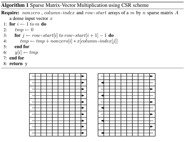
Figure 2.1: Processing order of nonzeros stored using the CSR (on the left) and ZZCSR (on the right) schemes. Arrows denote the storage order of nonzeros of a row.
2.1.2
Zig-Zag Compressed Storage by Rows
Zig-zag CSR (ZZCSR) scheme [40] is similar to CSR. In CSR scheme, multiplication is being performed through increasing index on each row. In ZZCSR, multiplication is being performed through increasing index on even-numbered rows and through de-creasing index on odd-numbered rows. In this way, possibility of reuse of recently retrieved x-vector entries in cache is increased. Figure 2.1 illustrates comparison of
these two schemes. This ZZCSR scheme can be simply implemented by reversing the order of elements in nonzero and column-index arrays of odd-numbered rows in the CSR scheme.
CHAPTER 2. BACKGROUND 7
2.1.3
Incremental Compressed Storage by Rows
Incremental Compressed Storage by Rows (ICSR) proposed in [25] and it is reported to decrease instruction overhead by using pointer arithmetic. In addition, the idea behind this storage scheme perfectly fits for matrices having empty rows. In the CSR scheme, all rows, whether they are empty or not, must be present in the row-start array. But in ICSR, row indices of the empty rows are not stored at all, because row indices and column indices are calculated by accumulating elements of row-jump and column-diff arrays on current values. In contrast, these indices are retrieved from row-start and column-index arrays in CSR scheme. In other words, index of the next row ri to be processed is calculated by adding row-jump[i] to the current row index value. In the same way, the index of the next column cj to be processed is calculated by adding column-diff[j] to the current column index value. Then, row increments are triggered just after column index value becomes greater than number of columns. The number of columns is subtracted from overflowed column index value and used as new column index. New row index is calculated using related element of row-jump array and current row index value. These steps can be easily understood from Algorithm 2. Algorithm 2 Sparse Matrix-Vector Multiplication using ICSR scheme
Require: nonzero , column -diff and row -jump arrays of a m by n sparse matrix A
a dense input vector x
number of nonzeros nnz in matrix A
1: i← row -jump[0] 2: j← column-diff [0] 3: k← 0 4: r ← 1 5: tmp← 0 6: while k < nnz do 7: tmp← tmp + nonzero[k] ∗ x[j] 8: k← k + 1 9: j← j + column-diff [k] 10: if j ≥ n then 11: y[i] ← tmp 12: tmp← 0 13: j← j − n 14: i← i + row -jump[r] 15: r ← r + 1 16: end if 17: end while 18: return y
CHAPTER 2. BACKGROUND 8
2.1.4
Zig-Zag Incremental Compressed Storage by Rows
Zig-Zag Incremental Compressed Storage by Rows (ZZICSR) [40] combines CSR and zig-zag property. Temporal locality in x-vector is exploited using the zig-zag
prop-erty. In addition to this, empty rows are not stored. As a result, this scheme becomes convenient for sparse matrices having a considerable amount of empty rows as well as the temporal locality is achieved for x-vector . Like ZZCSR scheme, this scheme
can be implemented by putting negative values in row-jump and column-index arrays of odd-numbered rows in the ICSR scheme. So that flow of process is reversed in odd-numbered rows.
2.2
Data Locality in Sparse Matrix-Vector Multiply
Here, we will briefly mention about the data locality characteristics of matrix-vector multiply operation y ← Ax using the CSR scheme as also discussed in [39]. In terms
of the A-matrix stored in CSR format, temporal locality is not feasible since the
ele-ments of each of thenonzero, column-index (column-diff in ICSR) and row -start
(row -jump in ICSR) arrays are accessed only once. Spatial locality is feasible and it
is achieved automatically by nature of the CSR scheme since the elements of each of the three arrays are stored and accessed consecutively.
In terms of output vector y , temporal locality is not feasible since each y -vector
result is written only once to the memory. As a different view [39], temporal locality can be considered as feasible but automatically achieved at the register level. Spatial locality is feasible and it is achieved automatically since they -vector entry results are
stored consecutively.
In terms of input vector x, both temporal and spatial locality are feasible.
Tem-poral locality is feasible since each x-vector entry may be accessed multiple times.
However, exploiting the temporal and spatial locality for the x-vector is the major
concern in the CSR scheme since x-vector entries are accessed through a column-index array (column-diff in ICSR) in a non-contiguous manner.
CHAPTER 2. BACKGROUND 9
the exploitation level of these data localities depends both on the existing sparsity pattern of matrixA and the effectiveness of reordering heuristics.
2.3
Hypergraph Partitioning
A hypergraph H = (V, N ) is defined as a set of vertices V and a set of nets
(hyper-edges) N . Every net nj ∈ N connects a subset of vertices, i.e., nj⊆ V . The vertices connected by a net nj are called its pins (i.e., P ins(nj)). Weights can be associated with the vertices. We use w(vi) to denote the weight of the vertex vi.
Given a hypergraph H = (V, N ), Π = {V1, . . . , VK} is called a K -way partition of the vertex set V if each part is nonempty, i.e., Vk 6= ∅ for 1 ≤ k ≤ K ; parts are pairwise disjoint, i.e., Vk∩ Vℓ = ∅ for 1 ≤ k < ℓ ≤ K ; and the union of parts gives
V , i.e., S
kVk = V . A K -way vertex partition of H is said to satisfy the partitioning constraint if
Wk ≤ Wavg(1 + ε), for k = 1, 2, . . . , K (2.1)
In here, the weight Wk of a part Vk is defined as the sum of the weights of the ver-tices in that part (i.e., Wk =
P
vi∈Vkw(vi)), Wavg is the average part weight (i.e.,
Wavg= (Pvi∈Vw(vi))/K ), and ε represents the predetermined, maximum allowable
imbalance ratio.
In a partition Π of H, a net that connects at least one pin (vertex) in a part is said
to connect that part. Connectivity set Λj of a net nj is defined as the set of parts connected by nj. Connectivity λj = |Λj| of a net nj denotes the number of parts connected bynj. A net nj is said to be cut (external) if it connects more than one part (i.e., λj > 1), and uncut (internal) otherwise (i.e., λj = 1). The set of external nets of a partition Π is denoted as NE. The partitioning objective is to minimize the cutsize defined over the cut nets. There are various cutsize definitions. The relevant definition is:
CHAPTER 2. BACKGROUND 10
cutsize(Π) = X
nj∈NE
(λj − 1) (2.2)
In here, each cut net nj contributesλj− 1 to the cutsize. The hypergraph partitioning problem is known to be NP-hard [27].
Recently, multilevel HP approaches [4, 19, 21] have been proposed, leading to suc-cessful HP tools hMetis [23] and Patoh [7]. These multilevel heuristics consist of 3 phases: coarsening, initial partitioning, and uncoarsening. In the first phase, a mul-tilevel clustering is applied starting from the original hypergraph by adopting various matching heuristics until the number of vertices in the coarsened hypergraph decreases below a predetermined threshold value. Clustering corresponds to coalescing highly interacting vertices to supernodes. In the second phase, a partition is obtained on the coarsest hypergraph using various heuristcs including FM, which is an iterative refine-ment heuristic proposed for graph/hypergraph partitioning by Fiduccia and Matthey-ses [15] as a faster implementation of the KL algorithm proposed by Kernighan and Lin [24]. In the third phase, the partition found in the second phase is successively projected back towards the original hypergraph by refining the projected partitions on the intermediate level uncoarser hypergraphs using various heuristics including FM.
The recursive bisection (RB) paradigm is widely used in K -way hypergraph
par-titioning and known to be amenable to produce good solution qualities. In the RB paradigm, first, a two-way partition of the hypergraph is obtained. Then, each part of the bipartition is further bipartitioned in a recursive manner until the desired num-ber K of parts is obtained or part weights drop below a given maximum allowed part
weightWmax. In RB-based hypergraph partitioning, the cut-net splitting scheme [6] is adopted to capture theλ − 1 cutsize metric given in Equation 2.2. In hypergraph
par-titioning, balancing the part weights of the bipartition is enforced as the bipartitioning constraint.
The RB paradigm is inherently suitable for partitioning hypergraphs when K is not known in advance. Hence, the RB paradigm can be successfully utilized in clustering rows/columns for cache-size aware row/column reordering.
CHAPTER 2. BACKGROUND 11
2.4
Hypergraph Models for Sparse Matrix
Partition-ing
Recently, several successful hypergraph models and methods are proposed for efficient parallelization of sparse matrix-vector multiplication [5, 6, 9]. The relevant ones are row-net, column-net, and row-column-net models. The row-net and column-net mod-els are proposed and used for 1D rowwise and 1D columnwise partitioning of sparse matrices, respectively, whereas row-column-net model is used for 2D fine-grain parti-tioning of sparse matrices.
In the row-net hypergraph model [5, 6, 9] HRN(A) = (VC, NR) of matrix A, there exist one vertex vj ∈ VC and one net ni ∈ NR for each column cj and row ri, respectively. The vertex vj represents the DAXPY-like operation which multiplies xj with columncj and adds the result of this scalar-vector product to the output vector y . The weight w(vj) of a vertex vj∈ VR is set to the number of nonzeros in column cj. The net ni connects the vertices corresponding to the columns that have a nonzero entry in row ri. That is, vj∈ P ins(ni) if and only if aij6= 0. Here, ni represents the
y -vector entry yi andP ins(ni) represents the set of scalar multiply results needed to be accumulated in yi during matrix-vector multiply.
In the column-net hypergraph model [5, 6, 9] HCN(A) = (VR, NC) of matrix A, there exist one vertex vi ∈ VR and one net nj ∈ NC for each row ri and column cj, respectively. The vertexvi represents the inner product of row ri with the input vector
x. The weight w(vi) of a vertex vi∈ VR is set to the number of nonzeros in row ri. Net nj connects the vertices corresponding to the rows that have a nonzero entry in column cj. That is, vi ∈ P ins(nj) if and only if aij 6= 0. Here, nj represents the
x-vector entry xj and P ins(nj) represents the set of inner product operations that need xj during matrix-vector multiply.
In the row-column-net model [8] (also called as fine-grain model) HRCN(A) =
(VZ, NRC) of matrix A, there exists one vertex vij ∈ VZ corresponding to each nonzero aij in matrix A. In net set NRC, there exists a row-net nri for each row
ri, and there exists a column-netnci and for each columncj. The vertex vij represents the scalar multiply-and-add operation yij ← aijxj. Therefore each vertex is assigned unit weight. The row-netnr
CHAPTER 2. BACKGROUND 12
rowri, and the column-net ncj connects the vertices corresponding to the nonzeros in the column cj. That is, vij∈ P ins(nir) and vij∈ P ins(nrj) if and only if aij6= 0. Note that each vertex vij is a pin of exactly two nets. Here, ncj represents xj and P ins(ncj) represents the set of scalar multiply-and-add operations that needxj, whereas nri rep-resents yi and P ins(nri) represents the set of scalar multiply-and-add results needed to accumulate yi.
The use of the hypergraphs HRN(A), HCN(A) and HRCN(A) in sparse matrix partitioning for parallelization of matrix-vector multiply operation is described into detail in [6, 9]. In particular, it has been shown that the partitioning objective (2.2) corresponds exactly to the total communication volume, whereas the partitioning con-straint (2.1) corresponds to maintaining a computational load balance for a given num-ber K of processors.
In [3], it is shown that aK -way partition of 1D HRN(A) and HCN(A) models can be decoded as inducing row-and-column reordering for transforming matrix A into a K -way singly-bordered block-diagonal (SB) form. Here we will briefly describe how
a K -way partition of column-net model can be decoded a row and column ordering
for this purpose and a dual discussion holds for row-net model.
AK -way vertex partition Π = {V1, . . . , VK} of HCN(A) is considered as inducing a (K + 1)-way partition {N1, . . . , NK; , NE} on the net set of HCN(A). Here Nk denotes the set of internal nets of vertex part Vk, for each k = 1, 2, . . . , K , whereas
NE denotes the set of external nets. The vertex partition is decoded as a partial row reordering of matrixA such that the rows associated with vertices in Vk+1 are ordered after the rows associated with vertices Vk, k = 1, 2, . . . , K − 1. The net partition is decoded as a partial column reordering of matrix A such that the columns associated
with nets in Nk+1 are ordered after the columns associated with nets in Nk, k =
1, 2, . . . , K − 1, where the columns associated with the external nets are ordered last
to constitute the column border.
The above-mentioned approach of obtaining a K -way SB form of a K -way
par-tition of the column-net model can be extended to obtain a hierarchic SB form of a
K -way partition produced by using the RB paradigm. In this transformation, the
bi-partition obtained at each RB step is decoded as inducing a 2-way SB form, where
CHAPTER 2. BACKGROUND 13
K values of the psse1 matrix are shown in Appendix B.
2.5
Breadth-First-Search-Based Algorithm for Row/Column
Reordering
Breadth-First Search (BFS) algorithm systematically explores edges of a graph
G = (V, E), level by level to discover every vertex reachable from the source vertex s.
All neighbors of a vertexv are visited before any sibling of v . This process is repeated
for every unvisited vertex. The running-time complexity is O(|V + E|).
A BFS-like algorithm can be used to order rows/columns of a sparse matrix. The resultant row order and column order are first-come first-serve basis. While process-ing a row, all required columns are reordered consecutively. If a column is already reordered by a previous row, it cannot be reordered again by other rows visited after. This approach exploits spatial locality more than temporal locality.
The first row to be processed can be selected as randomly or the row which has maximum degree can be source. In the algorithm, rows with maximum degrees are selected throughout the processing of all rows.
The Algorithm 3 shows an algorithm that orders rows and columns of a given matrix A . The rowOrdered array is used to determine whether a row is already
pro-cessed or not, similarly colOrdered array is used for columns. The newRowOrder
andnewColumnOrder arrays contain corresponding new row and column indices of
current row and column indices, respectively. For a given sparse matrix A, rows(A)
denotes index set of rows of matrix A. columns(r) denotes set of column indices of
nonzeros in the row r . Similarly, rows(c) denotes set of row indices of nonzeros in
CHAPTER 2. BACKGROUND 14
Algorithm 3 Modified BFS Algorithm for Row/Column Ordering
Require: Sparse matrix A
1: rowOrdered[∗] ← f alse
2: columnOrdered[∗] ← f alse
3: columnIndex← 1
4: rowIndex← 1
5: sort rows(A) by nonincreasing number of nonzeros in a row
6: for all r∈ rows(A) in sorted order do
7: if rowOrdered[r] = f alse then
8: EN QU EU E(Q, r) 9: while Q6= ∅ do 10: r← head[Q] 11: rowOrdered[r] ← true 12: newRowOrder[r] ← rowIndex 13: rowIndex← rowIndex + 1
14: for all c∈ columns(r) do
15: if columnOrdered[c] = f alse then
16: columnOrdered[c] ← true
17: newColumnOrder[c] ← columnIndex
18: columnIndex← columnIndex + 1
19: for all r2 ∈ rows(c) do
20: if rowOrdered[r2] = f alse then
21: EN QU EU E(Q, r2) 22: end if 23: end for 24: end if 25: end for 26: DEQU EU E(Q) 27: end while 28: end if 29: end for
2.6
Travelling Salesman Problem
Travelling salesman problem (TSP) is one of the most popular problems studied in combinatorial optimization. There are many other problems that can be cast to TSP. In this section, we will confine the problem definition on symmetric TSP with non-metric distances. Informal definition can be as follows:
Definition 1 Given a list of cities and pairwise distances, find the shortest tour that passes all cities exactly once.
TSP can also be modelled as a graph. Graph’s vertices correspond to cities, and edges correspond to connections between city pairs. The edge weights are the distances
CHAPTER 2. BACKGROUND 15
between cities. The resultant graph may not be complete graph, there may not be edges between some vertices, or the graph may be defined as complete but some edge weights may be zero representing the non-existing edges. When this graph is represented by a adjacency matrix W , entries of this matrix are edge weights so this W matrix can be
called as a weight matrix. The weight wij represents the distance between vertices vi and vj. Then aim is finding a permutation of vertices Π =< Π(1), Π(2) . . . Π(n) > that minimizes following objective function:
L = wvΠ(n)vΠ(1) +
n−1
X
i=1
wvΠ(i)vΠ(i+1) (2.3)
whereL is the total length of the tour. Minimization and maximization of L are same
problems. If each edge weightwij is subtracted from largest edge weight(wmax+ 1), minimizing 2.3 becomes maximization of length of the tour.
In the case of finding a path instead of a shortest tour, the tour can be converted to path by removing an edge. This edge must have the maximum weight so that the length of the path is minimized.
TSP is proved to be a member of the set of NP-complete problems. So the most efficient way solving this problem, is developing heuristics. The Lin-Kernighan heuris-tic [28] is the most effective method considered in the literature for generating optimal or near-optimal solutions for the symmetric traveling salesman problem. So, in this work, a TSP solver library [18] implementing the heuristic proposed by Kernighan and Lin [28] is used.
Chapter 3
Related Work
In the literature, there are numerous studies regarding computation and data ordering. They can be classified into two categories according to the kind of access pattern of applications. For applications having regular access pattern, compiler optimizations become more available for computation and data ordering [29, 26]. For applications whose access pattern changes through time, static improvements in compilers start being insufficient and this kind of applications are referred as irregular [33]. As a result dynamic orderings are required [13, 11, 1, 10, 31].
Reordering rows/columns of sparse matrices to exploit locality during sparse matrix-vector multiplication is a special case of this general computation(or iteration) and data ordering problem. Here, if we consider a matrix A stored in CSR scheme,
computation order corresponds to row order of matrixA and data order corresponds to
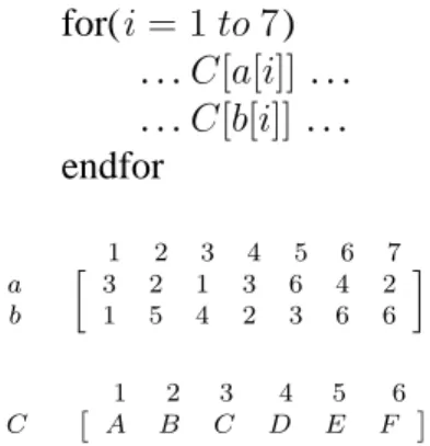
column order. Adding that dynamic reordering algorithms work as inspector-executor method used by Saltz [30]. This corresponds to matrix reordering algorithms that are run before multiplication, they do not run at run-time an it is not necessary because we have the whole matrix that determines computation and data orders. The example code given in Figure 3.1 is the general case of the problem and the code in Figure 3.2 is the special case of computation and data ordering.
Initial studies start with the work of Ding and Kennedy [13]. They propose a dynamic approach for both data and computation reordering. They present consecutive packing (CPACK) where data is ordered when a computaion require it and after then
CHAPTER 3. RELATED WORK 17 for(i = 1 to 7) . . .C[a[i]] . . . . . .C[b[i]] . . . endfor 1 2 3 4 5 6 7 a b » 3 2 1 3 6 4 2 1 5 4 2 3 6 6 – 1 2 3 4 5 6 C ˆ A B C D E F ˜
Figure 3.1: Example for irregular code that are the focus in computation and data ordering problem. C array is accessed through two index arrays a and b. These two
arrays cause indirection so the code shows irregular access patter.
this reordered data no more moved.
Space-filling curves (e.g., Morton, Hilbert) can be used for computation order-ing [20]. They are also used for data orderorder-ing [10] and are shown to be successful in improving locality. Haase et al. [16] use Hilbert space-filling curve to order nonzeros of the matrix A along the curve. They report speedups of up to 50 percent according
to the original CSR scheme.
Hwansoo and Tseng [17] propose an algorithm, Z-SORT, for reordering compu-tations and another algorithm, GPART, for reordering data at run-time in. Z-SORT
algorithm finds a new loop iteration order using Z-curve which is a kind of space-filling curve. GPART orders elements in data array to exploit spatial locality. After data ordered by GPART, Z-SORT finds suitable computation ordering respecting the order found by GPART.
Strout and Hovland [35] give metrics that guide while selecting the best ordering method according to irregularity of applications. They introduce a temporal hyper-graph model for ordering iterations to exploit temporal locality. They also generalize spatial locality graph model to spatial locality hypergraph model to encompass the ap-plications having multiple arrays that are accessed irregularly. Additionally, they pro-pose a modified algorithm like Breadth-First Search for ordering data and iterations simultaneously whereas Breadth-First Search is used for only data ordering in [1].
CHAPTER 3. RELATED WORK 18
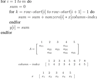
for i = 1 to m do sum = 0
for k = row -start[i] to row -start[i + 1] − 1 do sum = sum + nonzero[i] ∗ x[column-index[k]]
endfor y[i] = sum endfor 1 2 3 4 5 A= 2 4 a11 a14 a22 a23 a24 a32 a34 a35 3 5 1 2 3 4 5 6 7 8 column− index ˆ 1 4 2 3 4 2 4 5 ˜ 1 2 3 4 5 x ˆ x1 x2 x3 x4 x5 ˜
Figure 3.2: Sparse matrix-vecto multiply algorithm based on using the CSR scheme.
x array is the x-vector in the sparse matrix-vector multiplication y ← Ax .
scheme is proposed based on partitioning the rownet hypergraph model of an input sparse matrix A. They achieve spatial locality on x-vector entries by clustering the
columns with similar sparsity pattern. They also exploit temporal locality forx-vector
entries by using zig-zag property of ZZCSR and ZZICSR schemes mentioned in Sec-tion 2.1.2 and 2.1.4 respectively.
White and Sadayappan [39] use graph model for ordering rows and columns us-ing the Metis graph partitioner [22]. Unfortunately they report that they could not gain improvement for reordered matrices compared to original matrices during sparse matrix-vector multiplication.
Pınar and Heath [32] try to permute nonzeros of the matrix A into contiguous
blocks to decrease the number of indirections and they formulate this problem as an instance of the traveling salesman problem.
Beside reordering transformations, locality can be exploited by a cache-aware method called cache blocking like in OSKI framework [37] and in [38]. Our con-tributions in this thesis have both cache-aware and cache-oblivious aspects and they will be presented in Chapters 4 and 5.
Chapter 4
Single Matrix-Vector Multiply
Framework
This is the conventional approach to matrix-vector multiply operation. The y -vector
results are computed simply by multiplying matrixA with x-vector , i.e.,
y ← Ax (4.1)
The objective in this scheme is to reorder the columns and rows of matrix A for
maximizing the exploitation of temporal and spatial locality in accessing x-vector
entries. Recall that temporal locality in accessing y -vector entries is not feasible,
whereas spatial locality is achieved automatically because y -vector results are stored
and processed consecutively. Reordering the rows with similar sparsity pattern nearby increases the possibility of exploiting temporal locality in accessing x-vector entries.
Reordering the columns with similar sparsity pattern nearby increases the possibility of exploiting spatial locality in accessing x-vector entries. This row/column
reorder-ing problem can be considered as a row/column clusterreorder-ing problem and this clusterreorder-ing process can be achieved in two distinct ways: top-down and bottom-up. In this sec-tion, we first propose and discuss a cache-size aware top-down approach based on 1D partitioning of sparse matrix A and then a cache oblivious bottom-up approach
based on hierarchical clustering of rows with similar patterns. Then we propose a col-umn compression scheme as a preprocessing step which makes these two approaches cache-line-size aware.
CHAPTER 4. SINGLE MATRIX-VECTOR MULTIPLY FRAMEWORK 20
4.1
1D Decomposition of Sparse Matrices
We consider a row/column reordering which permutes a given matrix A into a K -way
SB form ASB = P AQ = A11 A1B1 A22 A2B2 . .. ... AKK AKBK = A1 A2 .. . AK . (4.2)
where the CSR data structure associated with each submatrix Ak as follows
Ak= [0 . . . 0 Akk0 . . . 0 AkBk] . (4.3)
Here Akk denotes the k th diagonal block of ASB, whereas AB denotes the column border as follows AB = A1B1 A2B2 .. . AKBK . (4.4)
Each column in the border is called a row-coupling column or simply coupling column. Letλ(cj) denote the number of submatrices that contain at least one nonzero of column
cj of matrix ASB, i.e.,
λ(cj) = |{Ak: cj ∈ Ak}| (4.5)
In this notation, a column cj is coupling column if λ(cj) > 1.
The following theorem gives the guidelines for a “good” A-to-ASB transforma-tion.
Theorem 1 Given a K -way SB form of matrix A such that every submatrix Ak can fit into the cache. Then the number Φ(ASB) of cache misses due to the access of
x-vector entries can be upperbounded as Φ(ASB) ≤
X
cj
λ(cj) (4.6)
CHAPTER 4. SINGLE MATRIX-VECTOR MULTIPLY FRAMEWORK 21
Proof Since each submatrixAk fits into the cache, eachx-vector entry corresponding to a nonzero column of matrix Ak will be loaded to the cache only once during the
yk = Akx multiply, under the full-associativity assumption. Therefore for a column
cj maximum number of cache misses that can occur is bounded above byλ(cj) due to the access of corresponding x-vector entry xj. Thus, the number Φ(ASB) of cache misses due to the access of x-vector entries cannot exceed P
cjλ(cj). Note that this
upperbound also holds for the larger cache-line sizes.
Theorem 1 leads us to a cache-size aware top-down row/column reordering through an A-to-ASB transformation which minimizes the sum Pcjλ(cj) of the λ values of columns. Here, minimizing objective relates to minimizing the cache misses due to temporal locality.
More precisely, under the assumption that there is no empty column, since there has to be at least one cache-miss for each columncj. The column cj brings λ(cj) − 1 extra cache-misses due to temporal locality in the worst case.
Corollary 1 Given a K -way SB form of matrix A such that every submatrix Ak can fit into the cache. Then the numberΦadditional(ASB) of additional cache misses due to the access ofx-vector entries can be upperbounded as
Φadditional(ASB) ≤
X
cj
(λ(cj) − 1) (4.7)
As also discussed in [2], this A-to-ASB transformation problem can be formu-lated as an HP problem using the column-net model of matrix A with a part size
constraint of cache size and partitioning objective of minimizing cutsize according to the connectivity-1 metric definition given in 2.2.
4.2
Hierarchical Clustering
For row/column reordering of sparse matrices, an hierarchical bottom-up approach is also proposed. This idea is inspired from GPART Algorithm proposed by Han and Tseng [17]. A nice property of this approach is being cache-oblivious. Different from
CHAPTER 4. SINGLE MATRIX-VECTOR MULTIPLY FRAMEWORK 22
Han and Tseng, in this approach, hypergraph is used instead of graph. The given sparse matrix is represented as a hypergraph by utilizing the column-net hypergraph model. Thus, the rows are represented by vertices and the columns are represented by nets. The reordering algorithm works in a bottom-up fashion and performs clustering phases as far as it could be. On each clustering pass, the vertices are clustered according to the “heavy net connectivity” metric which is commonly used on coarsening phase of hypergraph partitioning tools. Each cluster is then behaved as a single vertex in the next pass and this forms coarsened hypergraph constituting a hierarchical structure. The coarsening process continues until there exists one vertex left or all vertices are disconnected in the coarsened hypergraph.
The proposed hierarchical clustering algorithm is presented in Algorithm 5. The rows of the sparse matrix is reordered respecting the hierarchy of clustering. That is, the rows are reordered in such a way that the rows corresponding to vertices of a cluster are grouped together. This refers to the idea of clustering the rows with similar sparsity patterns and consequently improves the exploitation of temporal locality. On each clustering pass, first the vertices are sorted in decreasing order of net degrees. Then all vertices are processed respecting to this order. That is, the vertex with more nets is processed before. The intention of “processing the vertex” is either assigning the vertex to a cluster or form a new cluster with another vertex. If the vertex, to be processed, is already clustered, then it is not further assigned to any cluster and the algorithm passes to the next vertex. But if the vertex is not yet clustered, the most attractive cluster is selected. The attractiveness of a cluster is evaluated by heavy net connectivity metric. In this metric, the cluster with largest number of shared nets is most attractive. Note that the other unclustered vertices are considered as one-vertex clusters when we evaluate the attractiveness. Therefore, the processing vertex can either select a cluster or an unclustered vertex as most attractive. If it selects a cluster, the vertex simply joins that cluster. However, if the processing vertex selects an unclustered vertex, than these two vertices form a new cluster. The above-mentioned procedure only reorders the rows of the matrix. The columns are reordered as in CPACK approach in which columns are moved into adjacent locations in the order they are first encountered by a row [13]. Consequently, the overall process presents a simple yet effective algorithm where temporal locality is exploited by reordering rows with similar sparsity patterns nearby by utilizing the hierarchy of clustering and spatial locality is exploited via a post processing.
CHAPTER 4. SINGLE MATRIX-VECTOR MULTIPLY FRAMEWORK 23
4.3
Compression Preprocessing for Spatial Locality
The column-net model exploits temporal locality in the first place. Reordering columns utilizing the information obtained from vertex partition exploits spatial locality. Pro-cess of reordering of columns is not nePro-cessarily to be done if spatial locality is ex-ploited via any method. Such a method is compression of columns. This is a prepro-cessing step in which columns are grouped to form cache-line-sized clusters so that only temporal locality will be considered in further steps. The requirement for taking care of spatial locality disappears in further steps. This approach can be used as a preprocessing step of any row reordering method.
The columns with similar sparsity pattern are clustered to form cache-line-sized clusters. If a cluster cannot reach size of cache line, then they are left single. Clus-tering process is performed via successive matchings of columns. All columns are singleton clusters at the beginning. Clusters are processed in random order. Each cluster selects the most attractive unprocessed cluster. The cluster that shares maxi-mum number of rows with the selector cluster is most attractive. After every cluster selects another cluster, one level ends and another level starts so number of levels is
log2cachelinesize. Each final cluster corresponds to a new column. This matrix can be further processed for temporal locality. After this process, it is decompressed and passed to matrix-vector multiply operation.
Consequently, this preprocessing approach makes any reordering method cache-line-size aware.
CHAPTER 4. SINGLE MATRIX-VECTOR MULTIPLY FRAMEWORK 24
Algorithm 4 Hypergraph Based Bottom-up Reordering HPART
Require: Hypergraph H = (U, N ), Tree level t
1: if| U| = 1 or nodes of H are disconnected then
2: return t
3: end if
4: Hcoarsen← HCLU ST ER(H)
5: tupper.lower← t
6: return HPART(Hcoarsen, t)
Algorithm 5 Hypergraph Based Clustering HCLUSTER
Require: Hypergraph H = (U, N )
1: C ← ∅
2: for each node u∈ U do
3: selected[u] ← F ALSE
4: C ← C ∪ {{u}}
5: end for
6: for each node u∈ U in decreasing order of number of nets do
7: if selected[u] = F ALSE then
8: C ← C − {{u}} 9: max← 0
10: for each cluster c∈ C do
11: S ← ∅
12: for each node v∈ c do
13: S ← S ∪ N ets[v] 14: end for 15: S ← S ∩ N ets[u] 16: if max <|S| then 17: max← |S| 18: maxc← c 19: end if 20: end for 21: if max >0 then 22: C ← C − {maxc} 23: if |maxc| = 1 then
24: selected[v ] ← T RU E , where maxc = {v}
25: end if 26: c← maxc ∪ {u} 27: C ← C ∪ c 28: end if 29: end if 30: end for
Chapter 5
Multiple Submatrix-Vector Multiplies
Framework
In this framework, we assume that the nonzeros of matrixA are partitioned arbitrarily
amongK submatrices such that each submatrix Ak contains a mutually disjoint subset of nonzeros. Then matrix A can be written as
A = A1+ A2+ · · · + Ak (5.1)
Note that this partitioning is not necessarily row disjoint or column disjoint. That is, the nonzeros of a given column of matrix A might be shared by multiple
submatri-ces. Similarly, the nonzeros of a given row of matrix A might be shared by multiple
submatrices. In this framework, y ← Ax can be computed as
fork ← 1 to K (5.2)
y ← y + Akx
The partitioning of matrix A into submatrices Ak should be done in such a way that the temporal and spatial locality of individual submatrix-vector multiplications are ex-ploited in order to minimize cache misses during an individual submatrix-vector mul-tiplication. This goal is similar as Single Matrix-Vector Multiply framework discussed in Chapter 4. On the contrary, this framework requires partitioning of the matrix A
into submatrices whereas previous framework uses the method of reordering rows and columns. We discuss pros and cons of this framework according to the conventional
CHAPTER 5. MULTIPLE SUBMATRIX-VECTOR MULTIPLIES FRAMEWORK26
framework y ← Ax in Section 5.1. In Section 5.2, we also show that partitioning
the matrix A into submatrices can be performed by 2D-partitioning of fine-grain
hy-pergraph model. The order of individual submatrix-vector multiply operations is also important to exploit temporal locality. We state this ordering problem as an instance of traveling salesman problem in Section 5.3.
5.1
Pros and Cons compared to Conventional
Frame-work
Since a global row and column ordering is assumed in Equation 5.3, submatrices are likely to contain empty rows. Hence, each individual sparse submatrix-vector multiply operation y → y + Akx is performed using the ICSR scheme. As seen Algorithm 6, individual submatrix-vector multiply results are accumulated in the output vector y on
the fly in order to avoid additional write operations.
Algorithm 6 Multiple Sparse Submatrix-Vector Multiplications using ICSR scheme
Require: nonzerok, column -diffk and row -jumpk arrays of a mk by nk sparse subma-trix Ak where k = 1, 2 . . . K , K is total number of submatrices, number of nonzeros nnzk in matrix Ak,
a dense input vector x
1: for k← 1 to K do 2: i← row -jumpk[0] 3: j← column-diffk[0] 4: t← 0 5: r← 1 6: tmp← 0 7: while t < nnzk do 8: tmp← tmp + nonzerok[t] ∗ x[j] 9: t← t + 1 10: j← j + column-diffk[t] 11: if j ≥ n then 12: y[i] ← tmp 13: tmp← 0 14: j← j − nk 15: i← i + row -jumpk[r] 16: r← r + 1 17: end if 18: end while 19: end for 20: return y
CHAPTER 5. MULTIPLE SUBMATRIX-VECTOR MULTIPLIES FRAMEWORK27
Note that the conventional single matrix-vector multiply framework can be consid-ered as a special case in which submatrices are also restricted to be row disjoint. Thus, this framework brings an additional flexibility for exploiting the temporal and spa-tial locality. Clustering A-matrix rows/subrows with similar sparsity pattern into the
same submatrices increases the possibility of exploiting temporal locality in accessing
x-vector entries. Clustering A-matrix columns/subcolumns with similar sparsity
pat-tern into the same submatrices increases the possibility of exploiting spatial locality in accessingx-vector entries as well as temporal locality in accessing y -vector entries.
However, this additional flexibility comes at a cost of disturbing the following lo-cality compared to conventional approach. There is some disturbance in the spatial locality in accessing the nonzeros of the A-matrix due to the division of three arrays
associated with nonzeros into K parts. However, this disturbance in spatial locality is
negligible since elements of each of the three arrays are stored and accessed consecu-tively during each submatrix vector multiply operation. That is, at most3(K −1) extra
cache misses occur compared to the conventional y ← Ax scheme due to the
distur-bance of spatial locality in accessing the nonzeros ofA-matrix . Furthermore, multiple
read/writes of the submatrix-vector multiply results might bring some disadvantages compared to conventional single matrix-vector multiply. These multiple read/writes disturb the spatial locality of accessing y -vector entries as well as introducing a
tem-poral locality exploitation problem in y -vector entries.
Our problem here, can be defined as the matrix-to-submatrix partitioning prob-lem. As a solution, the following theorem gives the guidelines for a “good” matrix-to-submatrix partitioning:
Theorem 2 Consider a partition Π(A) of matrix A into K nonzero-disjoint
subma-trices A1, A2, . . . , AK. Let λ(r
i) denote the number of submatrices that contain at least one nonzero of row ri of matrix A, i.e., λ(ri) = |{Ak : ri ∈ Ak}|. Similarly let
λ(cj) denote the number of submatrices that contain at least one nonzero of column
cj of matrix A, i.e., λ(cj) = |{Ak : cj ∈ Ak}|.Let q denote the maximum number of caches that a submatrix can fit into. Then the number Φ(Π(A)) of cache misses due
to the access of x-vector and y -vector entries can be upperbounded as
Φ(Π(A)) ≤X ri λ(ri) + q X cj λ(cj) (5.3)
CHAPTER 5. MULTIPLE SUBMATRIX-VECTOR MULTIPLIES FRAMEWORK28
if cache is assumed to be fully-associative.
Proof Consider the case that the line size is equal to the x/y -vector entry size. For
each submatrix Ak, each y -vector result of Ak is written only once to the memory. For the sake of simplicity, we referΦ(Π(A)) as Φ. Let Φx andΦy respectively denote the number of cache misses due to the access of x-vector and y -vector entries for Π(A). Then,
Φ = Φx+ Φy (5.4)
The number of cache misses due to the access of yi is at most λ(ri) which happens when no cache-reuse occurs in accessing toyi, that is,
Φy ≤
X
ri
λ(ri). (5.5)
Let qk denote the minimum number of caches that submatrix Ak can fit into. Since full-associativity is assumed, for each submatrix Ak, each x-vector entry of Ak is accessed at most qk times. Therefore, the number of cache misses due to the access of
xj is at most qk for each submatrix Ak that xj is needed to be accessed. Then,
Φx ≤ X cj X k:cj∈Ak qk (5.6) ≤ X cj X k:cj∈Ak q (5.7) = qX cj X k:cj∈Ak 1 (5.8) = qX cj λ(cj) (5.9)
Equation 5.4, Equation 5.5 and Equation 5.9 together yield to Equation 5.3. Extending the line size can only increase the reuse and accordingly decrease the cache-miss. Therefore, Equation 5.3 still holds for larger line sizes.
Corollary 2 When all submatrices fit into the cache then the number Φ(Π(A)) of
cache misses due to the access ofx-vector and y -vector entries can be upperbounded
as Φ(Π(A)) ≤X ri λ(ri) + X cj λ(cj) (5.10)
These theorems give exact upper bounds for when temporal reuse is exploited at the utmost degree via fully-associativity.
CHAPTER 5. MULTIPLE SUBMATRIX-VECTOR MULTIPLIES FRAMEWORK29
5.2
2D Decomposition of Sparse Matrices
The aim is to partition the given sparse matrixA into K nonzero-disjoint submatrices.
Corollary 2 leads us to a cache-size aware top-down matrix-to-submatrix partitioning which minimizes the sumP
riλ(ri)+
P
cjλ(cj) of λ values of rows and columns such
that the storage of each submatrix-vector multiply fits into the cache. Here, minimizing objective relates to minimizing the cache misses due to temporal locality.
More precisely, under the assumption that there is no empty column, since there has to be at least one cache-miss for each rowri and each column cj. Thus the rowri and the column cj, respectively, bring λ(ri) − 1 and λ(cj) − 1 extra cache-misses due to temporal locality in the worst case.
Corollary 3 Given a K -way matrix-to-submatrix partition Π(A) of matrix A such
that every submatrix Ak can fit into the cache. Then the number Φ
additional(Π(A)) of additional cache misses due to the access of x-vector and y -vector entries can be
upperbounded as Φadditional(Π(A)) ≤ X ri (λ(ri) − 1) + X cj (λ(cj) − 1) (5.11)
The matrix-to-submatrix partition problem can be formulated as an HP problem using the row-column-net model of matrix A with a part size constraint of cache size
and partitioning objective of minimizing cutsize according to the connectivity-1 metric definition given in Equation 2.2.
5.3
Ordering Submatrix-Vector Multiplies
The partitioning of matrix A into submatrices Ak should be done in such a way that the temporal and spatial locality of individual submatrix-vector multiplications are ex-ploited in order to minimize cache misses during an individual submatrix-vector multi-plication. When all the multiplications are considered, data reuse between two consec-utive submatrix-vector multiplications must be maximized to exploit temporal locality. We give an exact lower bound for the cache misses due to the access ofx-vector and y -vector entries for a given order of submatrices.
CHAPTER 5. MULTIPLE SUBMATRIX-VECTOR MULTIPLIES FRAMEWORK30
Theorem 3 Consider a partition ˆΠ(A) of matrix A into K nonzero-disjoint
subma-trices A1, A2, . . . , AK with a given ordering of the submatrices. Let γ(r
i) and γ(cj), denote the number of submatrix-subchains in which all submatrices contain at least one nonzero of row ri and column cj, respectively. Letw denote the line size in terms of a unitx/y -vector entry. If no submatrix Ak can fit into one cache, then the number
Φ( ˆΠ(A)) of cache misses due to the access of x-vector and y -vector entries can be
lowerbounded as Φ( ˆΠ(A)) ≥ P riγ(ri) + P cjγ(cj) w (5.12)
Proof We will give the proof only for the columns, since a similar proof applies for the rows; then total number of cache misses can be written as sum of cache misses due to access ofy -vector entries and x-vector entries and can be formulated as
Φ( ˆΠ(A)) = Φr( ˆΠ(A)) + Φc( ˆΠ(A)) (5.13) Consider a column cj of matrix A. Then there exists γ(cj) submatrix-subchains for columncj. Since no submatrixAk can fit into one cache, it is guaranteed that there will be no cache-reuse of column cj between two different submatrix-subchains including
cj. Therefore, at least γ(cj) cache misses will occur for each column cj which yields that the number Φc( ˆΠ(A)) of cache misses due to the access of x-vector entries is greater than or equal to P
ri
P
cjγ(cj) in the case of unit cache-line-size, i.e., w =
1. Since the number of cache-misses can maximally decrease w -fold, the number Φc( ˆΠ(A)) of cache misses due to the access of x-vector entries is greater than or equal to
P
cjγ(cj)
w .
Theorem 4 Consider the TSP Instance (G = (V, E), w ), where vertex set V
de-notes the K submatrices. There exists an edge eij in E if and only if there exists at least one row or column shared between submatrices Ai and Aj. The weight of edge wij denotes the sum of the number of shared rows and the number of shared columns between submatrices Ai and Aj. Then, finding an order of V which maxi-mizes the path weight corresponds to finding an order of submatrices which minimaxi-mizes
P
riγ(ri) +
P
CHAPTER 5. MULTIPLE SUBMATRIX-VECTOR MULTIPLIES FRAMEWORK31 Proof X ri γ(ri) + X cj γ(cj) = X ri (|Ai1 ∩ {ri}| + K X k=2 |(Aik− Aik−1) ∩ {ri}|) + X cj (|Ai1 ∩ {cj}| + K X k=2 |(Aik− Aik−1) ∩ {cj}|) = |Ai1| + K X k=2 |(Aik − Aik−1)| = |Ai1| + K X k=2 |(Aik − (Aik∩ Aik−1))| = |Ai1| + K X k=2 (|Aik| − |Aik ∩ Aik−1|) = K X k=1 |Aik| − K X k=2 |Aik∩ Aik−1| = K X k=1 |Aik| − K X k=2 wik,ik−1
In the above formulation, Aik is used to denote the k th submatrix in the order of
submatrices and Aik is also used to denote the set of rows and columns that belong
to the submatrix Aik. The maximum value of
PK
k=2wik,ik−1 will yield the minimum
value ofP
riγ(ri)+
P
cjγ(cj). Then, finding an order of V which maximizes the path
weightPK
k=2wik,ik−1 corresponds to finding an order of submatrices which minimizes
P
riγ(ri) +
P
cjγ(cj).
According to Theorem 4, the lower bound P
riγ(ri) +
P
cjγ(cj) corresponds to
Chapter 6
Experimental Results
Throughout the previous chapters, we investigate ways of exploiting data locality by reordering/partitioning a sparse matrix A. In this chapter, we show the improvements
gained by the proposed models and frameworks. A cache simulator is used to show these improvements. The existing state-of-the-art models such as row-net model [40] and BFS-based algorithm [1] are also tested.
6.1
Experimental Setup
The two contributed frameworks and underlying models are based on decreasing cache misses incurred by x-vector and y -vector entries so using a cache simulator will
make the improvement obtained by our contributions more clear. One must pay more attention to sum of cache misses caused by x-vector and y -vector entries to see the
proof of our proposed concepts.
All simulation results are normalized according to the number of cache misses for original, unprocessed matrices. The cache miss ratio is 1.00 if the number of cache misses does not change. If number of cache misses is decreased when a method ap-plied, the ratio is smaller than 1.00. Similarly, if number of cache misses is increased when a method applied, the ratio is greater than 1.00. The used normalization equation
CHAPTER 6. EXPERIMENTAL RESULTS 33
is as follows:
ratio = missreordered missoriginal
(6.1)
The data type used in storage of matrices is double precision floating-point number which has size of 8 bytes on the test platform. Only the index arrays use integers which have size of 4 bytes.
6.1.1
Platform
The experiments of using original matrices and reordered matrices in the single matrix-vector multiply framework are performed on a cache simulator also used in [40].The experiments related with the multiple matrix-vector multiplies framework are also per-formed on the cache simulator.
Simulation results of experiments are given for when cache line size is size of 8 doubles, cache size is 32KB and set-associativity is 8. This configuration is taken from [40]. Some of results are given for when cache line size of 1 double and number of cache lines is one eighth of original cache line number so that cache size is still 32KB. The aim is to show only the effect of temporal locality clearly because spatial locality for x and y vectors cannot exist when only 1 double is retrieved when a cache miss
occurs.
6.1.2
Data Sets
The proposed frameworks are tested and validated on numerous matrices collected from The University of Florida Sparse Matrix Collection [36]. General properties of these matrices can be seen Table 6.1.
The columns can be explained as follows:
1. #Rows : number of rows
2. #Cols : number of columns