RELAXATION MAPPING IN
MAGNETIC PARTICLE IMAGING
a thesis submitted to
the graduate school of engineering and science
of bilkent university
in partial fulfillment of the requirements for
the degree of
master of science
in
electrical and electronics engineering
By
Yavuz Muslu
January 2018
RELAXATION MAPPING IN MAGNETIC PARTICLE IMAGING By Yavuz Muslu
January 2018
We certify that we have read this thesis and that in our opinion it is fully adequate, in scope and in quality, as a thesis for the degree of Master of Science.
Emine ¨Ulk¨u Sarıta¸s C¸ ukur (Advisor)
Ergin Atalar
Nevzat G¨uneri Gen¸cer
Approved for the Graduate School of Engineering and Science:
Ezhan Kara¸san
ABSTRACT
RELAXATION MAPPING IN
MAGNETIC PARTICLE IMAGING
Yavuz Muslu
M.S. in Electrical and Electronics Engineering Advisor: Emine ¨Ulk¨u Sarıta¸s C¸ ukur
January 2018
Magnetic Particle Imaging (MPI) is a novel biomedical imaging modality that shows great potential in terms of sensitivity, resolution, and contrast. Since its first introduction in 2005, several applications of MPI have already been de-monstrated such as angiography, stem cell tracking, and cancer imaging. Recently, multi-color MPI techniques have been proposed to increase the functionality of MPI, where different nanoparticles are distinguished according to the differences in their responses to oscillating magnetic fields. These methods can also be exten-ded to probe environmental factors such as viscosity and temperature, proviexten-ded that the responses of different nanoparticles or nanoparticles in different environ-ments are pre-calibrated. This thesis proposes a new multi-color MPI technique that does not require a calibration phase. This new technique directly estimates the relaxation time constants of nanoparticles to distinguish nanoparticle types and environmental factors from the MPI signal, and generates a multi-color re-laxation map. The validity of the proposed technique is confirmed through an extensive experimental work with an in-house Magnetic Particle Spectrometer (MPS) at 10.8 kHz and an in-house MPI scanner at 9.7 kHz drive field fre-quencies, successfully distinguishing different nanoparticle types. The proposed calibration-free multi-color MPI technique is a promising method for future func-tional imaging applications of MPI.
Keywords: Magnetic Particle Imaging, Multi-Color MPI, Magnetic Nanoparticle Relaxation, Direct Estimation, Mirror Symmtery.
¨
OZET
MANYET˙IK PARC
¸ ACIK G ¨
OR ¨
UNT ¨
ULEMEDE
RELAKSASYON HAR˙ITALAMA
Yavuz Muslu
Elektrik Elektronik M¨uhendisli˘gi, Y¨uksek Lisans Tez Danı¸smanı: Emine ¨Ulk¨u Sarıta¸s C¸ ukur
Ocak 2018
Manyetik Par¸cacık G¨or¨unt¨uleme (MPG) duyarlılık, ¸c¨oz¨un¨url¨uk ve kontrast a¸cısından y¨uksek potansiyel g¨osteren yeni bir biyomedikal g¨or¨unt¨uleme y¨ ontemi-dir. 2005’teki ilk sunulu¸sundan bu yana, MPG’nin anjiyografi, k¨ok h¨ucre takibi ve kanser g¨or¨unt¨uleme gibi bir¸cok uygulaması deneysel olarak g¨osterilmi¸stir. Yakın zamanda renkli MPG teknikleri ¨onerilmi¸s ve manyetik alan de˘gi¸simlerine farklı tepkiler veren nanopar¸cacıkların ayırt edilmesi sa˘glanmı¸stır. Bu teknikler sıcaklık ve viskozite gibi ortam ¨ozelliklerini ayırt edecek ¸sekilde geni¸sletilebilmektedir, ama bunun i¸cin farklı nanopar¸cacık tepkilerinin kalibrasyonunun ¨onceden yapılması ge-rekmektedir. Bu tezde kalibrasyon gerektirmeyen yeni bir renkli MPG tekni˘gi ¨ one-rilmektedir. Bu teknik, nanopar¸cacıkların relaksasyon zaman sabitini do˘grudan MPG sinyalinden hesaplayıp, farklı nanopar¸cıkları ve ortam ¨ozelliklerini ayırt etmektedir. ¨Onerilen teknik, ¨ozel olarak tasarlanmı¸s bir manyetik par¸cacık spekt-rometre (MPS) d¨uzene˘gi ile 10.8 kHz frekansta ve ¨ozel olarak tasarlanmı¸s bir MPG tarayıcısında 9.7 kHz frekansta deneyler ile g¨osterilmi¸stir. Bu deneylerde 3 farklı nanopar¸cacık tipinin ba¸sarıyla ayırt edilmesi sa˘glanmı¸stır. ¨Onerilen ka-librasyonsuz renkli MPG tekni˘gi, MPG’nin gelecekteki fonksiyonel g¨or¨unt¨uleme uygulamaları i¸cin umut veren bir y¨ontemdir.
Anahtar s¨ozc¨ukler : Manyetik Par¸cacık G¨or¨unt¨uleme, Renkli MPG, Manyetik Na-nopar¸cacık Relaksasyonu.
Acknowledgement
Completing my undergraduate education brought up more questions than it ans-wered, in terms of the career path that I wanted to choose. Although I had certain academic interests and subjects that I found closer to me, it was not until the gra-duate admissions that I realized my passion for biomedical engineering. For that, I feel very fortunate to have met my master’s degree advisor, Emine ¨Ulk¨u Sarıta¸s, before the graduate school admissions. During the admission interviews and she took the time to explain her research field and answered my questions patiently. Because of her understanding and thoughtful attitude during the interviews, I felt very comfortable taking the graduate student position under her supervision. She cares about her students immensely, spares no effort to guide them through their research, and shares her knowledge and experience very generously. She wel-comes questions anytime her students need help but motivates them to become independent researchers. She is the most thoughtful, selfless and kindest advisor anyone can hope for, and it was a privilege to have worked with her during my graduate studies.
I would like to thank Ergin Atalar and Nevzat G¨uneri Gen¸cer for taking the time to be in my master’s degree thesis committee. Their feedbacks and discussi-ons were very valuable, and will surely affect the future of this study positively.
I would like to thank the following funding agencies for supporting the work in this thesis: the Scientific and Technological Research Council of Turkey through TUBITAK Grants 114E167 and 115E677, the European Commission through FP7 Marie Curie Career Integration Grant (PCIG13-GA-2013-618834), the Turkish Academy of Sciences through TUBA-GEBIP 2015 program, and the BAGEP Award of the Science Academy.
I would also like to thank my research group mates, who are also close fri-ends: Alper ¨Ozaslan, C¸ a˘gla Deniz Bahadır, Damla Sarıca, Ecem Bozkurt, Mus-tafa ¨Utk¨ur, ¨Omer Burak Demirel, Sevgi G¨ok¸ce Kafalı, and Toygan Kılı¸c. They were always kind, helpful and a lot of fun. Mustafa and Burak spent lots of time
vi
with me in the lab trying to figure out what was wrong with the experiment setup, which, in the end, provided some of the funniest and most fulfilling memo-ries of my graduate life. Although we could not realize Burak’s minimalist design plans for our setup, which included significant amount of woodwork, it was really fun to work with them. Whenever I needed a break from the research, Toygan and Alper were always there for me to either distract with my nonsense or start some serious discussions about their research. C¸ a˘gla kept my ties with art and literature alive with her brilliant suggestions on classical music, plays and books. Going to the theater with her always gave me a peace of mind even when there were a lot of work to be completed in the lab.
I would also like to thank my cubicle mates, or as we would call ourselves “the champion cubicle”: Akbar Alipour, Koray Ertan, Cemre Arıy¨urek, Mustafa
¨
Utk¨ur, and Sevgi G¨ok¸ce Kafalı. Their sense of humor picked me up whenever I felt tired or frustrated. Koray provided some interesting and enjoyable discussions with his funny but spot on takes on life. Sevgi, having gone through similar stages in our graduate studies, was always very understanding and helpful. It was also very motivating to set ourselves some serious challenges on the completion of our research projects, which definitely helped all of us. Akbar Alipour never failed to make us feel guilty with his organized and extremely healthy life style. Efe and
¨
Ozg¨ur made our office a more fun place to be around, which helped a lot when I needed to work in the evenings or weekends.
I would like to thank Se¸ckin and Barı¸s for helping me throughout my graduate studies. Whenever I wanted to improve my knowledge on politics or economics, or clear my head with some funny anecdotes, I could count on them to be there for me. I enjoyed our discussions on the investments that we never had and the money that we never made via those investments. Although our ideas conflicted at times, we have learned a lot from each other.
Finally, I would like to thank my family for their endless support throughout my graduate studies. They were always by my side whenever I needed help. It is because of their support and trust in me, that I found the motivation to keep moving forward in difficult times. I would like to thank, especially my brother
vii
Kerem. Due to the similar career paths we select, I could always share the diffi-culties that I face and expect a sound suggestion from him. After providing one, he would never miss the opportunity to make fun of me a little bit just to remind me to take the life easier. I would not be able to complete my thesis without their help and support, that is why I will always be grateful to them.
Yavuz Muslu January 2018
Contents
1 Introduction 1
2 Background and Theory 4
2.1 Magnetic Particle Imaging Physics . . . 4
2.1.1 Spatial Encoding . . . 4
2.1.2 1D MPI Signal Equation . . . 5
2.1.3 SPIO Relaxation . . . 8
2.2 Image Reconstruction Methods . . . 9
2.2.1 System Function Reconstruction . . . 9
2.2.2 X-space Reconstruction . . . 10
2.3 Multi-color Magnetic Particle Imaging . . . 12
3 Direct Relaxation Time Constant Estimation 14 3.1 Theory . . . 14
CONTENTS ix
3.2 Simultaneous Hardware Delay and Relaxation Time Constant
Es-timation . . . 18
3.3 Magnetic Particle Spectrometer Experiments . . . 19
3.3.1 MPS Setup . . . 19
3.3.2 Sample Preparation . . . 21
3.4 Results . . . 21
4 Calibration-Free Multi-Color MPI 24 4.1 Algorithm . . . 24
4.2 1D and 2D Simulations . . . 28
4.2.1 Methods . . . 28
4.2.2 Results . . . 29
4.3 Magnetic Particle Imaging Experiments . . . 32
4.3.1 MPI Scanner . . . 32
4.3.2 Sample Preparation . . . 34
4.3.3 Results . . . 35
5 Discussion 39 5.1 Effects of SPIO Types and Imaging Parameters . . . 40
5.2 Resolution of the Relaxation Map . . . 40
CONTENTS x
5.4 Towards True Quantitative MPI . . . 42 5.5 Extensions to 2D/3D Excitation and FFL Scanners . . . 42
6 Conclusion 44
A Relaxation Time Constant of a Homogeneous Mixture 52 B Effects of pFOV overlap on the Relaxation Map 54
C Local Minima Analysis 56
C.1 The Effects of Hardware Delays . . . 56 C.2 Uniqueness of Local Minimum . . . 58
List of Figures
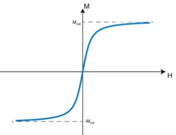
2.1 Nonlinear magnetization curve of SPIOs. Horizontal axis (H) shows the external magnetic field, vertical axis (M) shows the SPIO magnetization. Msat denotes the saturation magnetization of SPIOs. 5
2.2 (a) Topology of an MPI scanner, where black circles denote selec-tion field coils. Here, blue arrows denote the magnetic field lines and their directions. Orange dot denotes the FFP, while yellow dot denotes a region where the SPIOs are saturated by the selec-tion field. (b) Comparison of signals acquired from SPIOs that are unsaturated (orange) and saturated (yellow) by the selection field. Here, orange and yellow regions experience the same sinu-soidal drive field, with a different selection field component. When particles are not saturated, they induce a signal on the receive coil (orange plots). When the particles are saturated, they cannot re-act to the sinusoidal drive field and cannot induce a signal on the receive coil (yellow plots). . . 6
LIST OF FIGURES xii
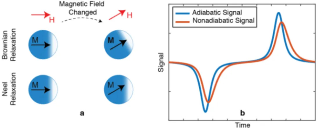
2.3 (a) Illustration of Brownian and Neel relaxations. Initially mag-netic moments of the SPIOs are aligned with the horizontal ex-ternal magnetic field. When exex-ternal magnetic field is rotated, SPIOs physically rotate to align their magnetization via the Brow-nian relaxation process, and/or SPIOs change the direction of their magnetic moments internally via the Neel relaxation process. (b) MPI signal with and without relaxation. Here adiabatic signal de-notes the MPI signal without relaxation, and nonadiabatic signal denotes the MPI signal with relaxation. Due to the relaxation ef-fects, the MPI signal lags (peak of the signal shifts in time), widens, and loses SNR (peak amplitude of the signal decreases). . . 8 2.4 Illustration of calibration measurement for SFR. Here, calibration
for one pixel location is illustrated. Red dot denotes a point source that is used for calibration. Blue curve denotes the FFP trajectory that scans the entire FOV. Once the signal is acquired with this FFP trajectory, Fourier transform of this measurement is recorded to the a column of the system matrix. Each column in the sys-tem matrix corresponds to a calibration measurement from one pixel. Overall calibration procedure includes the calibration mea-surements for every pixel in the FOV. . . 10 2.5 Illustration of X-space Reconstruction. (a) An example circular
SPIO distribution. (b) Multidimensional PSF of the MPI system. (c) Image obtained with the x-space reconstruction. The resulting image shows the SPIO distribution blurred by the PSF of the system. 11
LIST OF FIGURES xiii
3.1 The mirror symmetry of the adiabatic MPI signal and how the relaxation effects break that mirror symmetry. (a) A ramp-shaped nanoparticle density. (b) The corresponding ideal MPI image ob-tained by the convolution of nanoparticle density and the point spread function. (c) Adiabatic vs. non-adiabatic MPI signals for a ramp-shaped nanoparticle density. Here, one full periods of the signals are shown (i.e., the signals from both the negative and posi-tive cycles). (d) In the adiabatic case, due to the repetiposi-tive nature of applied sinusoidal drive field, positive and mirrored negative signals match perfectly. This phenomenon is referred as ”mirror symmetry”. (e) The relaxation effect causes an asymmetric blur-ring of the negative and positive signals, which in turn breaks the mirror symmetry. . . 16 3.2 The proposed method: direct relaxation time constant estimation.
(a) The mirror symmetry between the positive and negative sig-nals is broken due to relaxation. The proposed method estimated ˆ
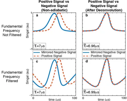
τ = 6.96 µs, where τ = 7 µs in theory. (b) MPI signal is then de-convolved with the estimated relaxation kernel using ˆτ = 6.96 µs, which recovers the underlying mirror symmetry. Here, (a, b) demonstrate the case where the fundamental frequency is kept in-tact in simulations, and (c, d) demonstrate the case after direct feedthrough filtering that removes the fundamental frequency. In the latter case, the estimation resulted in ˆτ = 6.99 µs. . . 17
LIST OF FIGURES xiv
3.3 Experimental relaxation time constant estimation algorithm. (a) A time point tedge is chosen to mark the time when positive scan
finishes and negative scan starts. Then, τ is estimated for different tedge values chosen from [0, T/2) interval. The MSE between the
deconvolved positive and mirrored negative signals are computed for each case. (b) The MSE values are compared, and the (τ, tedge)
pair that minimizes MSE is chosen as the solution. For this exam-ple, the result is ˆτ = 3.51 µs. Here, the black arrows show the flow of the algorithm, while blue arrows show a visual demonstration of each step. . . 20 3.4 Experimental demonstration in the MPS setup. (a) Picture of our
in-house MPS setup, showing the drive and receive coils placed co-axially. (b) Signal acquired from Nanomag-MIP (blue) and Viv-oTrax (orange) SPIOs, and their homogeneous mixture (yellow). The Nanomag-MIP and VivoTrax SPIOs yielded ˆτ = 3.28 µs and ˆ
τ = 4.46 µs, respectively. . . 22 3.5 Experimental demonstration of the homogeneous mixture case in
the MPS setup. (a) Picture of our in-house MPS setup, show-ing the drive and receive coils placed co-axially. (b) Signal ac-quired from Nanomag-MIP (blue) and VivoTrax (orange) SPIOs, and their homogeneous mixture (yellow). The Nanomag-MIP and VivoTrax SPIOs yielded ˆτ = 3.28 µs and ˆτ = 4.46 µs, respectively. The homogeneous mixture gave ˆτ = 3.89 µs, closely matching the expected value of 3.87 µs based on the average of the Nanomag-MIP and VivoTrax relaxation times. . . 23
LIST OF FIGURES xv
4.1 The proposed relaxation mapping algorithm. (a) The simulated particle distributions for two different SPIO types, which overlap in a small region in 1D space. (b) The x-space reconstructed MPI image. (c) Signal RMS values for each pFOV. (d) The initial re-laxation time constant estimations are plotted as a histogram, and (e) the histogram is corrected by eliminating low SNR regions and overestimations (i.e., an upper threshold set at T/4). (f) A k-means clustering detects two main clusters (shown in orange and red). (g) These regions are highlighted in the initial τ map. (h) The inhomogeneous nanoparticle mixture region is detected, and (i) the final τ map is achieved via modeling the transition using a smooth sigmoid curve and setting low pixel intensity regions to zero. Note the change in y-axis scaling from (h) to (i). . . 26 4.2 Results of 1D simulations for three different cases for SNR=5,
with-out signal averaging. Left column (a, d, g) demonstrates the spa-tial distributions for different SPIOs with relaxation time constants ranging between 1-5 µs. Middle column (b, e, h) demonstrates the corresponding x-space MPI images. Right column (c, f, i) demon-strates the relaxation maps reconstructed with the proposed algo-rithm. The mean estimation error is well below 3% for (c), and is around 7% for (i) due to reduced distances between the different SPIO distributions. . . 30
LIST OF FIGURES xvi
4.3 Results of 3D simulations, for SNR=5. (a) A distribution with homogeneous mixtures of 2.9 µs and 1.1 µs SPIOs in different concentrations. Each mixture is labeled with a number from 1 to 9, with concentrations of 2.9 µs SPIO in each mixture given as (100, 87.5, 75, 62.5, 50, 37.5, 25, 12.5, 0)%, respectively. (b) The x-space MPI image, and (c) the color overlay of the multi-color relaxation map and the MPI image. (d) The estimated time constants vs. relative concentrations of the two SPIOs. Here, the error bars denote the standard deviations for each ROI, and the red dashed curve is the fitted line (with R2 = 0.9921). FOV size
is 9x9 cm2. The Euclidean distance between neighboring samples is 1.7 cm. . . 31 4.4 An overview of the MPI scanner and the experimental setup. (a)
The entire imaging system is controlled through MATLAB, via a custom MPI imaging toolbox. First, robot position is adjusted to place the phantom at the desired location. Second, a drive field at 9.7 kHz is applied through the transmit chain, and the nanoparticle signal is simultaneously acquired through the receive chain. (b-c) Front and side views of our in-house MPI scanner. The phantoms imaged in (d) the 1D experiment and (e) the 2D experiment. . . . 33 4.5 Calibration-free multi-color MPI results in 1D. The imaging
ex-periment was conducted at 9.7 kHz and 15 mT-peak drive field, using three different nanoparticles. (a) 1D reconstructed x-space MPI image, and (b) the corresponding multi-color relaxation map. (c) The color overlay of the MPI image and the multi-color map shows that the nanoparticles can be clearly distinguished based on their relaxation responses. (d) A photo of the imaged phantom with three tubes containing Perimag, VivoTrax and Nanomag-MIP SPIOs from left to right, separated at 8mm distances. . . 36
LIST OF FIGURES xvii
4.6 Calibration-free multi-color MPI results in 2D. The imaging ex-periment was conducted at 9.7 kHz and 15 mT-peak drive field, using Nanomag-MIP and VivoTrax SPIOs, and their homogeneous mixture. (a) The reconstructed x-space MPI image and (b) the corresponding multi-color relaxation map. (c) The color overlay of the MPI image and the multi-color map shows that the two nanoparticles and their homogeneous mixture can be clearly dis-tinguished in 2D, solely based on their relaxation responses. The mixture yields a τ value that closely matches the signal-weighted average of the τ values from Nanomag-MIP and VivoTrax. (d) A photo of the imaged phantom with three tubes containing Vivo-Trax, the homogeneous mixture, and Nanomag-MIP from left to right, separated at 15 mm distances. . . 38 B.1 Results of the resolution study. (a) Nanoparticle distributions with
two distinct τ values. Each row demonstrates a simulation result for a different pFOV overlap (e.g. 90%, 80%, 60% and 40%). For the first two rows, the resolution of the MPI system is larger than the spatial overlap (or pixel size) of the pFOVs. As such, the resolution of the relaxation map is equal to the resolution of the MPI system. For the last two rows, the pixel size of the relaxation map is larger than the resolution of the MPI system. Accordingly, the resolution of the relaxation map is equal to the pixel size of the relaxation map. . . 55 C.1 Simulation results for the uniqueness of the local minimum of Eq.
3.9. Here, the logarithm of the MSE between the positive and mir-rored negative signals after the deconvolution is calculated across different (τ, tedge) pairs. The vertical axes show the range of tedge,
while the horizontal axes show the range of τ values. The simula-tion results for the actual pairs of (a) (τ, tedge)actual= (1 µs, 0), (b)
(τ, tedge)actual = (3 µs, 0), and (c) (τ, tedge)actual = (5 µs, 0). The
LIST OF FIGURES xviii
D.1 Simulation results for the robustness of the proposed relaxation time constant estimation technique against noise. Here standard deviations of the estimated τ values are calculated across different SNR values. The vertical axes show the range of estimated τ , while the horizontal axes show the range of SNR values. Standard deviations for the actual time constant of (a) τacutal = 1 µs, (b)
τacutal = 3 µs, and (c) τacutal= 5 µs. . . 60
D.2 Simulation results for the robustness of the proposed calibration-free multi-color MPI algorithm against noise. Each row demon-strates a simulation result for a different SNR value (e.g. 50, 10, 5, and 2). (a) Nanoparticle distributions with two distinct τ values. (c, e) For larger SNR values (e.g., SNR=10), results of the pro-posed mapping algorithm do not show significant deviations from each other. (g) For SNR=5 case, relaxation map shows very small, noise-like distortions, however shape of the map is still similar to that of SNR=50 case. (i) For SNR=2 case, there are larger devia-tions from the ideal map, but the results are still fairly accurate. 61
Chapter 1
Introduction
Magnetic Particle Imaging (MPI) is a novel and rapidly developing imaging modality that shows great potential in terms of resolution, contrast, and sen-sitivity [1, 2, 3, 4, 5]. Since its first introduction in 2005, several applications of MPI have already been demonstrated such as angiography [6, 7], stem-cell tracking [8, 9, 10], cardiovascular interventions [11], and cancer imaging [12]. MPI detects and images the spatial distribution of super paramagnetic iron ox-ide (SPIO) nanoparticles in a field-of-view (FOV) by utilizing a combination of three different magnetic fields. First, a temporally constant selection field with a strong gradient is used to provide a spatial encoding inside the imaging volume. This selection field is obtained by placing two very strong magnets such that the north poles of the magnets face each other. This configuration creates a zero-field region at the center of the scanner setup, this region is called the field-free point (FFP) or the field-free line (FFL) depending on the topology of the magnets. Next, an oscillating drive field is applied to move the FFP rapidly, changing the magnetization of SPIOs in a small region inside the FOV. This change in the SPIO magnetization induces a signal, which is then collected via a receive coil. Due to human safety limits, drive field alone is not enough to cover the entire FOV, necessitating a partitioning of the FOV called partial field-of-views (pFOVs) [13, 14, 15, 16, 17]. Hence, low-frequency but higher amplitude focus fields are used to shift the FFP to regions that cannot be covered with the drive
field alone [18, 19, 20].
There are two main image reconstruction methods in MPI. The first method called the System Function Reconstruction (SFR) requires the calibration of the nanoparticle response and the imaging system, which is achieved by a time-consuming calibration scan that records the frequency response of the signal induced by the SPIOs located at all voxel locations in the FOV [21, 22, 23, 24]. The alternative image reconstruction technique, x-space reconstruction, does not require any calibration as it reconstructs the image by gridding the acquired signal to the instantaneous position of the FFP [25, 26]. The resulting x-space reconstructed images show a version of the SPIO distribution blurred by the point spread function (PSF) of the imaging system. Both of these image reconstruc-tion techniques, with their own advantages and disadvantages, map the spatial distribution of the SPIOs.
It has recently been demonstrated that different SPIO types can be distin-guished via a multi-color MPI technique [27], and numerous applications have already been shown to benefit from this novel approach. One such application is catheter tracking during cardiovascular interventions [28]. In such applications, one SPIO type is injected into the blood stream for vessel visualization, while the catheter is coated with a different type of SPIO for tracking purposes. A further advancement of this technique involved simultaneous tracking and steering of the catheter tip via using the the magnetic fields in MPI [29, 30]. More recently, the temperature mapping capability of multi-color MPI has also been demonstrated [31].
Binding state of the SPIOs has been spectroscopically shown to change their relaxation behavior, as well [32]. In this regard, relaxation mapping can be used to probe cell or protein binding of SPIOs. Moreover, there have been efforts on drug delivery via nanocarriers [33], where multi-color MPI can offer additional tracking possibilities. Likewise, multi-color MPI can also be used to identify the characteristics of an environment such as viscosity and temperature, which are shown to affect the nanoparticle relaxation behavior significantly [34, 35, 36, 37, 38, 39]. These conditions can be an important tool for probing the changes in
tissue environments, e.g., in the case of hyperthermia treatments. All of the aforementioned applications create an immense room for further experimental work and research.
To date, multi-color MPI has been realized via both the SFR and the x-space approaches. In the SFR approach, SPIOs were differentiated based on the differ-ences in their harmonic responses, which were obtained using an extensive cali-bration procedure performed separately for each SPIO type [27]. For the x-space approach, the relaxation behaviors of different SPIO types were distinguished by utilizing multiple measurements at different drive field amplitudes [40].
In this thesis, a novel, calibration-free multi-color MPI technique for x-space MPI is presented. This technique can generate a relaxation time constant map of SPIOs from a single scan at a single drive field amplitude by taking advantage of the back and forth scanning of a FOV to estimate the relaxation time directly from the MPI signal, without any a priori knowledge about the SPIOs. The pro-posed technique is demonstrated with simulation results, MPS experiments, and imaging experiments. The results show that the proposed method successfully distinguishes multiple SPIO types, without requiring any calibrations.
Chapter 2
Background and Theory
2.1
Magnetic Particle Imaging Physics
2.1.1
Spatial Encoding
Magnetic Particle Imaging (MPI) utilizes the nonlinear magnetization curves of SPIOs for both spatial encoding and signal acquisition purposes. This nonlinear magnetization is modeled by a Langevin function, shown in Fig. 2.1, where SPIOs saturate above a certain threshold of external magnetic field.
When the SPIOs are saturated, they cannot react to the small changes in the external magnetization. This saturation property is exploited to enable spatial encoding by applying an inhomogeneous selection field that saturates the SPIOs in the entire imaging volume except for a small region. In a generic MPI scanner topology, this selection field is obtained by placing two strong magnets so that their north poles face each other, as shown in Fig. 2.2a. Here, magnetic fields originated from the two magnets, indicated with blue curves, cancel each other out in the center of the scanner to create a field-free point (FFP). Then, an oscillating, or specifically a sinusoidal, drive field is superimposed to the selection field. Saturated SPIOs cannot react to this drive field, whereas SPIOs that are in
Figure 2.1: Nonlinear magnetization curve of SPIOs. Horizontal axis (H) shows the external magnetic field, vertical axis (M) shows the SPIO magnetization. Msat
denotes the saturation magnetization of SPIOs.
the FFP experience a time-varying magnetization change, which induces a signal on an inductive receive coil. The saturated and unsaturated SPIO responses are shown in Fig. 2.2b.
As Fig. 2.2 clearly depicts, in such an MPI scanner topology, signal that is acquired with the receive coil is induced only by the SPIOs inside or near the FFP. The overall imaging volume can then be scanned by steering the FFP in 3D via drive and/or focus fields. Since the position of the FFP is controlled at all times, this MPI scanner topology enables the spatial encoding of the acquired signals.
2.1.2
1D MPI Signal Equation
1D MPI signal equation can be derived by investigating the effects of the selection and drive fields on the SPIO magnetization. A 1D selection field can be written in the following form:
Hs(x) = −G · x (2.1)
where, Hs(x) [T ] is the selection field as a function of space, −G[T /m/µ0] is the
Figure 2.2: (a) Topology of an MPI scanner, where black circles denote selection field coils. Here, blue arrows denote the magnetic field lines and their directions. Orange dot denotes the FFP, while yellow dot denotes a region where the SPIOs are saturated by the selection field. (b) Comparison of signals acquired from SPIOs that are unsaturated (orange) and saturated (yellow) by the selection field. Here, orange and yellow regions experience the same sinusoidal drive field, with a different selection field component. When particles are not saturated, they induce a signal on the receive coil (orange plots). When the particles are saturated, they cannot react to the sinusoidal drive field and cannot induce a signal on the receive coil (yellow plots).
for a non-zero gradient yields the spatial position of the FFP, which is x = 0 in the absence of additional fields. Next, a sinusoidal drive field is superimposed to the selection field to excite the SPIOs. The overall magnetic field can be written as follows:
H(x, t) = Hs(x) + Hd(t)
= −G · x + Hpeak· cos(2πfdt)
(2.2) Here, Hd(t) is the sinusoidal drive field, Hpeak[T ] is the peak amplitude of the
drive field, and fd[Hz] is the frequency of the drive field. In the presence of a
for x, i.e., x: H(x) = −G · x + Hd(t) = 0 (2.3) Hd(t) = G · xs(t) (2.4) xs(t) = Hd(t) G = Hpeak· cos(2πfdt) G (2.5)
Equation 2.5 denotes the instantaneous position of the FFP. Here, xs(t)[m]
de-notes the FFP position in the presence of a drive field. As stated in Section 2.1.1, magnetization M of the SPIOs in the presence of an external magnetic field, H, can be expressed as follows:
M = mρL[kH] (2.6) Here, m [Am2] is the magnetic moment of the nanoparticles, ρ [particles/m3] is
nanoparticle density, k [m/A] is a nanoparticle property defined as the inverse of the field required for saturation, and L[·] is the Langevin function. Substituting Eq. 2.5 into Eq. 2.6, and assuming the nanoparticle density is 1D function, one can derive the magnetization of SPIOs as a function of space and time [25]:
M (x, t) = mρ(x)δ(y)δ(z)L[kG(xs(t) − x)] (2.7)
Here, SPIO density is assumed to exist only along the x-direction. One can then convert the magnetization to a 1D flux [25]:
Φ(t) = −m Z Z Z
ρ(u)δ(v)δ(w)L[kG(xs(t) − u)] du dv dw
= −mρ(x) ∗ L[kGx]|x=xs(t)
(2.8) Since the MPI signal is collected with an inductive detector, i.e. a receive coil, the MPI signal equation can be expressed as the temporal derivative of the magnetic flux [25]:
sadiab(t) = −B1
dΦ(t)
dt = B1mρ(x) ∗ ˙L[kGx]|x=xs(t)kG ˙xs(t) (2.9)
Here, B1 [T/A] is the receive coil sensitivity, ˙xs(t) [m/s] is the FFP velocity, and
˙
2.1.3
SPIO Relaxation
Equation 2.9 defines the MPI signal with the assumption that the SPIOs react to the drive field instantaneously. However, in practice, a delay process called relaxation takes place. Under an oscillating drive field, for particles around 25 nm, two separate relaxation mechanisms simultaneously occur [41]: in Neel relax-ation, SPIOs change the orientation of their magnetic moment internally, whereas in Brownian relaxation, SPIOs physically rotate in order to align their magnetic moment with the changing external magnetic field. These two relaxation pro-cesses occur in parallel. In the end, the relaxation causes a widening, lagging and an SNR loss in the MPI signal. Figure 2.3 demonstrates the Brownian and Neel relaxations, and the effect of relaxation on the MPI signal.
Figure 2.3: (a) Illustration of Brownian and Neel relaxations. Initially magnetic moments of the SPIOs are aligned with the horizontal external magnetic field. When external magnetic field is rotated, SPIOs physically rotate to align their magnetization via the Brownian relaxation process, and/or SPIOs change the direction of their magnetic moments internally via the Neel relaxation process. (b) MPI signal with and without relaxation. Here adiabatic signal denotes the MPI signal without relaxation, and nonadiabatic signal denotes the MPI signal with relaxation. Due to the relaxation effects, the MPI signal lags (peak of the signal shifts in time), widens, and loses SNR (peak amplitude of the signal decreases).
The nanoparticle relaxation can be mathematically modelled as a first-order Debye process, which can be modeled as a temporal convolution of the adiabatic
MPI signal with an exponential relaxation kernel [42]: s(t) = sadiab(t) ∗ r(t) (2.10) r(t) = 1 τe −t τu(t) (2.11)
Here, r(t) denotes the relaxation kernel, u(t) is the Heaviside step function, and τ is the relaxation time constant. The resulting MPI signal, s(t), is called the non-adiabatic signal. Via extensive experimental studies, this simple yet powerful model has been shown to accurately match the relaxation effect for a wide range of drive field frequencies and amplitudes [42, 43].
2.2
Image Reconstruction Methods
There are two main image reconstruction methods in MPI: System Function Reconstruction (SFR) and X-space Reconstruction.
2.2.1
System Function Reconstruction
SFR method first records the impulse response of the imaging system by acquiring extensive calibration measurements of point-like sources at all pixel locations inside the FOV. After collecting the calibration measurements, a system matrix is formed, which corresponds to the impulse response of the overall MPI system in Fourier domain, acquired at all pixel location. Figure 2.4 summarizes the calibration procedure for a 2D case [21, 22, 23, 24].
Once the system matrix is obtained, an MPI image can be reconstructed by solving the following inverse problem:
S · c = u (2.12) Here, S is the system matrix, c is the reconstructed MPI image, and u is the acquired MPI signal corresponding to the image c. SFR method solves Eq. 2.12
for c to reconstruct the MPI image. Here, it is important to note that the resulting MPI image is not blurred by the PSF of the MPI system, because the ,nverse solution of Eq. 2.12 corresponds to an inheren deconvolution in the image domain with the PSF of the imaging system.
Figure 2.4: Illustration of calibration measurement for SFR. Here, calibration for one pixel location is illustrated. Red dot denotes a point source that is used for calibration. Blue curve denotes the FFP trajectory that scans the entire FOV. Once the signal is acquired with this FFP trajectory, Fourier transform of this measurement is recorded to the a column of the system matrix. Each column in the system matrix corresponds to a calibration measurement from one pixel. Overall calibration procedure includes the calibration measurements for every pixel in the FOV.
2.2.2
X-space Reconstruction
Inspired by magnetic resonance imaging (MRI) image reconstruction techniques, the X-space reconstruction grids the acquired MPI signal to the instantaneous position of the FFP [25, 26]. Since there is no deconvolution involved in the image reconstruction, a calibration measurement is not needed in x-space reconstruction. However, images reconstructed with the x-space method show a blurring caused by the PSF of the imaging system. Starting from the 1D MPI signal, in Eq. 2.9,
the image equation can be expressed as follows [25, 26]: IM G(xs(t)) = sadiab(t) B1mkG ˙xs(t) = ρ(x) ∗ ˙L[kGx]|x=xs(t) (2.13) Here, ˙L[·] is the 1D PSF of the MPI system, and division with the ˙xs(t) [m] is
called velocity compansation. Note that Eq. 2.13 formulates the x-space MPI image for the adiabatic (without relaxation) signal. When the relaxation effect is incorporated, the MPI images show an SNR loss and an additional blurring along the scanning direction. Multidimensional PSF of the MPI system can be derived utilizing similar physical concepts as in the 1D PSF [25]. Figure 2.5 displays a multidimensional example for the x-space reconstruction, where Fig. 2.5a is the SPIO distribution in a FOV, Fig. 2.5b is the multidimensional PSF, and Fig. 2.5c is the x-space MPI image. Here, the blurrig in the MPI image is anisotropic, i.e., it is less severe along the scanning direction (left-right in the image) and more pronounced along the other direction. It is important to note that, the x-space image reconstruction scheme (i. e., velocity compensation and gridding) remains the same for the multidimensional case.
Figure 2.5: Illustration of X-space Reconstruction. (a) An example circular SPIO distribution. (b) Multidimensional PSF of the MPI system. (c) Image obtained with the x-space reconstruction. The resulting image shows the SPIO distribution blurred by the PSF of the system.
2.3
Multi-color Magnetic Particle Imaging
MPI maps the spatial distribution of the SPIOs in a FOV. Therefore MPI images are sensitive to the quantity of the SPIOs, however, it lacks the SPIO-type or environment based contrast that enables functional imaging. Recently, multi-color MPI techniques that are capable of distinguishing different SPIO types were proposed. To date, multi-color MPI has been realized via both the SFR and the x-space approaches.
In the SFR approach, SPIOs and environmental conditions (i. e., tempera-ture, viscosity, etc.) are differentiated based on the differences in the harmonic responses to the applied selection field and drive field. To achieve an accurate dif-ferentiation, however, SFR approach requires an extensive calibration procedure for every SPIO type and environmental condition that is desired to be differenti-ated [31, 39]. After required calibration measurements are collected, multi-color MPI image is obtained by solving a modified version of Eq. 2.12 [27]:
h S1 S2 S3 i · c1 c2 c3 = u (2.14)
Here, S1, S2, and S3 are different system matrices corresponding to, for example,
different SPIO types. If Eq. 2.14 is solved for c1, c2 and c3, separate images
of different SPIO types can be obtained. Later, a multi-color image can be reconstructed by assigning different colors to c1, c2 and c3 and combining the
colored images [27].
The x-space approach, on the other hand, differentiates the SPIOs based on the changes in their response when different drive field amplitudes are applied. To achieve the SPIO differentiation, first, calibration measurements at multiple drive field amplitudes are obtained for each SPIO type or environment. Later, image is acquired at the same drive field amplitudes and a pixel-wise inverse problem is solved to differentiate SPIO types and environmental conditions [40]. Both of these methods, have been demonstrated via experimental studies.
However, they either require an extensive calibration procedure for every condi-tion that is desired to be distinguished, or an image acquisicondi-tion at multiple drive field amplitudes. This thesis proposes a method to distinguish the nanoparticles based on their relaxation responses, without any need for a calibration scan or multiple images acquired at different field amplitudes.
Chapter 3
Direct Relaxation Time Constant
Estimation
This chapter is based on the publication titled “Calibration-Free Relaxation-Based Multi-Color Magnetic Particle Imaging”, Y. Muslu, M. Utkur, O.B. Demirel, E.U. Saritas, posted on arXiv.org (2017).
3.1
Theory
In MPI, a sinusoidal drive field is applied to excite the SPIOs, while additional focus fields are applied to control the global position of the FFP. For a fixed focus field amplitude, the resulting FFP trajectory scans a partial field-of-view (pFOV) back and forth around a central position. For simplicity, the forward motion of the FFP is called the positive scan, while the backward motion is called the negative scan. In Fig. 3.1a-b, a ramp-shaped SPIO density and the corresponding MPI image are given. For the back and forth trajectory, one would expect the signals acquired during these two scans to be mirror symmetric or point symmetric (i.e., symmetric with respect to the central time point of one period), as displayed in Fig. 3.1c-d. However, the nanoparticle relaxation causes an asymmetric blurring
that breaks the mirror symmetry, as shown in Fig.3.1e.
Underlying mirror symmetry of the adiabatic signal can be used to directly estimate the relaxation time constant from the MPI signal [38, 44, 45]. In this technique, the effects of relaxation are formulated in Fourier domain. Accordingly, spos(t) is defined as the signal acquired during the positive scan, and sneg(t)
defined as the signal acquired during the negative scan, both centered with respect to time. For the adiabatic MPI signal, spos,adiab(t) and sneg,adiab(t) are mirror
symmetric, i.e.,
spos,adiab(t) = −sneg,adiab(−t) = shalf(t) (3.1)
where, shalf(t) denotes half a period of the adiabatic MPI signal. Using the
relaxation formulation in Eq. 2.10, the non-adiabatic positive and negative signals can be expressed as:
spos(t) = spos,adiab(t) ∗ r(t) = shalf(t) ∗ r(t) (3.2)
sneg(t) = sneg,adiab(t) ∗ r(t) = −shalf(−t) ∗ r(t) (3.3)
Here, shalf(t) and r(t) are the unknowns of the equations while spos(t) and sneg(t)
are measured waveforms. In Fourier domain, these equations can be expressed as:
F {r(t)} = R(f ) = 1
1 + i2πf τ (3.4) F {spos(t)} = Spos(f ) = Shalf(f ) · R(f ) (3.5)
F {sneg(t)} = Sneg(f ) = −Shalf∗ (f ) · R(f ) (3.6)
where F is the Fourier transform operator, and the time reversal and conjugate symmetry properties of Fourier Transform are used to express Sneg(f ). Using
Eqs. 3.4-3.6 , τ can be calculated directly as follows: τ (f ) = S ∗ pos(f ) + Sneg(f ) i2πf (S∗ pos(f ) − Sneg(f )) (3.7) Ideally, performing this calculation at a single frequency in Fourier domain suf-fices. However, the accuracy of the estimation is different at each frequency component due to relative strengths of signal vs. noise. To increase the robust-ness of the estimation against noise, a weighted average of τ (f ) is calculated with
Figure 3.1: The mirror symmetry of the adiabatic MPI signal and how the re-laxation effects break that mirror symmetry. (a) A ramp-shaped nanoparticle density. (b) The corresponding ideal MPI image obtained by the convolution of nanoparticle density and the point spread function. (c) Adiabatic vs. non-adiabatic MPI signals for a ramp-shaped nanoparticle density. Here, one full periods of the signals are shown (i.e., the signals from both the negative and positive cycles). (d) In the adiabatic case, due to the repetitive nature of applied sinusoidal drive field, positive and mirrored negative signals match perfectly. This phenomenon is referred as ”mirror symmetry”. (e) The relaxation effect causes an asymmetric blurring of the negative and positive signals, which in turn breaks the mirror symmetry.
respect to the magnitude spectrum: τ = Rfmax 0 |Spos(f )|τ (f ) df Rfmax 0 |Spos(f )| df (3.8) Here, fmax is an upper threshold for the range of frequencies used, such that 0 <
fmax F2s, where Fs is the sampling frequency. Typically, including frequencies
up to 6thor 7thharmonic of the fundamental frequency suffices, as the signal falls of rapidly with increasing frequency.
Figure 3.2: The proposed method: direct relaxation time constant estimation. (a) The mirror symmetry between the positive and negative signals is broken due to relaxation. The proposed method estimated ˆτ = 6.96 µs, where τ = 7 µs in theory. (b) MPI signal is then deconvolved with the estimated relaxation kernel using ˆτ = 6.96 µs, which recovers the underlying mirror symmetry. Here, (a, b) demonstrate the case where the fundamental frequency is kept intact in simulations, and (c, d) demonstrate the case after direct feedthrough filtering that removes the fundamental frequency. In the latter case, the estimation resulted in ˆ
τ = 6.99 µs.
The direct relaxation time constant estimation method is tested in MATLAB (Mathworks, Natick, MA). Figure 3.2 demonstrates the proposed relaxation time constant estimation method on a simulated MPI signal. Here, the same ramp-shaped nanoparticle density in Fig. 3.1a is assumed and a central pFOV is scanned to obtain the MPI signal. Simulation parameters were as follows: 15 mT-peak
drive field at 5 kHz, 3 T/m/µ0 gradient, 2 Ms/s sampling frequency, 21 nm
nanoparticle diameter, and 7 µs relaxation time constant. First, the MPI signal is simulated using a very small discretization time step of 1 ns. The relaxation effect is then incorporated via the exponential model in Eq. 2.10. Next, this MPI signal is resampled with the sampling frequency of our data acquisition card (2 Ms/s) to ensure that the results are realistic.
For the MPI signal with the fundamental frequency, the estimated time con-stant yielded ˆτ = 6.96 µs. The signal was then deconvolved using the estimated relaxation kernel, recovering the underlying mirror symmetry (see Fig. 3.2a-b). The same procedure was repeated on the MPI signal after direct feedthrough filtering [46, 47], to ensure that the filtering of the fundamental harmonic (a nec-essary step in MPI) does not hinder the performance of the proposed technique, where the estimated time constant yielded ˆτ = 6.99 µs (see Fig. 3.2c-d). In the absence of noise in both cases, the proposed method estimated τ with less than 0.6% error. This error increases for larger discretization time steps (e.g., 2% er-ror for 20 ns) and steadily converges to zero for smaller time steps. Hence, it is concluded that this error is primarily caused by the discretization in simulating the relaxation effect via convolution.
3.2
Simultaneous Hardware Delay and
Relax-ation Time Constant EstimRelax-ation
Finding the correct time intervals for spos(t) and sneg(t) is crucial for the proposed
relaxation time estimation method. In simulations, this procedure is trivial since the timing of the signal vs. the FFP trajectory (i.e., the time point, tedge, when the
positive scan ends and the negative scan starts) is known. In practice, however, system delays introduce a time shift between the signal vs. the FFP trajectory. In such cases, incorrect tedge values introduce extra phase terms in Eq. 3.7 (see
Appendix C), causing incorrect estimation of τ . One method for measuring tedge
(e.g., fluidMAG nanoparticles by Chemicell, as suggested in [42]). Here, a novel procedure that estimates the correct τ and tedge simultaneously is proposed,
elim-inating the need for a fine-tuned calibration scan.
Equation 3.1 argues that deconvolution of the MPI signal with the correct relaxation kernel should restore mirror symmetry. Here, this phenomenon is exploited to simultaneously find the correct τ and tedge, as outlined in Fig. 3.3.
First, a tedge value is chosen, τ is estimated directly using Eq. 3.8, and MPI
signal is deconvolved with the estimated relaxation kernel. This step is then repeated for a range of tedge values limited to [0, T/2) region of the MPI signal,
where T is the drive field period. The correct pair, (ˆτ , ˆtedge), should restore the
mirror symmetry, minimizing the mean squared error (MSE) between positive and mirrored negative signals after deconvolution, i.e.,
(ˆτ , ˆtedge) = argmin (τ,tedge)
Z T /2
0
(ˆspos(t) − (−ˆsneg(−t))2 dt (3.9)
where ˆspos(t) and ˆsneg(t) depend on τ and tedge, and denote the signals after
deconvolution with the estimated relaxation kernel. A detailed analysis showing that Eq. 3.9 has a unique minimum is given in Appendix C. Here, instead of computing MSE over the entire half period, more weights can be assigned to central time points that typically have higher signal-to-noise ratio (SNR) [38].In addition, the search for tedge could also be performed in (-T/2, 0], which would
yield an identical ˆτ value.
3.3
Magnetic
Particle
Spectrometer
Experi-ments
3.3.1
MPS Setup
The initial experiments of the proposed relaxation time estimation method were conducted on our in-house MPS (also known as MPI Relaxometer) setup. The
Figure 3.3: Experimental relaxation time constant estimation algorithm. (a) A time point tedge is chosen to mark the time when positive scan finishes and
negative scan starts. Then, τ is estimated for different tedgevalues chosen from [0,
T/2) interval. The MSE between the deconvolved positive and mirrored negative signals are computed for each case. (b) The MSE values are compared, and the (τ, tedge) pair that minimizes MSE is chosen as the solution. For this example,
the result is ˆτ = 3.51 µs. Here, the black arrows show the flow of the algorithm, while blue arrows show a visual demonstration of each step.
drive coil of the relaxometer produces 0.97 mT/A magnetic field with 95% homo-geneity in a 7 cm long region. The receive coil of the relaxometer was designed as a three-section gradiometer pick-up coil [38], to minimize the direct feedthrough signal. A more detailed explanation of the setup can be found in [38].
Experiments were conducted at 10.8 kHz and 15 mT-peak drive field. The nanoparticle signal was first amplified with a low-noise voltage preamplifier (Stan-ford Research Systems SR560), then digitized at 2 MS/s via a data acquisition card (National Instruments, NI USB-6363). 16 consecutive signal acquisitions were performed, each with 30 ms drive field pulse duration. Received signals were averaged, providing a 4-fold SNR improvement. A background measure-ment was subtracted from the averaged signal to minimize the effects of potential background interferences in the higher harmonics of the fundamental frequency. A frequency domain filter was applied by selecting the higher harmonics of the
drive field and setting the rest of the frequency components to zero in Fourier do-main. Next, a high-order zero-phase digital low pass filter (LPF) was applied in time domain to avoid ringing artifacts. The cut-off frequency of the LPF was de-termined by setting an SNR threshold of 2 in the frequency domain, and avoiding the 250 kHz self-resonance frequency of the receive coil, which corresponded to a cut-off frequency of 180 kHz.For the deconvolution step of the proposed method, Wiener deconvolution is used and a relatively large noise to signal power ratio of 100 is chosen to prevent noise amplification.
3.3.2
Sample Preparation
For MPS experiments, VivoTrax ferucarbotran nanoparticles (Magnetic Insight Inc., USA) with the same chemical composition as Resovist, and Nanomag-MIP nanoparticles (Micromod GmbH, Germany) were prepared in 25 µL volumes. The original concentrations of Nanomag-MIP and VivoTrax were 5.5 mg Fe/mL and 5 mg Fe/mL, respectively. The Nanomag-MIP sample was diluted 3.5 times to equalize its peak signal level with that of the VivoTrax sample. In addition, a 50%-50% homogeneous mixture of the two samples was prepared in 25 µL volume.
3.4
Results
Figure 3.4 presents the experimental validation for the proposed relaxation time constant estimation technique. Figure 3.4a and 3.4c show the non-adiabatic MPI signals obtained from Nanomag-MIP and VivoTrax SPIOs, respectively. The τ values for Nanomag-MIP and VivoTrax SPIOs were estimated as 3.28 µs and 4.46 µs, respectively. After the deconvolution with the estimated relaxation ker-nel, as shown in Fig. 3.4b and 3.4d, mirror symmetry property is recovered.
Figure 3.5 presents the experimental validation for the homogeneous mixture case, where the relaxation time constant of a homogeneous mixture of Nanomag-MIP and VivoTrax SPIOs are measured. A detailed derivation for the relaxation
Figure 3.4: Experimental demonstration in the MPS setup. (a) Picture of our in-house MPS setup, showing the drive and receive coils placed co-axially. (b) Signal acquired from Nanomag-MIP (blue) and VivoTrax (orange) SPIOs, and their homogeneous mixture (yellow). The Nanomag-MIP and VivoTrax SPIOs yielded ˆτ = 3.28 µs and ˆτ = 4.46 µs, respectively.
time constant estimation of a homogeneous mixture of two distinct nanoparticles is provided in Appendix A. According to this derivation, the proposed technique can be used to determine the relative concentrations of the constituents in a homogeneous mixture. Since the MPS signal levels of the SPIOs were equalized beforehand, the expected τ for the homogeneous mixture was equal to 3.87 µs, i.e., the average of the τ values for Nanomag-MIP and VivoTrax. The estimation revealed a relaxation time of 3.89 µs, closely matching the expected value.
Figure 3.5: Experimental demonstration of the homogeneous mixture case in the MPS setup. (a) Picture of our in-house MPS setup, showing the drive and receive coils placed co-axially. (b) Signal acquired from Nanomag-MIP (blue) and Vivo-Trax (orange) SPIOs, and their homogeneous mixture (yellow). The Nanomag-MIP and VivoTrax SPIOs yielded ˆτ = 3.28 µs and ˆτ = 4.46 µs, respectively. The homogeneous mixture gave ˆτ = 3.89 µs, closely matching the expected value of 3.87 µs based on the average of the Nanomag-MIP and VivoTrax relaxation times.
Chapter 4
Calibration-Free Multi-Color
MPI
This chapter is based on the publication titled “Calibration-Free Relaxation-Based Multi-Color Magnetic Particle Imaging”, Y. Muslu, M. Utkur, O.B. Demirel, E.U. Saritas, posted on arXiv.org (2017).
4.1
Algorithm
For the proposed multi-color MPI technique, a relaxation time constant for each pFOV is directly estimated, and the estimated time constant is mapped to the central position of the pFOV. While this mapping sounds simple at first, extensive simulations revealed two special cases where the additional steps are needed for accurate mapping of time constants:
1. Flat Nanoparticle Distribution: If the nanoparticle distribution is flat in a pFOV, most of the signal is contained in the lost 1stharmonic. Hence, direct
feedthrough filtering removes almost all signal, making flat regions appear like regions devoid of nanoparticles. In the absence of signal, proposed
estimation method produces noise-like results.
2. Inhomogeneous Mixtures of Different Nanoparticle: In the regions where two different nanoparticle types mix homogeneously, the estimation yields a weighted average of two relaxation time constants (see Appendix). How-ever, in the case of an inhomogeneous mixture (e.g., a transition region from one nanoparticle type to the other), the adiabatic signal from each nanopar-ticle not only has a different shape, but is also convolved with a different relaxation kernel. Therefore, the set of equations derived in Eqs. 3.5-3.6 become underdetermined, producing noise-like estimations.
Here, these special cases are, first, detected and isolated, rest of the relaxation map is reconstructed, and finally missing portions of the map are restored. The following steps summarize the proposed multi-color MPI algorithm, outlined in Fig. 4.1 for an example case of Inhomogeneous Mixtures:
Phase 0 - Estimation of τ for Each pFOV: Using Eq. 3.9, algorithm directly es-timates the corresponding (ˆτ , ˆtedge) pair for each pFOV. An x-space MPI image
is reconstructed (Fig. 4.1b), and the signal root mean squared (RMS) values for pFOVs are calculated using all samples from one period of the corresponding signals (Fig. 4.1c).
Phase 1 - Histogram Correction: Using the histogram of estimated τ values from all pFOVs, a mild thresholding is applied to remove erroneous estimations. The histogram correction consists of 2 steps (see Fig. 4.1d-e):
• Upper limit on estimations: Extensive experimental work showed that τ values are smaller than 10% of the drive field period for the exponential model [43, 38]. Here, as a safe upper limit, estimations that are larger than one-fourth of the period are ignored.
• Signal RMS threshold: Low signal leads to inaccurate τ estimations. Here, estimations from low RMS regions (e.g., less than 10% of the maximum RMS value) are initially ignored.
Figure 4.1: The proposed relaxation mapping algorithm. (a) The simulated par-ticle distributions for two different SPIO types, which overlap in a small region in 1D space. (b) The x-space reconstructed MPI image. (c) Signal RMS values for each pFOV. (d) The initial relaxation time constant estimations are plotted as a histogram, and (e) the histogram is corrected by eliminating low SNR regions and overestimations (i.e., an upper threshold set at T/4). (f) A k-means clustering detects two main clusters (shown in orange and red). (g) These regions are high-lighted in the initial τ map. (h) The inhomogeneous nanoparticle mixture region is detected, and (i) the final τ map is achieved via modeling the transition using a smooth sigmoid curve and setting low pixel intensity regions to zero. Note the change in y-axis scaling from (h) to (i).
been mostly removed. Accordingly, the remaining estimations must have the relaxation times of different SPIO types. Here, a k-means clustering algorithm is run on the remaining estimations [48]. Since the number of nanoparticle types is unknown, k parameter is started from a large value. The following procedure is then applied iteratively to reduce k, with the goal of representing the probable SPIO types (see Fig. 4.1f-g):
• Merger of clusters: Cluster centers that are closer than a τres value are
merged. Note that τres must be sufficiently small to ensure the separation
of different clusters.In our simulations, τres is selected as T /100.
• Omission of small clusters: Clusters that contain less than p% of the overall histogram are considered irrelevant and ignored. In our simulations, p is taken as 5.
• Convergence: If the cluster properties (number of clusters, cluster cen-ters, etc.) remain the same for two consecutive iterations, convergence is achieved.
Note that the purpose of this step is to find the range of probable τ values for each SPIO type and eliminate outlier estimations. Individual τ variations within each SPIO type are still preserved.
Phase 3 - Special Case Detection: After Phase 2, clusters have been detected. Outlier τ values that are not in the vicinity of the clusters could indicate either one of the two special cases explained above. These cases have high pixel intensity in the MPI image despite having low signal RMS. Here, algorithm searches for the nearest spatial locations that have τ values belonging to a cluster, on either side of the problem pFOV. If incorrect estimations are caused by inhomogeneous mix-tures, different clusters on either sides of the problem pFOVs are exptected. On the other hand, flat nanoparticle distributions have a single cluster type around the problem pFOVs (see Fig. 4.1h).
Phase 4 - Recovery of τ Map: At the end of Phase 3, the regions of incorrect es-timations are determined. These regions are recovered as follows (see Fig. 4.1i):
• For Flat Nanoparticle Distributions, the missing regions are recovered as a constant τ value.
• For Inhomogeneous Mixtures, the average signal RMS of the clusters are used to estimate the relative concentrations of the corresponding nanopar-ticle types. Next, a smooth transition region from one relaxation time to the other is modeled using a sigmoid function, with steepness determined via the relative concentrations.
Finally, estimations from low MPI pixel intensity regions are set to zero to remove the background in the τ map.
4.2
1D and 2D Simulations
4.2.1
Methods
All simulations were carried out using a custom MPI toolbox developed in MAT-LAB (Mathworks, Natick, MA). To obtain realistic results, the fundamental har-monic was filtered out [46], the relaxation time constant values were selected according to previous studies [43, 38], and smoothly-varying Hamming-window-shaped SPIO distributions were used to simulate real-life conditions. The MPI images were reconstructed using the x-space reconstruction technique [25, 26, 46]. For 1D simulations, a selection field with 3 T/m/µ0 gradient was utilized, with
10 mT-peak drive field at 10 kHz and 80% overlap between consecutive pFOVs. The nanoparticle diameter was selected as 21 nm (a conservative value given the recent developments in tailored SPIOs with larger diameter and narrower PSF [49]) to test the proposed methods under less ideal conditions. The relaxation times ranged between 1-5 µs, as recently reported in experimental studies per-formed around 10 kHz [38, 43]. To match experimental conditions, the simulated MPI signal was sampled at 2 MS/s sampling frequency, and additive white Gaus-sian noise corresponding to a peak signal SNR of 5 was added to the MPI signal.
For 3D simulations, a selection field with (-7, 3.5, 3.5) T/m/µ0 gradient in (x,
y, z) directions was utilized, based on the work in [46]. A 15 mT-peak drive field at 10 kHz and a 90% overlap along the z-direction was utilized, with all other parameters kept the same as in 1D simulations.
4.2.2
Results
Figure 4.2 displays the results of the proposed mapping algorithm for the 1D case, where each row corresponds to a different scenario: two, three, and four different types of SPIOs, respectively. The left column shows the spatial dis-tributions of SPIOs with relaxation times ranging between 1-5 µs. The MPI images, reconstructed via the x-space reconstruction, are displayed in the middle column. Each simulation includes a challenging case of inhomogeneous mixtures of different nanoparticle types. The right column shows the reconstructed relax-ation maps (blue solid lines) and ideal relaxrelax-ation maps (orange dashed lines). The ideal maps were calculated on a pixel-by-pixel basis by averaging τ values of SPIO constituents weighted by their relative pixel intensities. While utilizing only two different SPIO types is more likely in medical applications (e.g., coated catheter tip vs. blood pool in the case of cardiovascular interventions [30]), these results aim to show the full potential of the proposed method.
As seen in each row in Fig. 4.2, proposed mapping algorithm reconstructed the relaxation maps accurately, despite a relatively low SNR level of SNR=5 (see Appendix D for a detailed noise robustness analysis). The inhomogeneous mixture regions were detected successfully and the proposed sigmoid-transition model recovered those regions accurately. Furthermore, the proposed algorithm also eliminated background areas via a thresholding and edge detection step. The slight deviations from the ideal relaxation maps were due to noise, as well as the crosstalk of signals from different SPIOs due to proximity. For the results in Fig. 4.2c, the mean estimation error is well below 3%, whereas the mean error reaches 7% for the results in Fig. 4.2i where the SPIO distributions are closer to each other. Here, the 3.5-µs SPIO was spatially disconnected from the other
Figure 4.2: Results of 1D simulations for three different cases for SNR=5, without signal averaging. Left column (a, d, g) demonstrates the spatial distributions for different SPIOs with relaxation time constants ranging between 1-5 µs. Middle column (b, e, h) demonstrates the corresponding x-space MPI images. Right column (c, f, i) demonstrates the relaxation maps reconstructed with the proposed algorithm. The mean estimation error is well below 3% for (c), and is around 7% for (i) due to reduced distances between the different SPIO distributions.
SPIOs, which is successfully depicted in the reconstructed relaxation map.
Figure 4.3: Results of 3D simulations, for SNR=5. (a) A distribution with ho-mogeneous mixtures of 2.9 µs and 1.1 µs SPIOs in different concentrations. Each mixture is labeled with a number from 1 to 9, with concentrations of 2.9 µs SPIO in each mixture given as (100, 87.5, 75, 62.5, 50, 37.5, 25, 12.5, 0)%, respectively. (b) The x-space MPI image, and (c) the color overlay of the multi-color relaxation map and the MPI image. (d) The estimated time constants vs. relative concen-trations of the two SPIOs. Here, the error bars denote the standard deviations for each ROI, and the red dashed curve is the fitted line (with R2 = 0.9921). FOV size is 9x9 cm2. The Euclidean distance between neighboring samples is
1.7 cm.
For the multidimensional case, the proposed technique is extended in a line-by-line basis, where each line in the z-direction is reconstructed individually, then combined to form the multidimensional multi-color MPI image. In Fig. 4.3a, each SPIO distribution (labeled from 1 to 9) represents a homogeneous mixture of two different SPIOs with 2.9 µs and 1.1 µs relaxation time constants at different mixture ratios. Accordingly, the distribution labeled as 1 has 100% of 2.9-µs SPIOs, whereas the distribution labeled as 9 has 100% of 1.1-µs SPIOs. Figure
4.3b shows the resulting x-space MPI image, and Fig. 4.3c shows the relaxation map color overlay, which was obtained by multiplying the x-space MPI image and the relaxation map. In the MPI image, the regions corresponding to larger τ values resulted in slightly lower pixel intensities due to relaxation-induced signal losses. However, this difference cannot be used to distinguish the SPIOs, as lower iron concentration could also result in reduced pixel intensity. As seen in Fig. 4.3c, the proposed multi-color MPI method is capable of distinguishing a variety of SPIO types (9 in this case), each with a different time constant. Furthermore, the estimated time constants reflect the relative concentrations of the constituent SPIO types with high level of linearity (R2 = 0.9921), as shown
in Fig. 4.3d (see Appendix A for the detailed explanation).
4.3
Magnetic Particle Imaging Experiments
4.3.1
MPI Scanner
Our in-house MPI Scanner (see Fig. 4.4) has two disc-shaped permanent magnets with 2-cm thickness and 7-cm diameter, placed at 8-cm separation in the x-direction. The resulting configuration creates (-4.8, 2.4, 2.4) T/m/µ0 gradient in
(x, y, z) directions, which yields approximately 4-mm resolution in the z-direction (i.e., down the imaging bore) for Nanomag-MIP nanoparticles. The drive coil has 3 layers of Litz wire with 80 turns, resulting in 1.5 mT/A magnetic field with 95% homogeneity in a 4.5 cm-long region down its bore. The drive field and selection field specifications were validated using a Hall Effect Gaussmeter (LakeShore 475 DSP Gaussmeter). The receive coil was designed as a three-section gradiometer, with a single layer of Litz wire with 34 turns in the main section and 17.5 turns in the side sections. The self-resonance of the receive coil was measured at around 280 kHz. This configuration allowed 1x1x10 cm3 FOV. The drive and receive coils were placed inside a cylindrical copper shield with 1-cm thickness (to allow potential imaging applications at drive field frequencies as low as 1 kHz).
Figure 4.4: An overview of the MPI scanner and the experimental setup. (a) The entire imaging system is controlled through MATLAB, via a custom MPI imaging toolbox. First, robot position is adjusted to place the phantom at the desired location. Second, a drive field at 9.7 kHz is applied through the transmit chain, and the nanoparticle signal is simultaneously acquired through the receive chain. (b-c) Front and side views of our in-house MPI scanner. The phantoms imaged in (d) the 1D experiment and (e) the 2D experiment.
Figure 4.4a-c display the workflow of the complete MPI scanner setup, together with its front and side views. The overall imaging system was controlled via a custom toolbox implemented in MATLAB (Mathworks, Natick, MA). The drive coil was impedance matched to a power amplifier (AE Techron 7224), using a capacitive network at 9.7 kHz. The imaging phantoms were mechanically moved inside the scanner in 3D via Motor-Driven Velmex BiSlide (Model: MN10-0100-E01-21).
The drive field was at 15 mT-peak and 9.7 kHz, which resulted in a 12.5 mm pFOV length in the z-direction. The amplitude of the drive field was automat-ically calibrated immediately before each experiment and controlled throughout the experiment via a Rogowski current probe (LFR 06/6/300, PEM Ltd.). Par-tial FOVs were acquired with 85% overlaps. For the 1D imaging experiment, an 8-cm FOV along the z-direction was covered with 16.8 sec active scan time. For the 2D imaging experiment, a Cartesian trajectory was used to cover a 0.8x6.8 cm2 FOV in the x-z plane using 9 lines along the z-direction, with 134 sec active scan time. The temperature inside the scanner bore was controlled throughout the experiment to prevent heating of the nanoparticles.
To boost the SNR, 16 consecutive signal acquisitions were performed, each with 30 ms drive field pulse duration. Received signals were averaged, providing a 4-fold SNR improvement. The background measurements acquired before/after each line were subtracted from the nanoparticle signal to minimize potential back-ground interferences. All remaining signal acquisition, processing, and deconvo-lution steps were the same as in the MPS experiments. The MPI images were reconstructed using x-space reconstruction [25, 26, 46], followed by the proposed multi-color MPI technique.
4.3.2
Sample Preparation
Imaging phantoms with different types of SPIOs were prepared, using VivoTrax (Magnetic Insight Inc., USA), and Perimag and Nanomag-MIP nanoparticles (Mi-cromod GmbH, Germany). These nanoparticles had original concentration levels