Optimal access point selection in multi-channel IEEE 80211 networks

(1)

OPTIMAL ACCESS POINT SELECTION IN

MULTI-CHANNEL IEEE 802.11 NETWORKS

A THESIS

SUBMITTED TO THE DEPARTMENT OF ELECTRICAL AND ELECTRONICS ENGINEERING

AND THE INSTITUTE OF ENGINEERING AND SCIENCES OF BILKENT UNIVERSITY

IN PARTIAL FULLFILMENT OF THE REQUIREMENTS FOR THE DEGREE OF

MASTER OF SCIENCE

By

Mustafa AYDINLI

September 2008

(2)

ii

I certify that I have read this thesis and that in my opinion it is fully adequate, in scope and in quality, as a thesis for the degree of Master of Science.

Assoc. Prof. Dr. Ezhan Karaşan (Supervisor)

Assoc. Prof. Dr. Nail Akar

Asst. Prof. Dr. Oya Ekin Karaşan

Approved for the Institute of Engineering and Sciences:

Prof. Dr. Mehmet B. Baray

(3)

iii

ABSTRACT

OPTIMAL ACCESS POINT SELECTION IN

MULTI-CHANNEL IEEE 802.11 NETWORKS

Mustafa AYDINLI

M.S. in Electrical and Electronics Engineering Supervisor: Assoc. Prof. Dr. Ezhan KARAŞAN

September 2008

A wireless access point (WAP or AP) is a device that allows wireless communication devices to connect to a wireless local area network (WLAN). AP usually connects to a wired network, and can relay data between the wireless devices (such as computers or printers) and wired devices on the network. Optimal access point selection is a crucial problem in IEEE 802.11 WLAN networks. Access points (APs) cover a certain area and provides an adequate bandwidth to the users around them. When the area to be covered is large, several APs are necessary. Furthermore in order to mitigate the adverse effects of interference between APs, multi channels are used. In this thesis, a service area is divided into demand clusters (DCs) in which number of users per DC and average traffic rates are known. Next, we calculate the congestion of each AP by using the average traffic load. With our Optimal Access Point Selection Algorithm, we balance the traffic loads in APs using a mixed integer linear programming formulation. This algorithm guarantees that each DC is assigned an AP and there is sufficient received power. Furthermore, the interference between the adjacent APs is controlled so that the received signal to interference and noise ratio at each AP satisfies a minimum level. Interference control is accomplished by using a multi-channel WLAN. In this thesis, both orthogonal (non-overlapping) and non-orthogonal (overlapping) channel assignment schemes are considered. The total interference is computed taking into account both co-channel and inter-channel interferences.

The developed AP selection methodology is applied to WLAN designs for several buildings. It is observed from the designated networks that a DC should

(4)

iv

not need to connect to the closest AP but it may be connected to an AP which may be farther away but less congested. DCs are assigned to APs such that all DCs are covered. The effects of the parameter such as traffic load, receiver sensitivity, number of APs, etc are also studied.

(5)

v

ÖZET

ÇOK KANALLI KABLOSUZ 802.11 AĞLARDA

ERİŞİM CİHAZLARININ OPTİMİZASYONU

Mustafa AYDINLI

Elektrik ve Elektronik Mühendisliği Bölümü Yüksek Lisans Tez Yöneticisi: Doç. Dr. Ezhan KARAŞAN

Eylül 2008

Kablosuz erişim noktaları bilgisayar ağlarında bir kablosuz olarak iletişim yapılmasını sağlayan cihazlardır. Bir erişim noktası genellikle kablolu bir ağa bağlanır veya kablosuz cihazlar arasında (bilgisayarlar yazıcılar gibi) veri iletişimi sağlar. IEEE 802.11 ağlarda erişim noktalarının optimizasyonu çok önemli bir problemdir. Erişim noktaları menzili içindeki kullanıcılara hizmet verir ve onlara yeterli bant genişliği sağlar. Kapsanacak alan geniş olduğu zaman birden çok erişim noktası gerekir. Ayrıca erişim noktaları arasındaki girişim etkisini azaltmak için çok kanal kullanılır. Bu tezde belirli bir bölge birçok kısımlara ayrılır ve bu kısımlardaki kullanıcı sayısı ve ortalama veri trafik oranı bellidir. Aday erişim noktaları kablolu ağlar ve güç kaynakları dikkate alınarak yerleştirilir. Sonra her erişim noktasının tıkanıklık oranı tespit edilir. Yazılan kablosuz ağlarda erişim noktalarının optimizasyonu algoritması ile her bir erişim noktasındaki trafik yükü dengelenmektedir. Bu algoritmada bir karışık tamsayı lineer programlama tekniği kullanılmaktadır. Bu algoritma ile yeterli bant genişliği tahsis edilerek, her bir kısmın sadece bir erişim noktasına bağlanması sağlanmıştır. Ayrıca bu algoritma ile komşu erişim noktaları arasında oluşan girişim belirli bir minimum sinyal gücü ve minimum sinyal gürültü ve girişim oranına ulaşılmasını sağlar. Girişim kontrolü çoklu kanal yapısı kullanılarak sağlanır. Bu tezde geliştirilen algoritma hem ortogonal hem de ortogonal olmayan kanal durumlarında test edilmiştir. Toplam girişim, hem komşu kanallarla olan girişim hem de aynı frekansı kullanan diğer erişim noktaları arasında oluşan girişimi kapsar.

(6)

vi

Geliştirilen algoritma farklı binalara uygulanmıştır. Sonuçta bir kısmın kendisine en yakın olan erişim noktasına değil de tıkanıklığı daha az olan başka bir erişim noktasına bağlandığı görülmüştür. Erişim noktaları aralarda boşluk kalmayacak şekilde yerleştirilmiştir. Ayrıca trafik yükü, almaç hassasiyeti ve erişim noktalarının sayısı gibi parametrelerin etkisi araştırılmıştır.

Anahtar Kelimeler: IEEE 802.11 protokolü, Erişim Noktalarının Seçimi, Yük Dengelemesi.

(7)

vii

ACKNOWLEDGEMENTS

I would like to express my gratitude to my advisor, Assoc. Prof. Dr. Ezhan KARAŞAN. His valuable support, encouragement and exceptional guidance throughout my graduate school years helped me accomplish this work. I also thank him for leading me into the interesting field of wireless AP selection problem. I gained a lot of knowledge and valuable experience while working with him.

I am very thankful to Assoc. Prof. Dr. Oya EKİN KARAŞAN and Assoc. Prof. Dr. Nail AKAR for kindly reviewing my thesis. I would like to thank all faculty member of the department of electrical and electronics engineering for their distinctive teaching in many courses.

I am very grateful to Turkish Land Forces for giving the great opportunity to continue my education in Bilkent University.

It is extremely hard to find words that express my gratitude to my wife Nurgül and my son Furkan for their invaluable help over all these years.

Throughout the three years I spent in Bilkent I had the chance to meet a lot of new friends. They made life easier and I wish them all luck in their future plans. I should also express my special thanks to Mürüvvet Hanım for helps during my graduate years.

(8)

viii

List of Figures

Figure 2.1 802.11 Channelization Scheme...9

Figure 2.2 802.11b Spectral Mask ...9

Figure 2.3 A typical sphere to find the received power ...10

Figure 2.4 Two-ray model ...12

Figure 2.5 Effect of shadowing...13

Figure 3.1 A service area map for a 3 story building with 70 demand clusters..23

Figure 3.2 A signal level map for a three story building with 14 APs... ……..24

Figure 3.3 The matching figure of the APs and DCs in orthogonal condition…30 Figure 3.4 U-shaped building ...32

Figure 3.5 The matching figure of the APs and DCs in non-orthogonal condition ... 36

Figure 3.6 Congestion factors of 14 APs for different number of DCs ...44

(10)

x

List of Tables

Table 2.3 Path Loss Exponents for Different Environment ………...14 Table 2.4 Some typical value of shadowing deviation in dB……….…15 Table 3.1 Attenuation values (in dB) for adjacent channels………. .21 Table 3.2 Average traffic load for each DCs in 3 story building……..……….27 Table 3.3 Candidate AP assignment graph for 3 story building………28 Table 3.4 The results of optimization in case of orthogonal

condition (1, 6, 11) for 3 story building………29 Table 3.5 The average traffic load for each DCs for U-shaped building………...31 Table 3.6 Candidate AP assignment graph for U-shaped building………...33 Table 3.7 The result of optimization for U-shaped building

in case of orthogonal condition (1, 6, 11)……….34 Table 3.8 The result of optimization in case of non-orthogonal

condition for 3 story building (1,4,7,11)………..……….35 Table 3.9 The result of optimization in case of non-orthogonal

condition for U-shaped building (1, 4, 7, 11) ………...38 Table 3.10 Matching differences in Orthogonal and

non-orthogonal Condition……….………..…39 Table 3.11 Connected AP’s in case of different traffic rates in case of

orthogonal condition……….…..40 Table 3.12 Connected AP’s in case of different traffic rates in case of

non-orthogonal condition………..…...………...…41 Table 3.13 Comparison of congestion factors of AP’s in both

orthogonal and non-orthogonal conditions………...43 Table 3.14 Effect of different Sthres values……….…...……..46

(11)

xi

Acronyms

AP Access point

DC Demand cluster

WLAN Wireless local area network

LAN Local area network

SINR Signal to interference and noise ratio MILP Mixed integer linear programming GAMS General algebraic modeling system

CCI Co-channel interference

ICI Inter-channel interference

ISM Industrial, scientific, and medical

MAC Media access control

CSMA/CA Carrier sense multiple access with collision avoidance

LLC Logical link control

FHSS Frequency hopping spread spectrum DSSS Direct sequence spread spectrum

OFDM Orthogonal frequency division multiplexing HR-DSSS High range direct sequence spread spectrum

(12)

1

Chapter 1 Introduction

Wireless communication is gaining more and more popularity in the last decades. Construction of wired LANs is expensive and sometimes almost impossible because of the nature of buildings. On the other hand, wireless communication devices have limited range radio transmitters and receivers. In 1997, IEEE released the IEEE 802.11 standard for wireless local area networks (WLAN). The market for wireless communication has dramatically accelerated after 802.11 was introduced. The license free band used by IEEE 802.11 opens up the possibility to have an open standard where different products can compete while providing compatibility between different brands. The WLAN systems of today are almost plug and play. A simple network is very easy to establish although security and more advanced applications require more effort.

In computer networking, a wireless access point (WAP or AP) is a device that allows wireless communication devices to connect to a wireless network. AP usually connects to a wired network, and can relay data between the wireless devices (such as computers or printers) and wired devices on the network. For a home user, one AP is already enough and there does not exist many problems except some interference generated by nearby cordless phones and microwave ovens. But in a large company which has many floors, you should take into consideration many parameters to make a correct decision about where to place APs and how many APs do you need to use, etc.

For this reason, optimal access point selection is a significant problem in IEEE 802.11 WLAN networks. APs cover a certain area and provide an adequate bandwidth to the users around them. APs should cover all users in the vicinity, but it is not always the case because the received signal weakens as it

(13)

2

propagates. As a result of this, if the received signal power is not above a threshold level, called receiver sensitivity, the signal cannot be detected by the corresponding AP. On the other hand, the increase in the transmit power of APs results in more interference for nearby APs. For proper operation of the receiver, the measured signal level compared with noise and interference from other APs nearby should be larger than a minimum Signal to Noise and Interference (SINR) value. In summary we have two constraints: one of them is the minimum signal level (S

thres) constraint and the other is the minimum Signal to Noise and Interference (SINRmin) constraint. Moreover, if we look from the capacity view, APs should provide a minimum bandwidth to all users that are connected to them. Although we can cover a certain area by a large number of APs, we end up with a high network equipment cost. Our aim is to provide enough signal level and bandwidth to all users while using the least number of APs.

In this thesis, a service area is divided into demand clusters (DC) in which number of users per demand cluster is known. Then, candidate APs are placed taking into account power supply needs and the connection to the wired LANs. Next, we calculate the congestion of each AP from the average traffic load. With our Optimal Access Point Selection Algorithm, we balance the traffic loads in APs such that the traffic load of the most congested AP is minimized. This problem is formulated as a mixed integer linear programming (MILP) problem. We use General Algebraic Modeling System (GAMS) to solve this MILP problem.

There are studies regarding the optimal AP selection in IEEE 802.11 networks but they took into consideration only one of the minimum signal level (S

thres) and minimum Signal to Noise and Interference (SINR_min) constraints. In this thesis, we focus on both constraints and design networks with both orthogonal channels, i.e., only co-channel interference (CCI) occurs among APs, and non-orthogonal channels, i.e., partially overlapping channels create some inter-channel interference (ICI).

(14)

3

The developed AP selection methodology is applied to several buildings. We tested our algorithm in two different building structures. In our network model, a service area is divided into many demand clusters. In each demand cluster, the number of users and traffic requirements are assumed to be known. A DC may get several signals which are above the signal threshold level but with our AP selection algorithm, it is only connected to a single AP which may be farther away but less congested. The traffic load on heavily congested APs has been decreased with our algorithm, in this way overall throughput in the wireless network has been increased.

APs are placed in such a way that there should not be gaps between the APs’ coverage areas. We can cover a service area by using many APs. But this time interference and high network equipment cost are the main problems. We can serve a certain area by using less number of APs which are working nearly full capacity. With our algorithm, the traffic load has been dispersed to APs equally likely so that the burden is carried by all of APs in the network. By this way we use less number of APs which is one of most important goals.

The thesis outlined as follows: Chapter 1 introduces the thesis and In Chapter 2, we describe the general principles of IEEE 802.11 protocol, frequency spectrum and evolution of the standard. Basic radio propagation models are also briefly discussed. The access point selection problem introduced and our contributions to existing literature are discussed. In chapter 3, we introduce Access Point Selection formulation and present designed WLAN networks for two different buildings. The algorithm is run for both orthogonal (by using 3 non-overlapping channels 1, 6, 11) and non-orthogonal conditions (by using 4 partially overlapping channels 1, 4, 7, 11. Finally, in Chapter 4, we conclude our thesis.

(15)

4

Chapter 2 IEEE 802.11 protocol and

Specifications

In this chapter, the general principles, frequency spectrum and evolution of the IEEE 802.11 protocol are explained. We describe the standard and some relevant subjects that affect an IEEE 802.11 network. Next, basic radio propagation models are shortly discussed. Also, we summarize the existing literature on access point selection and discuss our contributions to existing literature.

2.1 IEEE 802.11 general principles

IEEE 802.11 is a set of standards for wireless local area network (WLAN) computer communication. 802.11 was released by IEEE in 1997[1]. The strength of the standard is that it is placed in a frequency range that is free for use with some few restrictions. It uses the free unlicensed industrial, scientific, and medical (ISM) band at 2.4 GHz. Nowadays, 802.11 wireless networks offer performance nearly compatible with that of Ethernet [2]. The advantages of ease of installation, flexibility, and mobility in wireless networks have tremendously increased the focus on IEEE 802.11 in the last decade. In 1999, the first update came and today there are several sub standards.

IEEE 802.11 defines the media access control (MAC) and physical (PHY) layers for a Local area Network (LAN) with wireless connectivity. It addresses local area networking where the connected devices communicate over the air to other devices that are within close proximity to each other. The operating frequency was originally 2.45 GHz. The exact frequency range can differ between countries but the frequency window is placed in between 2.4 GHz and 2.5 GHz.

(16)

5

Some of the later upgrades of 802.11 have been placed at 5 GHz. The core in 802.11 is the multiple access technique, known as Carrier Sense Multiple Access with Collision Avoidance (CSMA/CA) technique. The CSMA/CA is just the principle of sharing the media and there are many specific details that define the protocol used in the IEEE 802.11 [3].

2.2 802.11 Protocol Stack

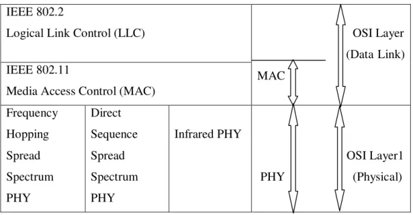
As in all 802.x protocols, 802.11 protocol covers the physical and data link layers. The physical layer is same as in OSI model, but the data link layer is divided into two sub layers one of them is IEEE 802.11 media access control (MAC) and the other is IEEE 802.2 logical link control (LLC) as shown in Figure 2.1. [4]

IEEE 802.2

Logical Link Control (LLC) IEEE 802.11

Media Access Control (MAC)

OSI Layer (Data Link) MAC Frequency Hopping Spread Spectrum PHY Direct Sequence Spread Spectrum PHY Infrared PHY OSI Layer1 PHY (Physical) Table 2.1: IEEE 802.11 standards mapped to the OSI reference model.

The reason why the data link layer is splitted into two sub layers is that MAC layer determines how the channel is allocated and LLC hides the differences between 802.11 variants and make them indistinguishable to higher levels. To manage a shared access medium, the separation of layers is needed in wireless LANs.

(17)

6

2.3 802.11 Physical Layer

As in shown in Figure 2.1, there are three transmission techniques which exists in the physical layer: infrared, frequency hopping spread spectrum (FHSS) and direct sequence spread spectrum (DSSS) [5].

Infrared: This method uses the same technology as in television remote controls. The signals cannot penetrate through the walls so wireless LANs are isolated from each other. Also because of the low data rate (1 Mbps or 2 Mbps), it is not a popular option.

FHSS: The frequency hopping was the first step in the evolution to the DSSS. Here the transmitter sends a frame to receiver within a very short time and afterwards it switches to another frequency by using a pre-defined frequency hopping pattern known by both the transmitter and receiver. FHSS uses 1 MHz bandwidth with 79 channels and the frequency hopping pattern is generated by a pseudorandom number generator. If the stations use the same seed for the pseudorandom number generator and they are synchronized in time, they concurrently hope to the same frequency. This also provides security because the frequency hopping pattern and the amount of time spent in each frequency are known by only transmitter and receiver. The frequency picked up according to the hopping pattern is then modulated using two-level GFSK (Gaussian Frequency Shift Keying) for 1Mbps and four-level GFSK modulation for 2Mbps data rate. The disadvantage of FHSS is that it has low data rate (1 Mbps or 2 Mbps).

DSSS: This is currently one of the most successful data transmission techniques. DSSS is also used in CDMA based cellular networks and Global Positioning Systems (GPS). The idea is to multiply the data being transmitted by a pseudo random binary sequence with a higher bit rate. With DSSS, each bit is transmitted as 11 chips which is called as the Barker sequence and the bit rate of the sequence is called the chipping rate. The data is unrecoverable from the result of such multiplication unless the Barker sequence is known. DSSS also transmits at 1 Mbps or 2 Mbps. In DSSS, phase shift modulation is used. When

(18)

7

operating at 1 Mbps one bit per one Mbaud is transmitted, when operating 2Mpbs two bits per one Mbaud is transmitted.

Because of the limited data rate of FHSS and DSSS, orthogonal frequency division multiplexing (OFDM) technique was introduced for 802.11a and high range direct sequence spread spectrum (HR-DSSS) was introduced for 802.11b. In OFDM, 5 GHz ISM band is used and the speed can reach up to 54 Mbps. There are 52 different frequencies: 48 for data and 4 for synchronization. Since OFDM uses the spectrum efficiently it divides the signal into many narrow bands so transmissions can occur on multiple frequencies at the same time. In HR-DSSS, 11 million chips are used. This is the technique which is used in 802.11b. It works on 2.4 GHz ISM band. 802.11b got popularity very fast because it was in markets before 802.11a. It supports 1, 2, 5.5, and 11Mbps data rates and it is compatible with previous 802.11 standards. The disadvantage of 802.11b is that although there exists 11 channels in 2.4 GHz band only 3 of them are non-overlapping (Channels 1, 6, 11).

802.11g standard which is approved in 2003 uses the OFDM modulation technique. It operates in 2.4 GHz ISM band and up to 54 Mbps data rate is achieved. Since it is compatible with 802.11b and an upgrade is not necessary, it exists as a good choice for users.

A summary of the evolution of wireless network standards is shown in Table 2.2 where high-speed and long-range 802.11 versions, 802.11n and 802.11y, for which standards are currently under development, are also shown.

(19)

8

Evolution of Wireless networking standards

802.11 Protocol Release Frequency (GHz) Data (Mbit/s) Modulation technique Range (Radius Indoor) Depends, # and type of walls Range (Radius Outdoor) Loss includes one wall – 1997 2.4 2 ~20 ~100 a 1999 5 54 OFDM ~35 ~120 b 1999 2.4 11 HR-DSSS ~38 ~140 g 2003 2.4 54 OFDM ~38 ~140 n 2009 2.4, 5 248 OFDM ~70 ~250 y 2008 3.7 54 * ~50 ~5000

Table 2.2: The evolution of 802.11 protocols [6]

* 802.11y uses 802.11a/b/g modulation but on the 3650-3700 MHz band. It is supposed to be exactly the same as 802.11a/b/g, but with a different contention protocol and different MAC layer timing so that it works at much longer ranges.

2.4 802.11 Frequency Spectrum

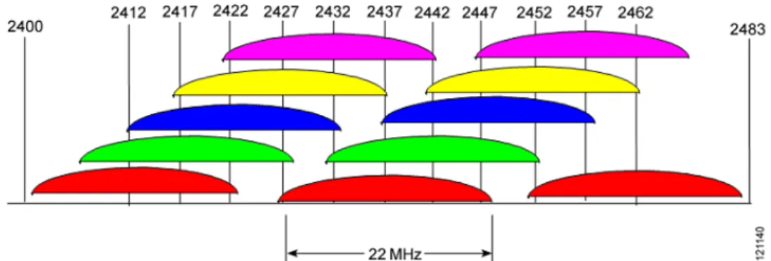
The IEEE 802.11 standard establishes several requirements for the RF transmission characteristics of an 802.11 radio. These are the channelization scheme and how the RF energy spreads across the channel frequencies. The 2.4-GHz band is divided into 11 channels for the FCC or North American domain and 13 channels for the European or ETSI domain. Center frequency separation is only 5 MHz and an overall channel bandwidth is 22 MHz for 802.11b and 802.11g independent of the data rate. Figure 2.2 shows this channelization scheme [7].

(20)

9

Figure 2.1: 802.11 Channelization Scheme

The interference is determined by the level of RF energy that crosses between these channels. The overall energy level drops as the signal spreads farther from the center of the channel. The 802.11b standard defines the required limits for the energy outside the channel boundaries (+/- 11 MHz), also known as the spectral mask. Figure 2.2 shows the 802.11b spectral mask, which defines the maximum permitted energy in the frequencies surrounding the channel’s center frequency [8].

Figure 2.2: 802.11b Spectral Mask

The energy radiated by the transmitter extends well beyond the 22-MHz bandwidth of the channel (+11 MHz from f_c ). At 11 MHz from the center of the channel, the energy must be 30 dB lower than the maximum signal level, and at 22 MHz away, the energy must be 50 dB below the maximum level. As you move farther from the center of the channel, the energy continues to decrease but is still present, providing some interference on several more channels.

(21)

10

2.5 Radio Propagation Models

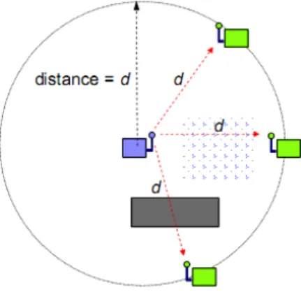
In a mobile system, the characteristics of the used channel are very important. The changes in the channel highly affect the received power. There may be many obstacles in the signal path and typically no line of sight exists between stations. The signal propagates through walls and solid objects and reflections occur often. When using a wireless link, it is essential to study the characteristics related to wave propagation and the environmental factors on the communication link. In order to understand the basics of transmission, the free space propagation is first described below. No disturbances exist in the free space model. It is the basic radio propagation model. Next, two-ray model and shadowing models are discussed [9].

2.5.1 Free Space Propagation

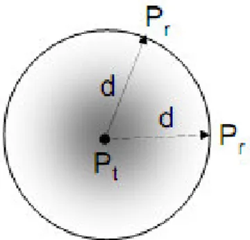
A free space model is the basic model for radio signal propagation. It is assumed that an isotropic antenna is used. An isotropic antenna transmits equally in all directions. The output power is distributed uniformly over the surface of a sphere as shown in Figure 2.3,

Figure 2.3: A typical sphere to find the received power and can be expressed as

2 2 ( / ) 4 t d P S W m d π =

where d is the distance and P_t is the transmitted power. S_d is the distribution of energy distributed over an area. The receiving antenna can be seen as an area

(22)

11

that can absorb the energy in an antenna area A_e. Even if more sophisticated antennas are used, the connection between the antenna gain G and the area A_e is described by 2 2 2 2 ( ) 4 4 e G Gc A m f λ π π = =

Here c is the speed of an electromagnetic wave, approximately equal to the speed of light. If the above two equations are combined, the connection between the received signal power P_r and the other parameters such as transmitted power Pt, antenna gain G and signal frequency can be expressed as

2 2 P . (4 ) t r r e PGc S A fd π = =

There is direct connection between the received signal power and the chosen carrier frequency. The detected signal power is reciprocally proportional to the square of the frequency and square of the distance between the antennas. In order to increase the received signal power, one solution is to use a higher transmission power; another is to lower the carrier frequency or use antennas with a larger gain. In the free space model, no interference occurs and no obstacles are present.

2.5.2 Two-ray Model

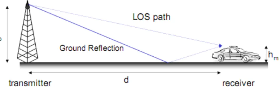
In reality, we do not have a single signal arriving to a receiver. We may have multiple signals arriving to a receiver from the same source. In Figure 2.4, we see two rays arriving to a receiver.

(23)

12

Figure 2.4: Two-ray model

In the two-ray model, where there are both a direct path and ground reflected propagation path between the transmitter and receiver antennas, the relationship between received power and transmit power is approximated by:

2 2 4 t r r t t r h h P PG G d = t P: Transmit power (W or mW) r P : Received power (W or mW) t

G : The transmit antenna gain

r

G : The receive antenna gain

t

h : Height of transmitter antenna (m)

r

h : Height of receiver antenna (m)

(24)

13

2.5.3 Effect of shadowing

Although the distance is the same, there may be different objects in between. This causes the received power to be different depending on the location (although the distance between transmitter and receiver remains the same). This can be observed in Figure 2.5.

Figure 2.5: Effect of shadowing.

The free space model and the two-ray model predict the received power as a deterministic function of distance. They both represent the communication range as an ideal circle. In reality, because of the multi path propagation effects the received power at certain distance is a random variable which is the case for shadowing model. In fact, the above two models predict the mean received power at distance. Shadowing model is more general and widely-used than free-space and two-ray models [10].

The shadowing model has two parts. The first one is known as the path loss model. This part predicts the mean received power at distance d which is denoted by P ( )d

r . It uses (d0) as a reference point. The received power at a distance d relative to d0 can be computed as:

0 r r 0 P ( ) P ( ) d d d d β     =    _ _   _ _

(25)

14

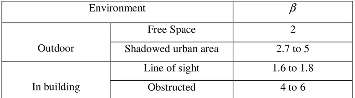
Here β is called the path loss exponent, which indicates the rate at which the path loss increases with distance. The value of path loss exponent depends on the specific propagation environment and is usually determined by field measurement. So larger values correspond to more obstructions and hence faster decrease in average received power as distance becomes larger. P ( )

0

d

r can be

calculated from the free space model. Table 2.3 provides path loss exponents for different propagation environments. So path loss from the above equation can be found as (in dB) : r 0 0 r P ( ) 10 log( / ) P ( ) db d d d d β   = −      

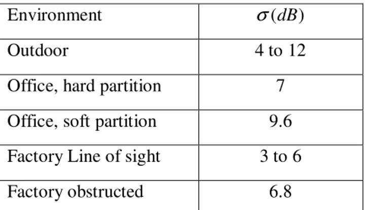
The second part of the shadowing model is a log-normal random variable, that is, Gaussian distributed measured in dB. This part deals with the variation of the received power at a certain distance. The overall shadowing model is represented by r r 0 0 P ( ) 10 log( / ) P ( ) db db d d d X d

β

  = − +    

Here Xdb is a Gaussian random variable with zero mean and standard deviation

(σ ). The shadowing model extends the ideal circle model to a richer statistical model: nodes can only probabilistically communicate when they are close to the edge of the communication range [10].

Environment β

Free Space 2

Outdoor Shadowed urban area 2.7 to 5

Line of sight 1.6 to 1.8

In building Obstructed 4 to 6

Table 2.3: Path Loss Exponents for Different Environments

(26)

15

Environment σ(dB)

Outdoor 4 to 12

Office, hard partition 7

Office, soft partition 9.6

Factory Line of sight 3 to 6

Factory obstructed 6.8

Table 2.4: Some typical value of shadowing deviation in dB

2.6 Access Point Selection Problem

WLANs have become are quite popular in the last decade. As the costs of wireless Access Points (APs) and wireless Network Interface Card (NIC) have been decreasing, WLANs became the preferred technology of access in homes, offices, shopping centers etc. A wireless AP is a base station in wireless networks which is typically a wireless Ethernet (Wi-Fi) LAN. They are stand- alone devices that plug into an Ethernet switch or hub. An AP connects users to other users within the network and also can serve as the point of interconnection between the WLAN and a fixed wired network. Each AP can serve multiple users within its range. As people move beyond the range of one AP, they are automatically handed over to the next one. A small WLAN may only require a single access point, but as number of users in the network and the physical size of the network increase, more APs are necessary to cover a certain service area. On the other hand, if we increase the number of APs, a station can potentially associate with more than one APs. Here the AP selection problem arises, which AP will be selected by that station among the candidate APs. In 802.11, a station is associated to an AP with the strongest received signal strength. However, this may result in significant load imbalance between the APs. Some of APs may serve too many stations but some of them may be lightly loaded or even idle because of inappropriate AP selection. This causes degradation in overall network throughput.

(27)

16

If you are a home user or working in a small office, one AP is already enough and there does not exist many problems except some interference from cordless phones and microwave ovens. However, in a large company which has many floors you may need more than one AP, may be 10, 20 or even more which depends on the power supply needs, the thickness of walls and infrastructure of the building. Many parameters should be taken into account in order to make a correct decision about where to place APs and how many APs are necessary, etc.

Each AP covers a certain area according to it’s transmit power. While placing the APs, we should be very careful such that there should not be coverage gaps in the service area. When we increase the transmit power of APs, many stations may associate with that AP and that seems as if a good solution to eliminate the coverage overlaps among AP’s. However, in this case interference problem arises among the APs in the coverage area as well external interference created by microwaves, 2.4GHz phones, Bluetooth-enabled devices, or other RF sources. This can significantly degrade the performance of our wireless LAN. Radio frequency (RF) interference can lead to many problems on wireless LAN deployments.

Optimal access point selection is a crucial problem in the deployment of IEEE 802.11 WLAN networks. APs should provide adequate bandwidth to users around them. APs should cover all users in a demand cluster (DC) but it is not always the case because the received signal weakens as it propagates; as a result of this if the received signal is not above a threshold level, the user cannot reach the corresponding AP. Also if the received signal does not provide a minimum SINR condition, very low data rates can be seen which results in poor network utilization. We can cover a certain area by a large number of APs but they are expensive equipments. Our aim is to provide enough signal level and bandwidth to the users by using a small number of APs. With our Optimal Access Point Selection Algorithm, which we will focus in the next chapter, we balance the traffic loads in APs and a DC should not need to connect to the closest AP but it is connected to the one which may be farther away but less congested. By

(28)

17

minimizing the traffic loads in heavily congested APs, we try to balance the loads at APs which results with a higher throughput in wireless network.

2.6.1 Previous Work on AP Selection

In [11], the authors formulate different optimization problems with various objective functions. The considered variables are positions of APs, their heights, their transmission power levels, and antenna sectorization. This paper offers different precise objective functions for the positioning problem, and the corresponding mathematical methods to achieve optimal solutions. The optimization problems maximize the number of covered demand nodes while penalizing multiple coverage of demand nodes.

In [12], the authors use a algorithm to solve the AP selection problem. The algorithm begins with a set of potential locations for APs. In each step, a new AP is picked from the set that covers the maximum number of uncovered demand nodes. This algorithm assumes that if an AP covers the most demand nodes, it is more desirable to select it.

In [13], the authors formulate an integer linear programming problem for optimizing AP selection. The algorithm maximizes the throughput by considering load balancing among APs. The optimization objective is to minimize the maximum congested APs.

In [14], the authors use a divide-and-conquer algorithm to select APs. The total service area is divided into equally sized squares with the algorithm. The problem is then solved in each of these divisions by exhaustive search.

In [15], this work presents a very simple and efficient integrated integer linear programming optimization model for solving both base station selection and fixed frequency channel assignment problems in indoor environments. The algorithm minimizes the number of APs that cover a desired service area.

In [16], the author points out necessary precautions while designing a large scale wireless network. This work says how to place APs to minimize the gaps

(29)

18

between the APs. Also says while serving in high density areas increasing the receiver threshold for to reduce APs’ coverage area is useful.

In [17], the authors design a WLAN especially one with a large number of APs by using a design tool called Rollabout. Properly solving the selection of access point locations and access point frequency assignments issues involves a trial and error process, and can be very time consuming. The Rollabout design tool partially automates this process, making it quicker and more efficient. With Rollabout, data collection is much faster, and a much larger set of data can be captured. Furthermore, the design tool predicts the coverage changes that will result when access points are moved to different locations. It can also produce an optimal set of frequency assignments for any set of access point locations and corresponding coverage areas. With this tool you can make a good WLAN design and also speed the design process.

There are studies regarding the optimal AP selection in IEEE 802.11 networks but they only take into consideration only one of the minimum signal level (S

thres) or minimum Signal to Noise and Interference (SINRmin) constraints.

In this thesis we use both constraints. WLAN designs using both orthogonal (Using Channels 1, 6, 11) and non-orthogonal (Using partially overlapping channels 1, 4, 7, 11) channels are realized for two different buildings. Only orthogonal (non-overlapping) channels have been used in previous work whereas non-orthogonal overlapping channels are also considered in this thesis.

(30)

19

Chapter 3 Optimal Access Point Selection

Algorithm

In this chapter, we introduce the proposed Optimal Access Point Selection formulation and its solution. First, the constraints in AP selection are discussed. Next, the Mixed Integer Linear Programming formulation is explained and lastly numerical results are shown. We test our formulation in two different building structures. One of them is a three story and the other is a U-shaped building. We run the algorithm both in orthogonal (by using 3 non-overlapping channels 1, 6, 11) and non-orthogonal channels (by using 4 overlapping channels 1, 4, 7, 11) and compare the results.

3.1 Constraints in AP Selection Algorithm

In our algorithm, there are four constraints: 1. Minimum signal level (S

thres) constraint

2. Minimum Signal-to-Noise and Interference (SINR) ratio constraint 3. AP transmit power constraint

4. Number of connected APs constraint

Let us explain these constraints qualitatively and quantitatively. 1. Minimum signal level (S

thres) constraint: This constraint, which is also called Receiver sensitivity is a very important figure for wireless LAN equipment. This is the minimum required signal level for a DC to associate with an AP. If the measured signal level from an AP in a DC is above the S

thres level, this means that DC may connect to that AP and conversely if the measured signal level from an AP at a DC is below the S

(31)

20

connect to that AP. Of course, a DC may get multiple signals that are above the S

thres multiple APs around it. This time our Optimal Access Point Selection Algorithm takes turn and chooses the AP which is less congested compared to other APs. Receiver sensitivity for an 802.11 transceiver ranges between -85dB and -78dB for different brands. The best preferred receiver sensitivity is the smallest, i.e. -85dB is better than -78dB. This corresponds to a difference of 7dB in available signal, which corresponds to a range improvement of over 2x with the free space propagation model. If the received signal level at DC i received from AP j is shown by S

ij and Xij being the decision variable describing whether DC i is connected to AP j,

1

X

ij = only if Sij>Sthres (3.1) In our tests we set S

thres to -80 dBm.

2. Minimum Signal-to-Noise+Interference (

min

SINR ) ratio: Signal-to-Noise+Interference (SINR) ratio is the received signal level (in dBm) minus the noise+interference level (in dBm). It measures the clarity of the signal in a wireless transmission channel. Usually if the signal power is less than or just equals the noise power it is not detectable. For a signal to be detected, the signal energy plus the noise energy must exceed some threshold value. SINR is a required minimum ratio, if N is increased, then S must also be increased to maintain that threshold. SINR directly impacts the performance of a wireless LAN connection. A higher SINR value means that the signal strength is stronger in relation to the noise+interference levels, which allows higher data rates and fewer retransmissions all of which offers better throughput. Of course the opposite is also true. A lower SINR requires wireless LAN devices to operate at lower data rates, which decreases throughput. Again if the received signal level at DC i of the AP j is shown by S

(32)

21 1 X ij = only if min (3.2) S ij SINR Noise S W ik kj k j > + ∑ × ≠

Here noise is assumed to be White Gaussian Noise and W

kj is the overlapping channel interference factor. In the non-orthogonal condition, we use partially overlapping channels (1, 4, 7, 11) We model inter-channel interference (ICI) by defining an overlapping channel interference factor, W

ij, to be the relative percentage increase in interference as a result of two APs i and j using overlapping channels. The used frequencies of the channels are as we studied in Section 2.4. S W

ik× kj means the interference at the DC i which is a result of inter channel interference (ICI) from partially overlapping channels from the other APs around the AP j. In our tests, we set

min

SINR to 6 dB.

The inter-channel interference factor is calculated as fallows: In the non-orthogonal channels case, we use partially overlapping 1, 4, 7, 11 channels.

To calculate inter-channel interference factor W

ij we use the attenuation values in Table 3.1 which is the result of an experimental study in [18]. For example, if a receiver is tuned to channel 1, it will receive all transmissions on channel 1 without attenuation, but interfering transmissions produced in channel 4, are reduced by more than 8dB.

i− j 0 1 2 3 4 5

W

ij , dB 0 - 0.28 - 2.19 - 8.24 - 25.50 - 49.87

Table 3.1: Inter-channel interference factor

3. AP transmit power constraint: In most cases, the transmit power should be set to the highest value. This maximizes the range, which reduces the number of wireless access points and cost of the system in the service area. On the hand, if we increase transmit power too much, this makes AP more sensitive to interference. Lower power settings also limit the wireless signals from

(33)

22

propagating outside the physically controlled area of the facility, which improves security. In our tests, we set the transmit power of APs to 30 mW. 4. Number of connected APs constraint: A DC may get more than one signal which is above the S

thres from the APs around it. To balance the traffic load on each AP we want each DC to connect only one AP at a time, so we reach a higher network throughput which yields better utilization.

3.2 MILP Formulation of AP Selection Problem

Our stepwise approach to the AP selection problem is as follows:

First, we create a service area map. We divide a service area into smaller demand clusters. In each demand cluster, the number of users and traffic requirement are known. An example of service area map for a three story building with 70 demand clusters is shown in Figure 3.1.

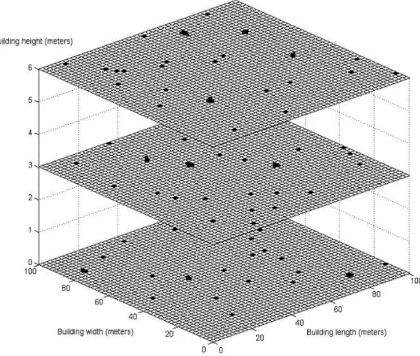
Next, we create signal level map. By using a propagation model, signal levels in each demand cluster is measured or estimated. Of course, the signal level in DCs must be above a threshold value in order to provide sufficient signal to noise ratio. As an example of signal level map for a three story building with 14 APs is shown in Figure 3.2.

Then, we place the candidate APs by considering the wired LANs power supply and installation costs.

Next, we select the APs from among a set of candidate locations. For this, we use the service area and signal level map. We increase the network throughput by minimizing the number of bottleneck APs by balancing the traffic load. Finally, we assign frequencies to APs for minimizing the interference.

(34)

23

Figure 3.1: A service area map for a three story building with 70 demand clusters

(35)

24

Figure 3.2: A signal level map for a three story building with 14 APs [19]

The list of parameters and variables used in the AP selection formulation is given below:

i : index for DCs j : index for APs

L: The total number of demand clusters. N: The total number of candidate APs S

ij: The received signal level at DC iof AP j D

i: Demand cluster i

d

ij: Distance between DC iand AP j

P

i: Transmit power of AP i B

(36)

25 X

ij: Decision variable which is 1 if DC iis assigned to AP j, 0 otherwise T

i: Average traffic load of DC i W

ij: Overlapping channel interference factor M : A fixed integer number

S

thres: Minimum acceptable signal level for a DC to connect an AP

min

SINR : Minimum ratio of the received signal level and the noise+interference level so that a DC can be connected to an AP.

MaxCon: Maximum Congestion

(

)

min MaxCon 3.3 Subject to

(

)

1... 3.4 X i L ij j N = ∀ ∈ ∑ = 1 (3.5) 1 L C T X j _B i ij i j = ∑ × = (3.6) MaxCon C j j ≥ ∀ ( ) 1 (3.7) S S ij thres X ij _M − ≤ +

(

)

min min 1 3.8

S SINR S W Noise SINR

ij ik kj k j X ij _M − × ∑ × − × ≠ ≤ +         Our goal is to minimize the maximum congested access point. By this way we balance the traffic load in each access point which improves the overall throughput in the network.

(37)

26

Constraint (3.5) defines the congestion factor of an AP.

Constraint (3.6) states that the defined variable MaxCon should be greater than the congestion factor of an AP.

Constraint (3.7) states that decision variable X_ij maybe one only if the signal level in that DC is above a threshold level (S

thres). This constraint is the linearized form of the equation (3.1) so that the AP selection problem can be formulated as a MILP. In this constraint, M is large integer known as “big M” taken as 100 in our numerical studies.

Constraint (3.8) states that X

ij can be one only if the measured signal level provides the

min

SINR constraint. This constraint depends on the interference which is the result of partially overlapped APs and noise in that channel. This constraint is the linearized form of the equation (3.2). Again, M corresponds to “big M” (M=100 is used).

3.3 Numerical Results

We used General Algebraic Modeling System (GAMS) to solve this mixed integer optimization problem. We tested our algorithm in two different building structures. One of them is U-shaped (100mx100mx100m) and the other one is a three story 100mx100m building. We have 21 APs and 30 DCs in the U-shaped building and 14 APs and 20 DCs in the three story building. The number of users per demand cluster is uniformly distributed between 1 and 10 in each DC. The average traffic demand per user is assumed to be 200 Kbps, and each AP has a maximum bandwidth of 11 Mbps. The average traffic load of a demand cluster T

i, can be calculated as the number of users in demand cluster i multiplied by the average traffic demand per user.

(38)

27

3.3.1 Numerical Results for Orthogonal Channel Assignment

We first test the proposed AP selection formulation on a three-story building using non-overlapping channels 1, 6, 11 only).

The average traffic load at each DC used in the analysis is given in Table 3.2

T1 1600 T11 1400 T2 2000 T12 2000 T3 800 T13 1800 T4 1800 T14 400 T5 1200 T15 400 T6 400 T16 2000 T7 800 T17 200 T8 400 T18 800 T9 1800 T19 800 T10 1600 T20 400

Table 3.2: The average traffic load for each DC (Kbps).

We generated a candidate AP assignment graph from our service area map and signal level map. From the candidate AP assignment graph, we observe that all the DCs are connected to at least one AP, but some DCs are connected to more than one AP.

(39)

28

ij

X AP1 AP2 AP3 AP4 AP5 AP6 AP7 AP8 AP9 AP10 AP11 AP12 AP13 AP14

DC1 0 0 0 0 0 1 0 0 0 0 0 0 0 0 DC2 0 1 1 0 0 0 0 0 0 0 0 0 0 0 DC3 0 1 1 0 0 0 0 0 0 0 0 0 0 0 DC4 0 0 0 1 0 0 0 0 0 0 0 0 0 0 DC5 0 0 0 0 0 0 0 1 0 0 0 0 0 0 DC6 0 0 0 0 0 1 0 0 0 0 0 0 0 0 DC7 0 1 1 0 0 0 0 1 0 0 0 0 0 0 DC8 0 0 1 0 0 0 0 0 0 1 0 0 0 0 DC9 1 1 0 0 0 0 0 0 0 1 0 0 0 0 DC10 0 0 0 0 1 1 0 0 0 0 0 0 1 1 DC11 0 0 0 1 0 0 1 0 0 0 0 1 0 0 DC12 0 0 0 0 0 1 0 1 0 0 0 0 0 1 DC13 0 0 0 1 1 0 0 0 0 1 0 1 0 0 DC14 0 0 0 0 0 0 1 1 0 1 0 1 0 0 DC15 0 0 0 0 0 0 0 0 0 1 1 0 0 0 DC16 0 0 0 0 0 0 0 0 0 0 0 0 1 1 DC17 0 0 0 0 0 0 0 0 1 1 0 0 0 0 DC18 0 0 0 0 0 0 0 1 0 0 1 0 0 0 DC19 0 0 0 0 0 0 1 0 0 0 0 1 1 0 DC20 0 0 0 0 0 0 1 0 0 0 0 1 0 0

Table 3.3: Candidate AP assignment graph for 3 story building.

We see from Table 3.3 that a DC i, may be connected to multiple APs if the signal level, S

ij, of an AP j at Di is greater than Sthres . For instance, DC2 is connected to AP 2 and AP 3 while DC1 is connected to AP 6 only. Also, demand clusters, DC8 through DC13 located on the second floor, are connected to more APs than demand clusters located on other floors since ample signals can be received from both the first and third floors.

Table 3.4 is the result of the AP selection formulation obtained by using GAMS in case of orthogonal channels.

(40)

29

ij

Table 3.4: The results of optimization in case of orthogonal condition (1, 6, 11) for 3 story building.

(41)

30

The assignments of DCs to APs are shown in Figure 3.3

Figure 3.3: The assignment figure of APs and DCs in the orthogonal condition Then, we tested the formulation on U-shaped building which is shown

in Figure 3.4 using orthogonal channels.

(42)

31 T1 1600 T11 1400 T21 800 T2 2000 T12 2000 T22 400 T3 800 T13 1800 T23 1200 T4 1800 T14 400 T24 1600 T5 1200 T15 400 T25 200 T6 400 T16 2000 T26 1800 T7 800 T17 200 T27 800 T8 400 T18 800 T28 2000 T9 1800 T19 800 T29 400 T10 1600 T20 400 T30 1200

Table 3.5: The average traffic load for each DCs for U-shaped building Candidate AP assignment graph for the U-shaped building is given in Table 3.7. In this building, we have 21 APs and 30 DCs. We observe from Table 3.7 that a demand cluster i, may be connected to multiple APs if the signal level, S

ij, of an AP j at D

i is greater than a given threshold. For instance, D2 is connected to AP1, AP2 and AP3 and D30 is connected to AP20 and AP21. Also, demand clusters, DC6, DC7, DC13 and DC14 are connected to more APs than other demand clusters because these are located in the mid points of the building. Table 3.8 is the result of the AP selection formulation for orthogonal channels.

(43)

32

(44)

33 ij X AP 1 AP 2 AP 3 AP 4 AP 5 AP 6 AP 7 AP 8 AP 9

AP10 AP11 AP12 AP13 AP14 AP15 AP16 AP17 AP18 AP19 AP20 AP21 DC1 1 1 0 0 0 0 0 0 0 0 0 0 0 0 0 0 0 0 0 0 0 DC2 1 1 1 0 0 0 0 0 0 0 0 0 0 0 0 0 0 0 0 0 0 DC3 0 1 1 0 0 0 0 0 0 0 0 0 0 0 0 0 0 0 0 0 0 DC4 0 0 1 1 1 0 0 0 0 0 0 0 0 0 0 0 0 0 0 0 0 DC5 0 0 0 1 1 0 0 0 0 0 0 0 0 0 0 0 0 0 0 0 0 DC6 0 0 0 0 1 1 1 1 0 0 0 0 0 0 0 0 0 0 0 0 0 DC7 0 0 0 0 0 1 1 1 0 0 0 0 0 0 0 0 0 0 0 0 0 DC8 0 0 0 0 0 1 1 1 1 0 0 0 0 0 0 0 0 0 0 0 0 DC9 0 0 0 0 0 1 1 1 0 0 0 0 0 0 0 0 0 0 0 0 0 DC10 0 0 0 0 0 1 1 1 1 0 0 0 0 0 0 0 0 0 0 0 0 DC11 0 0 0 0 0 0 1 1 1 0 0 0 0 0 0 0 0 0 0 0 0 DC12 0 0 0 0 0 0 0 1 1 0 0 0 0 0 0 0 0 0 0 0 0 DC13 0 0 0 0 0 0 0 0 1 1 1 0 0 0 0 0 0 0 0 0 0 DC14 0 0 0 0 0 0 0 0 0 1 1 0 0 0 0 0 0 0 0 0 0 DC15 0 0 0 0 0 0 0 0 0 0 1 1 0 0 0 0 0 0 0 0 0 DC16 0 0 0 0 0 0 0 0 0 0 1 1 0 0 0 0 0 0 0 0 0 DC17 0 0 0 0 0 0 0 0 0 0 0 1 1 0 0 0 0 0 0 0 0 DC18 0 0 0 0 0 0 0 0 0 0 0 1 1 1 0 0 0 0 0 0 0 DC19 0 0 0 0 0 0 0 0 0 0 0 1 1 1 0 0 0 0 0 0 0 DC20 0 0 0 0 0 0 0 0 0 0 0 0 1 1 1 1 0 0 0 0 0 DC21 0 0 0 0 0 0 0 0 0 0 0 0 0 1 1 1 0 0 0 0 0 DC22 0 0 0 0 0 0 0 0 0 0 0 0 0 0 1 1 1 0 0 0 0 DC23 0 0 0 0 0 0 0 0 0 0 0 0 0 0 1 1 0 0 0 0 0 DC24 0 0 0 0 0 0 0 0 0 0 0 0 0 0 0 1 1 0 0 0 0 DC25 0 0 0 0 0 0 0 0 0 0 0 0 0 0 0 0 1 1 0 0 0 DC26 0 0 0 0 0 0 0 0 0 0 0 0 0 0 0 0 1 1 0 0 0 DC27 0 0 0 0 0 0 0 0 0 0 0 0 0 0 0 0 0 1 1 0 0 DC28 0 0 0 0 0 0 0 0 0 0 0 0 0 0 0 0 0 1 1 0 0 DC29 0 0 0 0 0 0 0 0 0 0 0 0 0 0 0 0 0 0 1 1 0 DC30 0 0 0 0 0 0 0 0 0 0 0 0 0 0 0 0 0 0 0 1 1

(45)

34 ij X AP 1 AP 2 AP 3 AP 4 AP 5 AP 6 AP 7 AP 8 AP 9

AP10 AP11 AP12 AP13 AP14 AP15 AP16 AP17 AP18 AP19 AP20 AP21

DC1 0 1 0 0 0 0 0 0 0 0 0 0 0 0 0 0 0 0 0 0 0 DC2 1 0 0 0 0 0 0 0 0 0 0 0 0 0 0 0 0 0 0 0 0 DC3 0 0 1 0 0 0 0 0 0 0 0 0 0 0 0 0 0 0 0 0 0 DC4 0 0 0 1 0 0 0 0 0 0 0 0 0 0 0 0 0 0 0 0 0 DC5 0 0 0 0 1 0 0 0 0 0 0 0 0 0 0 0 0 0 0 0 0 DC6 0 0 0 0 1 0 0 0 0 0 0 0 0 0 0 0 0 0 0 0 0 DC7 0 0 0 0 0 0 0 1 0 0 0 0 0 0 0 0 0 0 0 0 0 DC8 0 0 0 0 0 1 0 0 1 0 0 0 0 0 0 0 0 0 0 0 0 DC9 0 0 0 0 0 0 1 0 0 0 0 0 0 0 0 0 0 0 0 0 0 DC10 0 0 0 0 0 1 0 0 0 0 0 0 0 0 0 0 0 0 0 0 0 DC11 0 0 0 0 0 0 0 1 0 0 0 0 0 0 0 0 0 0 0 0 0 DC12 0 0 0 0 0 0 0 0 1 0 0 0 0 0 0 0 0 0 0 0 0 DC13 0 0 0 0 0 0 0 0 0 0 1 0 0 0 0 0 0 0 0 0 0 DC14 0 0 0 0 0 0 0 0 0 1 0 0 0 0 0 0 0 0 0 0 0 DC15 0 0 0 0 0 0 0 0 0 0 1 0 0 0 0 0 0 0 0 0 0 DC16 0 0 0 0 0 0 0 0 0 0 0 1 0 0 0 0 0 0 0 0 0 DC17 0 0 0 0 0 0 0 0 0 0 0 0 1 0 0 0 0 0 0 0 0 DC18 0 0 0 0 0 0 0 0 0 0 0 0 0 1 0 0 0 0 0 0 0 DC19 0 0 0 0 0 0 0 0 0 0 0 0 1 0 0 0 0 0 0 0 0 DC20 0 0 0 0 0 0 0 0 0 0 0 0 1 0 0 0 0 0 0 0 0 DC21 0 0 0 0 0 0 0 0 0 0 0 0 0 1 0 0 0 0 0 0 0 DC22 0 0 0 0 0 0 0 0 0 0 0 0 0 0 1 0 0 0 0 0 0 DC23 0 0 0 0 0 0 0 0 0 0 0 0 0 0 1 0 0 0 0 0 0 DC24 0 0 0 0 0 0 0 0 0 0 0 0 0 0 0 1 0 0 0 0 0 DC25 0 0 0 0 0 0 0 0 0 0 0 0 0 0 0 0 1 0 0 0 0 DC26 0 0 0 0 0 0 0 0 0 0 0 0 0 0 0 0 1 0 0 0 0 DC27 0 0 0 0 0 0 0 0 0 0 0 0 0 0 0 0 0 0 1 0 0 DC28 0 0 0 0 0 0 0 0 0 0 0 0 0 0 0 0 0 0 1 0 0 DC29 0 0 0 0 0 0 0 0 0 0 0 0 0 0 0 0 0 0 0 1 0 DC30 0 0 0 0 0 0 0 0 0 0 0 0 0 0 0 0 0 0 0 0 1

(46)

35

3.3.2 Numerical Results for Non-Orthogonal Channel Assignment

Table 3.8 is the result of the AP selection formulation obtained using

non-orthogonal channels (partially overlapped channels 1, 4, 7, 11) for three story building. The same candidate assignment graph is used as in the orthogonal condition. The assignments between the APs and DCs are shown in Figure 3.5.

ij

Table 3.8: The result of optimization in case of non-orthogonal condition for 3 story building (1,4,7,11)

(47)

36

Figure 3.5: The matching figure of the APs and DCs in non-orthogonal condition

(48)

37

Table 3.9 is the result of the AP selection formulation using non-orthogonal channels for the U-shaped building. The same candidate assignment graph is used as in the orthogonal channel assignment. It is observed that the congestion of APs is distributed throughout the network to avoid bottleneck APs.

(49)

38 ij

X AP AP AP AP AP AP AP AP AP AP10 AP11 AP12 AP13 AP14 AP15 AP16 AP17 AP18 AP19 AP20 AP21

DC1 0 1 0 0 0 0 0 0 0 0 0 0 0 0 0 0 0 0 0 0 0 DC2 1 0 0 0 0 0 0 0 0 0 0 0 0 0 0 0 0 0 0 0 0 DC3 0 0 1 0 0 0 0 0 0 0 0 0 0 0 0 0 0 0 0 0 0 DC4 0 0 0 1 0 0 0 0 0 0 0 0 0 0 0 0 0 0 0 0 0 DC5 0 0 0 0 1 0 0 0 0 0 0 0 0 0 0 0 0 0 0 0 0 DC6 0 0 0 0 1 0 0 0 0 0 0 0 0 0 0 0 0 0 0 0 0 DC7 0 0 0 0 0 0 0 1 0 0 0 0 0 0 0 0 0 0 0 0 0 DC8 0 0 0 0 0 1 0 0 1 0 0 0 0 0 0 0 0 0 0 0 0 DC9 0 0 0 0 0 0 1 0 0 0 0 0 0 0 0 0 0 0 0 0 0 DC10 0 0 0 0 0 1 0 0 0 0 0 0 0 0 0 0 0 0 0 0 0 DC11 0 0 0 0 0 0 0 1 0 0 0 0 0 0 0 0 0 0 0 0 0 DC12 0 0 0 0 0 0 0 0 1 0 0 0 0 0 0 0 0 0 0 0 0 DC13 0 0 0 0 0 0 0 0 0 0 1 0 0 0 0 0 0 0 0 0 0 DC14 0 0 0 0 0 0 0 0 0 1 0 0 0 0 0 0 0 0 0 0 0 DC15 0 0 0 0 0 0 0 0 0 0 1 0 0 0 0 0 0 0 0 0 0 DC16 0 0 0 0 0 0 0 0 0 0 0 1 0 0 0 0 0 0 0 0 0 DC17 0 0 0 0 0 0 0 0 0 0 0 0 1 0 0 0 0 0 0 0 0 DC18 0 0 0 0 0 0 0 0 0 0 0 0 0 1 0 0 0 0 0 0 0 DC19 0 0 0 0 0 0 0 0 0 0 0 0 1 0 0 0 0 0 0 0 0 DC20 0 0 0 0 0 0 0 0 0 0 0 0 1 0 0 0 0 0 0 0 0 DC21 0 0 0 0 0 0 0 0 0 0 0 0 0 1 0 0 0 0 0 0 0 DC22 0 0 0 0 0 0 0 0 0 0 0 0 0 0 1 0 0 0 0 0 0 DC23 0 0 0 0 0 0 0 0 0 0 0 0 0 0 1 0 0 0 0 0 0 DC24 0 0 0 0 0 0 0 0 0 0 0 0 0 0 0 1 0 0 0 0 0 DC25 0 0 0 0 0 0 0 0 0 0 0 0 0 0 0 0 1 0 0 0 0 DC26 0 0 0 0 0 0 0 0 0 0 0 0 0 0 0 0 1 0 0 0 0 DC27 0 0 0 0 0 0 0 0 0 0 0 0 0 0 0 0 0 0 1 0 0 DC28 0 0 0 0 0 0 0 0 0 0 0 0 0 0 0 0 0 1 0 0 0 DC29 0 0 0 0 0 0 0 0 0 0 0 0 0 0 0 0 0 0 1 0 0 DC30 0 0 0 0 0 0 0 0 0 0 0 0 0 0 0 0 0 0 0 1 0

(50)

39

3.3.3 Comparisons and detailed analysis

In this section we discuss the results of the formulation and effects of the parameters on the results.

3.3.3.1 Effect of Orthogonality

We observe from Table 3.4 and Table 3.8 that some of the DCs are connected to different APs. These are summarized in the Table 3.10. This may be expected because when orthogonal and non-orthogonal channels are used in the non-orthogonal case, the

min

SINR constraint has much more dominant effect than the orthogonal channel assignment.

DCs Orthogonal Condition Non-orthogonal Condition

DC10 AP5 AP4

DC13 AP5 AP4

DC17 AP10 AP9

Table 3.10: Matching differences in orthogonal and non-orthogonal condition

3.3.3.2. Effect of Average Traffic Rate

Here, we discuss how the DC-AP assignments change on the average traffic rate increases. The resulting assignments are shown in Table 3.11 and Table 3.12, respectively.

The differences are shown in red. As we see in the case of orthogonal condition when the average traffic rate is 4x and in the case of non-orthogonal condition when the average traffic rate is 3x some of the DCs are connected to different APs. The reason of this is the increased congestion at some APs. Furthermore, if we increase the average traffic rate more, we observe that numbers of DCs which are connected to different APs are increase. The results obtained here are valid both in orthogonal and non-orthogonal conditions.

(51)

40

Connected AP’s in case of different traffic rates

DCs Av.trf.rate 1 X 2 X 3 X 4 X

1 1600 AP6 AP6 AP6 AP6

2 2000 AP3 AP3 AP3 AP3

3 800 AP2 AP2 AP2 AP2

4 1800 AP7 AP7 AP7 AP4

5 1200 AP8 AP8 AP8 AP8

6 400 AP6 AP6 AP6 AP6

7 800 AP2 AP2 AP2 AP2

8 400 AP11 AP11 AP11 AP11

9 1800 AP1 AP1 AP1 AP1

10 1600 AP5 AP5 AP5 AP5

11 1400 AP12 AP12 AP12 AP7

12 2000 AP14 AP14 AP14 AP14

13 1800 AP4 AP4 AP4 AP12

14 400 AP10 AP10 AP10 AP10

15 400 AP10 AP10 AP10 AP10

16 2000 AP13 AP13 AP13 AP13

17 200 AP9 AP9 AP9 AP9

18 800 AP11 AP11 AP11 AP11

19 800 AP12 AP12 AP12 AP7

20 400 AP7 AP7 AP7 AP12

Table 3.11: Connected AP’s in case of different traffic rates in case of orthogonal condition

Optimal access point selection in multi-channel IEEE 80211 networks

OPTIMAL ACCESS POINT SELECTION IN

MULTI-CHANNEL IEEE 802.11 NETWORKS

By

Mustafa AYDINLI

September 2008

ABSTRACT

OPTIMAL ACCESS POINT SELECTION IN

MULTI-CHANNEL IEEE 802.11 NETWORKS

ÖZET

ÇOK KANALLI KABLOSUZ 802.11 AĞLARDA

ERİŞİM CİHAZLARININ OPTİMİZASYONU

ACKNOWLEDGEMENTS

Table of Contents

List of Figures

List of Tables

Acronyms

Chapter 1

Introduction

Chapter 2

IEEE 802.11 protocol and

Specifications

2.1 IEEE 802.11 general principles

2.2 802.11 Protocol Stack

2.3 802.11 Physical Layer

2.4 802.11 Frequency Spectrum

2.5 Radio Propagation Models

β

2.6 Access Point Selection Problem

Chapter 3

Optimal Access Point Selection

Algorithm

3.1 Constraints in AP Selection Algorithm

3.2 MILP Formulation of AP Selection Problem

(

)

(

)

(

)

3.3 Numerical Results