Optimal investment under transaction costs: A threshold rebalanced portfolio approach

Optimal Investment Under Transaction Costs: A

Threshold Rebalanced Portfolio Approach

Sait Tunc, Mehmet Ali Donmez, and Suleyman Serdar Kozat, Senior Member, IEEE

Abstract—We study how to invest optimally in a financial

market having a finite number of assets from a signal processing perspective. Specifically, we investigate how an investor should distribute capital over these assets and when he/she should real-locate the distribution of the funds over these assets to maximize the expected cumulative wealth over any investment period. In particular, we introduce a portfolio selection algorithm that maximizes the expected cumulative wealth in i.i.d. two-asset discrete-time markets where the market levies proportional trans-action costs in buying and selling stocks. We achieve this using “threshold rebalanced portfolios”, where trading occurs only if the portfolio breaches certain thresholds. Under the assumption that the relative price sequences have log-normal distribution from the Black-Scholes model, we evaluate the expected wealth under proportional transaction costs and find the threshold rebal-anced portfolio that achieves the maximal expected cumulative wealth over any investment period. Our derivations can be readily extended to markets having more than two stocks, where these extensions are provided in the paper. As predicted from our derivations, we significantly improve the achieved wealth with respect to the portfolio selection algorithms from the literature on historical data sets under both mild and heavy transaction costs.

Index Terms—Continuous distribution, discrete-time market,

portfolio management, threshold rebalancing, transaction cost.

I. INTRODUCTION

R

ECENTLY financial applications attracted a significant interest from the signal processing community since the recent global crises demonstrated the importance of sound fi-nancial modeling and reliable data processing [1], [2]. Fifi-nancial markets produce vast amount of temporal data ranging from stock prices to interest rates making them ideal mediums to apply signal processing methods. Furthermore, due to the inte-gration of high performance, low-latency computing recourses and financial data collection infrastructures, a wide range of signal processing algorithms could be readily leveraged with full potential in financial stock markets. This paper specifically Manuscript received February 25, 2012; revised September 09, 2012 and Feb-ruary 07, 2013; accepted FebFeb-ruary 25, 2013. Date of publication April 16, 2013; date of current version May 21, 2013. The associate editor coordinating the re-view of this manuscript and approving it for publication was Prof. Xiao-Ping Zhang. This work was supported in part by the IBM Faculty Award and the Out-standing Young Scientist Award Program from Turkish Academy of Sciences.

S. Tunc is with the Department of Industrial Engineering, University of Wis-consin-Madison, Madison, WI 53706 USA (e-mail: stunc@wisc.edu).

M. A. Donmez is with the Electrical Engineering Department, Koc Univer-sity, Istanbul, 34450 (e-mail: medonmez@ku.edu.tr).

S. S. Kozat is with the Electrical Engineering Department, Bilkent University, Ankara, 06800 (e-mail: kozat@ee.bilkent.edu.tr).

Color versions of one or more of the figures in this paper are available online at http://ieeexplore.ieee.org.

Digital Object Identifier 10.1109/TSP.2013.2258339

focuses on the portfolio selection problem, which is one the most important financial applications and has already attracted substantial interest from the signal processing community [3]–[8].

In particular, we study investment in a financial market having a finite number of assets. We concentrate on how an investor should distribute capital over these assets and when he/she should reallocate the distribution of the funds over those assets in time to maximize the overall cumulative wealth. In financial terms, distributing ones capital over various assets is known as the portfolio management problem and reallocation of this distribution by buying and selling stocks is referred as the rebalancing of the given portfolio [9]. Due to obvious reasons, the portfolio management problem has been inves-tigated in various different fields from financial engineering [10], machine learning to information theory [11], with a significant room for improvement as the recent financial crises demonstrated. To this end, we investigate the portfolio man-agement problem in discrete-time markets when the market levies proportional transaction costs in trading while buying and selling stocks, which accurately models a wide range of real life markets [9], [10]. In discrete time markets, we have a finite number of assets and the reallocation of wealth (or rebalancing of the capital) over these assets is only allowed at discrete investment periods, where the investment period is arbitrary, e.g., each second, minute, or day [11], [12]. Under this framework, we introduce algorithms that achieve the

maximal expected cumulative wealth under proportional

trans-action costs in i.i.d. discrete-time markets extensively studied in the financial literature [9], [10]. We further illustrate that our algorithms significantly improve the achieved wealth over the well-known algorithms in the literature on historical data sets under realistic transaction costs, as anticipated from our derivations. The precise problem description including the market and transaction cost models are provided in Section III. Determination of the optimum portfolio and the best portfolio rebalancing strategy that maximize wealth in discrete-time mar-kets with no transaction fees is heavily investigated in informa-tion theory [11], [12], machine learning [13]–[15] and signal processing [16]–[19] fields. Assuming that the portfolio rebal-ancings, i.e., adjustments by buying and selling stocks, require no transaction fees and with some further mild assumptions on the stock prices, the portfolio that achieves the maximum ex-pected wealth is shown to be a constant rebalanced portfolio (CRP) [12], [20]. A CRP is a portfolio strategy where the dis-tribution of funds over the stocks are reallocated to a prede-termined structure, also known as the target portfolio, at the start of each investment period. CRPs constitute a subclass of 1053-587X/$31.00 © 2013 IEEE

a more general portfolio rebalancing class, the calendar rebal-ancing portfolios, where the portfolio vector is rebalanced to a target vector on a periodic basis [9]. Numerous studies are carried out to asymptotically achieve the performance of the best CRP tuned to the individual sequence of stock prices al-beit either with different performance bounds or different per-formance results on historical data sets [12], [13], [15]. CRPs under transaction costs are further investigated in [21], where a sequential algorithm using a weighting similar to that intro-duced in [20], is also shown to be competitive under trans-action costs, i.e., asymptotically achieving the performance of the best CRP under transaction costs. However, we emphasize that maintaining a CRP requires potentially significant trading due to possible rebalancings at each investment period [16]. As shown in [16], even the performance of the best CRP is severely affected by moderate transaction fees rendering CRPs ineffec-tive in real life stock markets. Hence, it may not be enough to try to achieve the performance of the best CRP if the cost of rebalancing outweighs that which could be gained from re-balancing at every investment period. Clearly, one can poten-tially obtain significant gain in wealth by including unavoidable transactions fees in the market model and perform reallocation accordingly.

In these lines, the optimal portfolio selection problem under transactions costs is extensively investigated for continuous-time markets [22]–[25], where growth optimal policies that keep the portfolio in closed compact sets by trading only when the portfolio hits the compact set-boundaries are introduced. The re-sults for the continuous markets cannot be straightforwardly ex-tended to the discrete-time markets, where continuous trading is not allowed. However, it has been shown in [26] that under cer-tain mild assumptions on the sequence of stock prices, similar no trade zone portfolios achieve the optimal growth rate even for discrete-time markets under proportional transaction costs. For markets having two stocks, i.e., two-asset stock markets, these no trade zone portfolios correspond to threshold portfolios, i.e., the no trade zone is defined by thresholds around the target port-folio. As an example, for a market with two stocks, the portfolio

is represented by a vector , , assuming

only long positions [9], where is the ratio of the capital in-vested in the first stock. For this market, the no rebalancing

re-gion around a target portfolio , , is given

by a threshold , , such that the

corre-sponding portfolio at any investment period is rebalanced to a desired vector if the ratio of the wealth in the first stock breaches the interval . In particular, unlike a calendar rebal-ancing portfolio, e.g., a CRP, a threshold rebalanced portfolio (TRP) rebalances by buying and selling stocks only when the portfolio breaches the preset boundaries, or “thresholds,” and otherwise does not perform any rebalancing. Intuitively, by lim-iting the number of rebalancings due to these non rebalancing regions, threshold portfolios are able to avoid hefty transac-tions costs associated with excessive trading unlike calendar portfolios. Although TRPs are shown to be optimal in i.i.d. discrete-time two-asset markets (under certain technical condi-tions) [26], finding the TRP that maximizes the expected growth of wealth under proportional transaction costs is not solved, ex-cept for basic scenarios [26], to the best of our knowledge.

In this paper, we first evaluate the expected wealth achieved by a TRP over any finite investment period given any target portfolio and threshold for two-asset discrete-time stock mar-kets subject to proportional transaction fees. We emphasize that we study the two-asset market for notational simplicity and our derivations can be readily extended to markets having more than two assets as provided in the paper where needed. We con-sider i.i.d. discrete-time markets represented by the sequence of price relatives (defined as the ratio of the opening price to the closing price of stocks), where the sequence of price rela-tives follow log-normal distributions. Note that the log-normal distribution is the assumed statistical model for price relative vectors in the well-known Black-Scholes model [9], [10] and this distribution is shown to accurately model real life stock prices by many empirical studies [9]. Under this setup, we pro-vide an iterative relation that efficiently and recursively calcu-lates the expected wealth over any period in any i.i.d. discrete time market. This iterative relation is evaluated using a cer-tain multivariate Gaussian integral for the log-normal distribu-tion. We then provide a randomized algorithm to calculate the given integral and obtain the expected growth. This expected growth is then optimized by a brute force method to yield the optimal target portfolio and threshold to maximize the expected wealth over any investment period. We also illustrate the perfor-mance of our algorithm under different scenarios demonstrating its effectiveness.

Portfolio management is studied with transaction costs in [27] on the horse race setting, which is a special discrete-time market where only one of the assets pays off and the others pay nothing on each period. This basic framework is then extended to gen-eral stock markets in [26], where threshold portfolios are shown to be growth optimal for two-asset markets. However, no algo-rithm, except for a special sampled Brownian market, is pro-vided to find the optimal target portfolio or threshold in [26]. To achieve the performance of the best TRP, a sequential al-gorithm is introduced in [28] that is shown to asymptotically achieve the performance of the best TRP tuned to the under-lying sequence of price relatives. This algorithm uses a similar weighting introduced in [20] to construct the universal port-folio. We emphasize that the universal investment strategies, e.g., [28], which are inspired by universal source coding ideas, based on Bayesian type weighting, are heavily utilized to con-struct sequential investment strategies [4], [6], [12], [14]–[19]. Although these methods are shown to “asymptotically” achieve the performance of the best portfolio in the competition class of portfolios, their non-asymptotic performance is acceptable only if a sufficient number of candidate algorithms in the com-petition class is overly successful [16] to circumvent the loss due to Bayesian type averaging. Since these algorithms are usu-ally designed in a min-max (or universal) framework and hedge against (or should even work for) the worst case sequence, their average (or generic) performance may substantially suffer [13], [29], [30]. In our simulations, we show that our introduced algo-rithm readily outperforms a wide class of universal algoalgo-rithms on the historical data sets, including [28]. Note that to reduce the negative effect of the transaction costs in discrete time mar-kets, semiconstant rebalanced portfolio (SCRP) strategies have also been proposed and studied in [13], [16], [21]. Different than

a CRP and similar to the TRPs, an SCRP rebalances the port-folio only at the determined periods instead of rebalancing at the start of each period. Since for an SCRP algorithm rebalancing occurs less frequently than a CRP, using an SCRP strategy may improve the performance over CRPs when transaction fees are present. However, no formulation exists to find the optimal re-balancing times for SCRPs to maximize the cumulative wealth. Although there exist universal methods [14], [16] that achieve asymptotically the performance of the best SCRP tuned to the underlying sequence of price relatives, these methods suffer in realistic markets since they are tuned to the worst case scenario [16] as demonstrated in the Simulations section.

We begin with the detailed description of the market and the TRPs in Section II. We then calculate the expected wealth using a TRP in an i.i.d. two-asset discrete-time market under proportional transaction costs over any investment period in Section III. We first provide an iterative relation to recursively calculate the expected wealth growth. The terms in the itera-tive algorithm are calculated using a certain form of multivariate Gaussian integrals. We provide a randomized algorithm to cal-culate these integrals in Section III-C. The paper is then con-cluded with the simulations of the iterative relation and the op-timization of the expected wealth growth with respect to the TRP parameters using the maximum likelihood (ML) estimator in Section IV.

II. PROBLEMDESCRIPTION

In this paper, all vectors are column vectors and represented by lower-case bold letters. Consider a market with stocks and let represent the sequence of price relative vectors

in this market, where with

for such that represents

the ratio of the closing price of the th stock for the th trading period to that from the th trading period. At each invest-ment period, say period , represents the vector of portfo-lios such that is the fraction of money invested on the th stock. We allow only long-trading such that and . After the price relative vector is revealed, we earn at the period . Assuming we started investing using 1 dollars, at the end of periods, the wealth growth in a market with no transaction costs is given by

(1) If we use a CRP [11], then we earn at the end of periods ignoring the transaction costs. This method is called “constant rebalancing” since at the start of each investment

pe-riod , the portfolio vector is

adjusted, or rebalanced, to a predetermined constant portfolio

vector, say, where . As an

ex-ample, at the start of each investment period , since we invested

using at the investment period and observed ,

the current portfolio vector, say ,

should be adjusted back to . If we assume a symmetric pro-portional transaction cost with cost ratio , , for both selling and buying, then we need to spend approximately dollars for rebalancing. Note that if the transaction costs are not symmetric, the analysis

fol-lows by assuming by [21], where and

are the proportional transaction costs in selling and buying, re-spectively. Since a CRP should be rebalanced back to its ini-tial value at the start of each investment period, a transaction fee proportional to the wealth growth up to the current period, i.e., , is required for each period . Hence, constantly rebal-ancing at each time may be unappealing for large .

To avoid such frequent rebalancing, we use TRPs, where we denote a TRP with a target vector and a threshold (with certain abuse of notation) as “TRP with ”. For a sequence

of price relatives vectors with

, a TRP with rebalances the portfolio to at the first time satisfying

(2)

for any , thresholds , and does not rebalance

otherwise, i.e., while the portfolio vector stays in the no rebal-ancing region. Starting from the first period of a no rebalrebal-ancing region, i.e., where the portfolio is rebalanced to the target port-folio , say for this example, the wealth gained during any no rebalancing region is given by

(3)

where , is the portfolio at the

period and is the length no rebalancing region defined as

(4) A TRP pays a transaction fee when the portfolio vector leaves the predefined no rebalancing region, i.e., goes out of the no re-balancing region , and rebalanced back to its target portfolio vector . Since the TRP may avoid constant rebalancing, it may avoid excessive transaction fees while securing the portfolio to stay close to the target portfolio , when we have heavy trans-action costs in the market.

For notational clarity, in the remaining of the paper, we as-sume that the number of stocks in the market is equal to 2, i.e., . Note that our results can be readily extended to the case when . We provide the necessary modifications to extend our derivations to the case . Then, the threshold rebal-anced portfolios are described as follows.

Given a TRP with target portfolio with

and a threshold , the no rebalancing region of a TRP with is represented by . Given a TRP with

, we only rebalance if the portfolio leaves this region, which can be found using only the first entry of the portfolio (since

there are two stocks), i.e., if . In this

Fig. 1. A sample scenario for threshold rebalanced portfolios.

in a discrete-time two-asset market and when the portfolio is rebalanced back to its initial value if it leaves the no rebalancing interval.

Before our derivations, we emphasize that the performance of a TRP is clearly effected by the threshold and the target port-folio. As an example, choosing a small threshold , i.e., a low threshold, may cause frequent rebalancing, hence one can ex-pect to pay more transaction fees as a result. However, choosing a small forces the TRP to stay close to the target portfolio . Choosing a larger threshold , i.e., a high threshold, avoids fre-quent rebalancing and degrades the excessive transaction fees. Nevertheless, the portfolio may drift to risky values that are dis-tant from the target portfolio with a large threshold. Further-more, we emphasize that the proportional transaction cost is a key component in choosing the threshold . Under mild sto-chastic assumptions it has been shown in [12], [20] that in an i.i.d. market with no transaction costs, CRPs achieve the max-imum expected wealth. Therefore in an i.i.d. market with no transaction costs, i.e., , the maximum expected wealth is achieved with a zero threshold, i.e., and a target

port-folio , where and

represent the price relatives of a two-asset market [20]. On the other hand, in a market with relatively high transaction costs, choosing a high threshold, i.e., a large , eliminates the unap-pealing effect of transaction costs. For instance, for the extreme case where the transaction cost is infinite, i.e., , the best

TRP should either have or to ensure that no

rebalancing occurs.

In this paper, we assume that the price relative vectors have a log-normal distribution following the well-known Black-Scholes model [9]. This distribution, which is extensively used in the financial literature, is shown to accurately model empirical price relative vectors [31]. Hence, we assume that has an i.i.d. log-normal distribution

with mean and standard deviation ,

respectively, i.e., . Here, we first optimize

the wealth achieved by a TRP for the discrete-time market, where the distributions of the price relatives are known. We then incorporate ML estimators in the algorithmic framework in the Simulations section since the corresponding parameters of the distributions of the price relatives are unknown in real life markets.

Fig. 2. No-crossing intervals of threshold rebalanced portfolios.

III. THRESHOLDREBALANCEDPORTFOLIOS

In this section, we analyze the TRPs in a discrete-time market with proportional transaction costs as defined in Section II. We first introduce an iterative relation, as a theorem, to recursively evaluate the expected achieved wealth of a TRP over any in-vestment period. The terms in this iterative equation are calcu-lated using a certain form of multivariate Gaussian integrals. We provide a randomized algorithm to calculate these integrals. We then use the given iterative equation to find the optimal and that maximize the expected wealth over any investment period.

A. An Iterative Relation to Calculate the Expected Wealth

In this section, we introduce an iterative equation to eval-uate the expected cumulative wealth of a TRP with

over any period , i.e., . Note that we use the no-tation for the expected cumulative wealth of a TRP with , for notational simplicity, while one can also use to stress dependence on . As seen in Fig. 2, for a TRP with , any investment scenario can be de-composed as the union of consecutive no-crossing blocks such that each rebalancing instant, to the initial , signifies the end of a block. Hence, based on this observation, the expected gain of a TRP between consecutive crossings, i.e. the gain during the no-rebalancing regions, is directly proportional to the overall wealth growth. Therefore, in the next we first calculate the con-ditional expected gain of a TRP over no rebalancing regions and then introduce the iterative relation based on these derivations. For a TRP with , we call a no rebalancing region of length as “period with no-crossing” such that the TRP with the initial and target portfolio stays in the

interval for consecutive investment periods and crosses one of the thresholds at the th period. We next calculate the expected gain of a TRP over any no-crossing period as follows.

The wealth growth of a TRP with for a period

with no-crossing can be written as1

(5) without the transaction cost that arises at the last period. To find the total achieved wealth for a period with no-crossing, we need to subtract the transaction fees from (5). If portfolio

crosses the threshold at the investment period , then we need to rebalance it back to , i.e., and pay

(6)

where represents the symmetrical commission cost, to

rebal-ance two stocks, i.e., to , and

to . Hence, the net overall gain for a pe-riod with no-crossing becomes

(7)

where and for

hitting and and for

hitting. Thus, the conditional expected gain of a TRP con-ditioned on that the portfolio stays in a no rebalancing region until the last period of the region can be found by calculating the expected value of (7). As a remark, we note that since the crossing time, i.e., ’s in Fig. 2, constitutes a stopping time with respect to the sequence of price relatives [32], one might con-sider to use the Wald’s Equation [33] to calculate the expected wealth growth in (7). Although the expected crossing time of a log-normal process given the upper and the lower thresholds can be readily derived, (7) can not be reduced to an expected sum of random variables deeming application of the Wald’s Equation infeasible. We next introduce an iterative relation to find the ex-pected wealth growth of a TRP with for period , , by using the expected gains of no-crossing periods as shown in Fig. 2.

In order to calculate the expected wealth iteratively, let us first define the variable , which is the expected cumu-lative gain of all possible portfolios that hit any of the thresholds first time at the th period, i.e.,

(8) where denotes the set of all possible portfolios with initial portfolio and that stay in the no rebalancing region for consecutive periods and hits one of the or boundary at the th period, i.e.,

(9) Here, is defined as the set of all possible threshold re-balanced portfolios with initial and target portfolio and a no rebalancing interval . Similarly we define the

vari-able , which is the expected growth of all possible portfo-lios of length with no threshold crossings, i.e.,

(10) where denotes the set of portfolios with initial portfolio and that stay in the no rebalancing region for consecutive pe-riods, i.e.,2

(11)

Given the variables and , we next introduce

a theorem that iteratively calculates the expected wealth growth of a TRP over any period . Hence, to calculate the expected achieved wealth, it is sufficient to calculate ,

, threshold crossing probabilities and

, which are explicitly evaluated in the next section.

Theorem 3.1: The expected wealth growth of a TRP

, i.e., , over any i.i.d. sequence of price relative

vectors , satisfies

(12)

where we define , in (8), in (10), in (9)

and in (11).

We emphasize that by Theorem 3.1, we can recursively calcu-late the expected growth of any TRP over any i.i.d. discrete-time market under proportional transaction costs. Theorem 3.1 holds for i.i.d. markets having either or provided that the corresponding terms in (12) can be calculated.

Proof: By using the law of total expectation [34],

can be written as

(13) where is defined as the set of all possible TRPs with the initial and target portfolio and threshold . To obtain (12), we consider all possible portfolios as a union of disjoint sets: (1) the portfolios, which cross one of the thresholds the first time at the 1st period; (2) the portfolios, which cross one of the thresholds the first time at the 2nd period; and continuing in this manner, (3) the portfolios, which cross one of the thresholds the first time at the th period; and finally (4) the portfolios, which do not cross the thresholds for consecutive periods. Clearly these market portfolio sets are disjoint and their union provides all possible portfolio paths. Hence (13) can also be written as

(14)

where . To continue with our

derivations, we define as the wealth growth from the period to the period , i.e., . Assume that in the period , the portfolio crosses one of the thresholds and a rebalancing occurs. In that case, regardless of the portfolios before the pe-riod , the portfolio is rebalanced back to its initial value in the th period, i.e., to . Since the price relative vectors

are independent over time, we can conclude that the portfo-lios before the period are independent from the portfolios after the period , i.e., and every portfolio for are independent from the portfolios for . Hence, the investment period where the portfolio path crosses one of the thresholds, i.e., , divides the whole investment block into uncorrelated blocks in terms of price relative vectors and portfolios. Thus, the wealth growth acquired up to the period , , is uncorrelated to the wealth growth acquired after that period, i.e., . Hence, if we assume that a threshold crossing occurs at the period , then we have

(15) Applying (15) to (14), we get

(16) Since the integral in (16) can be decomposed into two disjoint integrals, (14) yields

(17) We next write (17) as a recursive equation.

To accomplish this, we first note that

(i) is defined as the expected gain of TRPs with length , which crosses one of the thresholds the first time at the -th period and it follows that

(18)

where we write instead of .

(ii) Then, as the second term, is defined as the expected gain of TRPs of length , which does not cross one of the thresholds for consecutive periods. This yields

(19)

where (19) follows similar to (18).

(iii) Finally, observe that the second integral in (17) is the ex-pected wealth growth of a TRP of length , i.e.,

(20)

where by the definition of the

set .

Hence, if we apply (18), (19) and (20) to (17), we can write (12) as

(21) hence the proof concludes.

Theorem 3.1 provides a recursion to iteratively calculate the

expected wealth growth , when and are

ex-plicitly calculated for a TRP with . Hence, if we can

obtain and for any , then (12) yields

a simple iteration that provides the expected wealth growth for any period . We next give the explicit definitions of the events and in order to calculate the conditional ex-pectations and . Following these definitions, we

cal-culate and to evaluate the expected

wealth growth , iteratively from Theorem 3.1 and find the optimal TRP, i.e., optimal and , by using a brute force search.

In the next section, we provide the explicit definitions for and , and define the conditions for staying in the no rebalancing region or hitting one of the boundaries to find the corresponding probabilities of these events.

B. Explicit Calculations of and

In this section, we first define the conditions for the market portfolios to cross the corresponding thresholds and calculate

the probabilities for the events and . We

then calculate the conditional expectations and as certain multivariate Gaussian integrals. The explicit calculation of multivariate Gaussian integrals are given in Section III-C.

To get the explicit definitions of the events and , we note that we have two different boundary hitting scenarios for a TRP, i.e., starting from the initial portfolio , the portfolio can hit or . From , the portfolio crosses boundary if

where is the first time the crossing happens without ever hit-ting any of the boundaries before. Since for all

, (22) happens if

(23)

which is equivalent to , where

, and . Since

’s have log-normal distributions, i.e., ,

and are log-normal, too [34]. Furthermore, to cal-culate the required probabilities, we have

(24) , where (24) follows since is

inde-pendent of for . Hence ’s form a Markov chain

such that

. Following the similar, steps we also obtain that

. We point out that by extending the definitions and , one can obtain for the case . Furthermore, taking the logarithm of both sides of (23) we have

, where and .

The partial sums of ’s are defined as

for notational simplicity. Since , ’s are

Gaussian, i.e., , where and

, their sums, ’s, are Gaussian too. Furthermore note that,

.

Similarly with an initial value , market portfolio crosses boundary if

(25) where is the first crossing time without ever hitting any of the

boundaries before. Again, since for all , (25)

happens if

(26)

which can be written of the form . Equation

(26) yields , where

.

Hence, we can explicitly describe the event that the market threshold portfolio does not hit any of the thresholds

for consecutive periods, , as the intersection of the events as

(27) Similarly, the event of the market threshold portfolio

hitting any of the thresholds first time at the -th period, , can be defined as the intersections of the events

(28) yielding the explicit definitions of the events in (28)

and in (27). The definitions of and

can be readily extended for the case by using the updated

definitions of .

Since we have the quantitative definitions of the events and , we can express the expected overall gain of portfolios with no hitting over -period, , as

(29)

The expectation can be

expressed in an integral form as

(30) by the definition of conditional expectation. To extend this for the case , the double integral in the definition of (30) is replaced by an -dimensional integral over updated random

variables . Combining (30) and (29) yields

by Bayes’ theorem that . If we write the explicit definition of given in (27), then we obtain

(32)

where (32) follows by the definitions of and

, i.e., and

. If we rearrange the inequalities in (32) to put the product terms together, which does not affect the direction of the inequality since all terms are positive, then we obtain

(33) which follows from the definition of where . The first probability in (33) can be calculated as

(34)

which follows since and

and we have and

. The corresponding terms in (33) are written as a multi variable integral calculated in Section III-C.

Following similar steps, we can obtain the expected overall

gain as

(35)

The conditional expectation can also be

ex-pressed in an integral form as

(36) which follows from the definition of conditional expectation. Combining (35) and (36) yields

(37) where (37) follows from the Bayes’ theorem. Note that the def-inition of in (37) can be extended for the case

by replacing the double integral with an -dimensional

inte-gral over the updated random variables . If we

replace the event with its explicit definition in (28), then we get

where , ,

and . We next calculate the

first integral in (38) and the second integral follows similarly.

By the definitions of and , we have

and

, hence the first integral in (38) can be written as

(39) If we gather the product terms in (39) into the same fraction, then we obtain

(40)

(41) which follows from the definition of where . Fol-lowing similar steps that yields (41), we can calculate (38) as

(42)

where the probability can

be obtained via (34). Hence to calculate and

, we need to calculate the probability

in (33) and (42).

Following from the definition of , we have

(43) , where (43) follows since is inde-pendent of for . Then, ’s form a Markov chain such

that and . Hence,

we can write the probability

(44) where (44) follows by the chain rule and ’s form a Markov chain. We can express the conditional probabilities in (44),

which are of the form , as

(45) where (45) follows from the independence of and ’s

for or the independence of and

. If we replace (45) with the conditional

probabil-ities in (44) and use , then we

obtain

Fig. 3. A randomized QMC algorithm proposed in [36] to compute MVN probabilities for hyper-rectangular regions.

where (46) follows since ’s are Gaussian, ,

i.e., is the normal distribution. Hence in order to iteratively calculate the expected wealth growth of a TRP, we need to cal-culate the multivariate Gaussian integral given in (46), which is investigated in the next section.

C. Multivariate Gaussian Integrals

In order to complete calculation of the iterative equation in (12), we next evaluate the definite multivariate Gaussian integral given in (46) on the multidimensional

space. We emphasize that the corresponding multivariate integral cannot be calculated using common diagonalizing methods [35]. Although, in (46), the coefficient matrix of the multivariate integral is symmetric positive-definite, common diagonalizing methods cannot be directly applied since the integral bounds after a straightforward change of variables depend on . However, (46) can be represented as certain error functions of Gaussian distributions.

We note that the multivariate Gaussian integral given in (46) is the “non-central multivariate normal integral” or non-central MVN integral [36] and general MVN integrals are in the form [36]

(47) where is a symmetric, positive definite covariance matrix. In our case, (46) is a non-central MVN integral which can be written in the form (47), where and the inverse of the covariance matrix is given by

. .. ... ...

which is a symmetric positive definite matrix with , the

lower bound vector is of the form, ,

.. .

and the upper bound vector is given by, ,

.. .

where terms in the lower and the upper bounds follow from the non-central property of (46). We emphasize that the MVN integral in (47) cannot be calculated in a closed form [36] and most of the results on this integral correspond to ei-ther special cases or coarse approximations [36], [37]. Hence, in this paper, we use the randomized Quasi-Monte Carlo (QMC) algorithm, provided in Fig. 3 [36] for completeness, to com-pute MVN probabilities over hyper rectangular regions. Here, the algorithm uses a periodization and randomized QMC rule [38], where the output error estimate in Fig. 3 is the usual Monte Carlo standard error based on samples of the randomly shifted QMC rule, and scaled by the confidence factor . We observe in our simulations that the algorithm in Fig. 3 produce satisfactory results on the historical data [16]. We emphasize that different algorithms can be used instead of the QMC algo-rithm to calculate the multivariable integrals in (46), however, the derivations still hold.

Before providing the simulations results, the ML estimators (MLEs) for the mean and variance of the log-normal distribu-tion using the sequence of price relative vectors will be shortly stated here to make the setup more clear, while most readers are familiar with them. We note that these estimators are sequen-tially used in the Simulations section to evaluate the optimal TRPs. Since the investor observes the sequence of price rela-tives sequentially, he or she needs to estimate and at each

Fig. 4. Performance of various portfolio investment algorithms on a Log-nor-mally simulated two-stock market under different mean parameters and a hefty transaction cost .

investment period to find the maximizing and . Without loss of generality we provide the MLE for , where the MLE for directly follows. The ML estimators for yield

and ,

where . Note that the ML estimators are

con-sistent [39], i.e., they converge to the true values as the size of the data set goes to infinity, i.e., [34].

IV. SIMULATIONS

In this section, we illustrate the performance our algorithm under different scenarios. We first use TRPs over simulated data of two stocks, where each stock is generated from a log-normal distribution. We then continue to test the performance over the historical “Ford—MEI Corporation” stock pair chosen for its volatility [13] from the New York Stock Exchange. As the final set of experiments, we use our algorithm over the historical data set from [11] and illustrate the average performance. In all these trials, we compare the performance of our algorithm with port-folio selection strategies from [11], [16], [28].

In the first example, each stock is generated from a log-normal distribution such that

and , where the mean and variance

values are arbitrarily selected. We observe that the results do not depend on a particular choice of model parameters as long as they resemble real life markets. We simulate the performance over 1100 investment periods. Since the mean and variance parameters are not known by the investor, we use the ML estimators of the log-normal price relatives, which are then used to determine the target portfolio and the threshold value . We start by calculating the ML estimators using the initial 200 samples and find the target portfolio

and the threshold that maximize the expected wealth growth by a brute-force search. Then, we use the corresponding and during the following 200 samples. Along similar lines, we calculate and use the optimal TRP for a total of 900 days, where and are estimated over every window of 200 samples and used in the following window of 200 samples. We choose a window of size 200 samples to get reliable estimates for the means and variances based on the size of the overall data. In Fig. 7, Fig. 8 and Fig. 9, we show the performances of: this sequential TRP algorithm “TRP”, the Cover’s universal portfolio selection algorithm [11] “Cover”, the Iyengar’s universal portfolio algorithm [28] “Iyengar”, a semiconstant rebalanced portfolio (SCRP) algorithm [16]

Fig. 5. Performance of various portfolio investment algorithms on a Log-nor-mally simulated two-stock market under different mean parameters and a mod-erate transaction cost .

Fig. 6. Performance of various portfolio investment algorithms on a Log-nor-mally simulated two-stock market under different mean parameters and no transaction cost .

“SCRP”, where the parameters are chosen as suggested in [16] and buy-and-hold strategies “Buy&Hold” in which the investor invests all of his/her capital on one of the two stocks and holds it during the entire investment period. Note that since we have

where and represent

the rate of returns of the first and second assets over the entire investment period, respectively, showing that the TRP outper-forms both of the given buy-and-hold algorithms implies that it also outperforms all possible buy-and-hold portfolio selection algorithms. As seen in Fig. 7, Fig. 8 and Fig. 9, the TRP with the parameters sequentially calculated using the ML estimators is the best rebalancing strategy among the others as expected from our derivations. In Fig. 7, Fig. 8 and Fig. 9, we present results for a hefty transaction cost , a mild transaction cost and no transaction cost , respectively, where is the fraction paid in commission for each transaction, i.e., is a 1% commission. We observe that the performance of the TRP algorithm is better than the other algorithms for these transaction costs. However, the relative gain is larger for the large transaction cost since the TRP approach, with the optimal parameters chosen as in this paper, can hedge more effectively against the transaction costs.

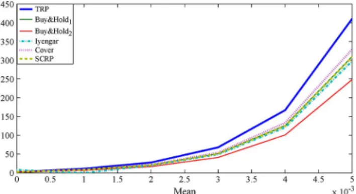
In the second example, we performed a set of simulations where each stock is generated from a log-normal distribution

such that and with

a fixed variance parameter, , as the mean increases from 0 to . We keep the difference of the means of the

two stocks constant, i.e., , to keep the ratio

Fig. 7. Performance of various portfolio investment algorithms on a Log-nor-mally simulated two-stock market under a hefty transaction cost .

Fig. 8. Performance of various portfolio investment algorithms on a Log-nor-mally simulated two-stock market under a moderate transaction cost .

Fig. 9. Performance of various portfolio investment algorithms on a Log-nor-mally simulated two-stock market under no transaction cost .

the optimal portfolio unchanged. In Fig. 4, Fig. 5 and Fig. 6, we plot the wealth growth of: the sequential TRP algorithm with the optimal parameters sequentially calculated, the Cover’s uni-versal portfolio, the Iyengar’s uniuni-versal portfolio, the SCRP al-gorithm with the suggested parameters in [16] and the two buy and hold portfolios. We present results for a hefty transaction

cost , a mild transaction cost and no

trans-action cost , respectively. As seen from the figures, the proposed TRP algorithm significantly outperforms other algo-rithms and better handle the transaction costs. As expected, for the case of small mean, i.e., where the expected gain from the stocks is close to 0, the algorithms with no rebalancing perform slightly better. However, as the mean parameter increases, the proposed TRP readily outperforms the other algorithms. Note that the TRP algorithm can better handle the transaction costs and retain its dominant performance.

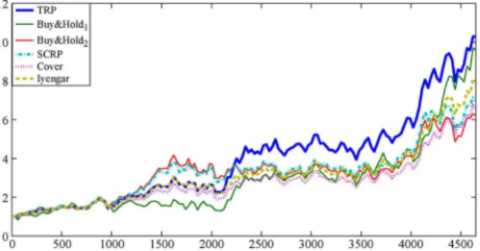
Fig. 10. Performance of various portfolio investment algorithms on Ford—MEI Corporation pair under a hefty transaction cost .

Fig. 11. Performance of various portfolio investment algorithms on Ford—MEI Corporation pair under a moderate transaction cost .

Fig. 12. Performance of various portfolio investment algorithms on Ford—MEI Corporation pair under no transaction cost .

As the next example, we apply our algorithm to historical data from [11] from the New York Stock Exchange col-lected over a 22-year period. We first apply algorithms on the “Ford—MEI Corporation” pair, which are chosen because of their volatility [13]. In Fig. 10, Fig. 11 and Fig. 12, we plot the wealth growth of: the sequential TRP algorithm with the optimal parameters sequentially calculated, the Cover’s universal portfolio, the Iyengar’s universal portfolio and the SCRP algorithm with the suggested parameters in [16]. We use the ML estimators to choose the optimal TRP as in the first set of experiments, however, since the historical data contains 5651 days we use a window of size 1000 days. Hence, the per-formance results are shown over 4651 days. As seen from the figures, the proposed TRP algorithm significantly outperforms other algorithms for this data set. Similar to the simulated data case, we investigate the performance of the TRP algorithm under different transaction costs, i.e., a hefty transaction cost

Fig. 13. Average performance of various portfolio investment algorithms on independent stock pairs under a hefty transaction cost .

Fig. 14. Average performance of various portfolio investment algorithms on independent stock pairs under a moderate transaction cost .

Fig. 15. Average performance of various portfolio investment algorithms on independent stock pairs under no transaction cost .

in Fig. 10, a moderate transaction cost in Fig. 11 and no transaction cost in Fig. 12. Comparing the results from the Fig. 10, Fig. 11 and Fig. 12, we conclude that the TRP with the optimal sequential parameter selection can better handle the transaction costs when the stocks are volatile for this experiment.

Finally, to remove any bias on a particular stock pair, we show the average performance of the TRP algorithm over randomly selected stock pairs from the historical data set from [11]. The total set includes 34 different stocks, where the Iroquois stock is removed due to its peculiar behavior. We first randomly select pairs of stocks and invest using: the sequential TRP algorithm with the sequential ML estimators, the Cover’s universal port-folio algorithm, the Iyengar’s universal portport-folio algorithm and the SCRP algorithm. The sequential selection of the optimal TRP parameters are performed similar to the previous case, i.e., we use ML estimators on an investment block of 1000 days and use the calculated optimal TRP in the next block of 1000 days.

For each stock pair, we simulate the performance of the algo-rithms over 4651 days. In Fig. 13, Fig. 14 and Fig. 15 we present the wealth achieved by these algorithms, where the results are averaged over 10 independent trials. We present the achieved wealth over random sets of stock pairs under a hefty transac-tion cost in Fig. 13, a moderate transaction cost in Fig. 14 and no transaction cost in Fig. 15. As seen from the figures, the TRP algorithm readily outperforms the other strategies under different transaction costs on this his-torical data set.

V. CONCLUSION

In this paper, we studied an important financial application, the portfolio selection problem, from a signal processing per-spective. We investigated the portfolio selection problem in i.i.d. discrete time markets having a finite number of assets, when the market levies proportional transaction fees for both buying and selling stocks. We introduced algorithms based on threshold re-balanced portfolios that achieve the maximal growth rate when the sequence of price relatives have the log-normal distribu-tion from the well-known Black-Scholes model [9]. Under this setup, we provide an iterative relation that efficiently and recur-sively calculates the expected wealth in any i.i.d. market over any investment period. The terms in this recursion are evalu-ated by a certain multivariate Gaussian integral. We then use a randomized algorithm to calculate the given integral and obtain the expected growth. This expected growth is then optimized by a brute force method to yield the optimal target portfolio and the threshold to maximize the expected wealth over any investment period. As predicted from our derivations, we significantly im-prove the achieved wealth over portfolio selection algorithms from the literature on the historical data set from [11].

REFERENCES

[1] “Special issue on signal processing methods in finance and electronic trading,” IEEE J. Sel. Top. Signal Process. [Online]. Available: http://www.signalprocessingsociety.org/uploads/special_issues_dead-lines/sp_finance.pdf

[2] “Special issue on signal processing for financial applications,” IEEE

Signal Process. Mag. [Online]. Available:

http://www.signalprocess-ingsociety.org/uploads/Publications/SPM/financial_apps.pdf [3] A. J. Bean and A. C. Singer, “Universal switching and side information

portfolios under transaction costs using factor graphs,” IEEE J. Sel.

Top. Signal Process., vol. 6, no. 4, pp. 351–365, Aug. 2012.

[4] A. Bean and A. C. Singer, “Factor graphs for universal portfolios,” in

Proc. 43rd Asilomar Conf. Signals, Syst. Comput., 2009, pp. 1375–1379.

[5] M. U. Torun, A. N. Akansu, and M. Avellaneda, “Portfolio risk in multiple frequencies,” IEEE Signal Process. Mag., vol. 28, no. 5, pp. 61–71, Sep 2011.

[6] A. Bean and A. C. Singer, “Universal switching and side informa-tion portfolios under transacinforma-tion costs using factor graphs,” in Proc.

ICASSP, 2010, pp. 1986–1989.

[7] A. Bean and A. C. Singer, “Portfolio selection via constrained sto-chastic gradients,” in Proc. Speech Signal Process., 2011, pp. 37–40. [8] M. U. Torun and A. N. Akansu, “On basic price model and volatility

in multiple frequencies,” in Proc. Speech Signal Process., June 2011, pp. 45–48.

[9] D. Luenberger, Investment Science. Oxford, U.K.: Oxford Univ. Press, 1998.

[10] H. Markowitz, “Portfolio selection,” J. Finance, vol. 7, no. 1, pp. 77–91, 1952.

[11] T. Cover, “Universal portfolios,” Math. Finance, vol. 1, pp. 1–29, Jan. 1991.

[12] T. Cover and E. Ordentlich, “Universal portfolios with side-informa-tion,” IEEE Trans. Inf. Theory, vol. 42, no. 2, pp. 348–363, 1996. [13] D. P. Helmbold, R. E. Schapire, Y. Singer, and M. K. Warmuth,

“On-line portfolio selection using multiplicative updates,” Math. Finance, vol. 8, pp. 325–347, 1998.

[14] Y. Singer, “Swithcing portfolios,” in Proc. Conf. on Uncert. Artif.

In-tell., 1998, pp. 1498–1519.

[15] V. Vovk and C. Watkins, “Universal portfolio selection,” in Proc.

COLT, 1998, pp. 12–23.

[16] S. S. Kozat and A. C. Singer, “Universal semiconstant rebalanced port-folios,” Math. Finance, vol. 21, no. 2, pp. 293–311, 2011.

[17] S. S. Kozat and A. C. Singer, “Switching strategies for sequential decision problems with multiplicative loss with application to port-folios,” IEEE Trans. Signal Process., vol. 57, no. 6, pp. 2192–2208, 2009.

[18] S. S. Kozat and A. C. Singer, “Universal switching portfolios under transaction costs,” in Proc. ICASSP, 2008, pp. 5404–5407.

[19] S. S. Kozat, A. C. Singer, and A. J. Bean, “A tree-weighting approach to sequential decision problems with multiplicative loss,” Signal

Process., vol. 92, no. 4, pp. 890–905, 2011.

[20] T. M. Cover and C. A. Thomas, Elements of Information Theory. New York, NY, USA: Wiley, 1991.

[21] A. Blum and A. Kalai, “Universal portfolios with and without transac-tion costs,” Mach. Learn., vol. 35, pp. 193–205, 1999.

[22] M. H. A. Davis and A. R. Norman, “Portfolio selection with transaction costs,” Math. Operat. Res., vol. 15, p. 676713, 1990.

[23] M. Taksar, M. Klass, and D. Assaf, “A diffusion model for optimal portfolio selection in the presence of brokerage fees,” Math. Operat.

Res., vol. 13, pp. 277–294, 1988.

[24] A. J. Morton and S. R. Pliska, “Optimal portfolio manangement with transaction costs,” Math. Finance, vol. 5, pp. 337–356, 1995. [25] M. J. P. Magill and G. M. Constantinides, “Portfolio selection with

transactions costs,” J. Econom. Theory, vol. 13, no. 2, pp. 245–263, 1976.

[26] G. Iyengar, “Discrete time growth optimal investment with costs,” 2002 [Online]. Available: http://www.ieor.columbia.edu/ gi10/Pa-pers/stochastic.pdf

[27] G. Iyengar and T. Cover, “Growths optimal investment in horse race markets with costs,” IEEE Trans. Inf. Theory, vol. 46, pp. 2675–2683, 2000.

[28] G. Iyengar, “Universal investment in markets with transaction costs,”

Math. Finance, vol. 15, no. 2, pp. 359–371, 2005.

[29] A. Borodin, R. El-Yaniv, and V. Govan, “Can we learn to beat the best stock,” J. Artif. Intell. Res., vol. 21, pp. 579–594, 2004.

[30] J. E. Cross and A. R. Barron, “Efficient universal portfolios for past dependent target classes,” Math. Finance, vol. 13, no. 2, pp. 245–276, 2003.

[31] Z. Bodie, A. Kane, and A. Marcus, Investments. New York, NY, USA: McGraw-Hill/Irwin, 2004.

[32] T. S. Ferguson, Optimal Stopping and Applications [Online]. Avail-able: http://www.math.ucla.edu/tom/Stopping/Contents.html [33] F. T. Bruss and J. B. Robertson, “Wald’s Lemma for sums of order

statistics of i.i.d. random variables,” Adv. Appl. Probabil., vol. 23, no. 3, pp. 612–623, 1991.

[34] H. Stark and J. W. Woods, Probability and Random Processes With

Ap-plications to Signal Processing. Englewood Cliffs, NJ, USA:

Pren-tice-Hall, 2001.

[35] N. H. Timm, Applied Multivariate Analysis. New York, NY, USA: Springer, 2002.

[36] A. Genz and F. Bretz, Computation of Multivariate Normal and t

Prob-abilities. New York, NY, USA: Springer, 2009.

[37] I. F. Blake and W. C. Lindsey, “Level-crossing problems for random processes,” IEEE Trans. Inf. Theory, vol. 19, no. 3, May 1973. [38] R. Richtmyer, “The evaluation of definite integrals and quasi-Monte

Carlo method based on the properties of algebraic numbers,” Los Alamos Scientif. Lab., Los Alamos, NM, USA, 1952.

[39] D. Ruppert, Statistics and Data Analysis for Financial Engineering. New York, NY, USA: Springer, 2010.

Sait Tunc received the B.S. degree in electrical and

electronics engineering from Bogazici University, Turkey, in 2010 and the M.S. degree in electrical and electronics engineering from Koc University, Turkey, in 2012.

He is currently pursuing the Ph.D. degree in in-dustrial and systems engineering at the University of Wisconsin, Madison. His research interests include signal processing, information theory, and Markov decision processes.

Mehmet Ali Donmez received the B.S. degrees from

both the Department of Electrical and Electronics Engineering and the Department of Mathematics, Bogazici University, Turkey, with honors.

He is currently pursuing the M.S. degree at the De-partment of Electrical and Electronics Engineering, Koc University, Turkey, under the supervision of Professor Suleyman S. Kozat. His current research interests are adaptive signal processing, intelligent systems, online learning, signal processing for communications, signal processing algorithms for mathematical finance, and machine learning for signal processing.

Suleyman Serdar Kozat received the B.S. degree

with full scholarship and high honors from Bilkent University, Turkey. He received the M.S. and Ph.D. degrees in electrical and computer engineering from University of Illinois at Urbana Champaign, Urbana, in 2001 and 2004, respectively.

After graduation, he joined IBM Research, T. J. Watson Research Lab, Yorktown, NY, as a Research Staff Member in the Pervasive Speech Technologies Group, where he focused on problems related to statistical signal processing and machine learning. While pursuing the Ph.D. degree, he was also working as a Research Associate at Microsoft Research, Redmond, WA, in the Cryptography and Anti-Piracy Group. He holds several patent inventions due to his research accomplishments at IBM Research and Microsoft Research. After serving as an Assistant Pro-fessor at Koc University, Turkey, he is currently an Assistant ProPro-fessor (with the Associate Professor degree from YOK) with the Electrical and Electronics Department, Bilkent University. Overall, his research interests include signal processing, adaptive filtering, sequential learning, and machine learning.

Dr. Kozat is an Associate Editor for the IEEE TRANSACTIONS ONSIGNAL

PROCESSING(and he is currently the only Associate Editor in Turkey for this top-ranking signal processing journal). He is the General Co-Chair for the IEEE Machine Learning for Signal Processing, Istanbul, 2013. He has been awarded IBM Faculty Award by IBM Research in 2011, Outstanding Faculty Award by Koc University in 2011 (granted the first time in 16 years), Outstanding Young Researcher Award by the Turkish National Academy of Sciences in 2010, ODTU Prof. Dr. Mustafa N. Parlar Research Encouragement Award in 2011 and holds Career Award by the Scientific Research Council of Turkey, 2009. He has also served on many Technical Committees of different international and national conferences and workshops. During his high school years, he won several scholarships and medals in international and national science and math competitions.