TIME SERIES PROPERTIES ADJUSTMENT
PROCESSES AND FORECASTING OF FINANCIAL RATIOS OF
FIRMS IN ISTANBUL STOCK EXCHANGE
FEYZULLAH YEĞİN
104664012
İSTANBUL BİLGİ ÜNİVERSİTESİ
SOSYAL BİLİMLER ENSTİTÜSÜ
ULUSLARARASI FİNANS
YÜKSEK LİSANS PROGRAMI
Tez Danışmanı: OKAN AYBAR
İSTANBUL 2007
TIME SERIES PROPERTIES ADJUSTMENT PROCESSES AND
FORECASTING OF FINANCIAL RATIOS OF FIRMS IN ISTANBUL STOCK
EXCHANGE
İMKB ŞİRKETLERİNİN FİNANSAL RASYOLARININ ZAMAN
SERİLERİ KULLANILARAK İNCELENMESİ VE TAHMİNİ
FEYZULLAH YEĞİN
104664012
Tez Danışmanının Adı Soyadı (İMZASI) : Okan AYBAR
Jüri Üyelerinin Adı Soyadı (İMZASI)
:
Jüri Üyelerinin Adı Soyadı (İMZASI)
:
Tezin Onaylandığı Tarih
:
Toplam Sayfa Sayısı
: 47
Anahtar
Kelimeler
(Türkçe)
Keywords
1) Finansal Rasyolar
1) Financial Ratios
2) Zaman Serileri
2) Time Series Analysis
3) ARIMA Modelleri
3) ARIMA Models
4) Stokastik
4) Stochastic Process
Special thanks to…
Okan AYBAR for encouraging me to make completion of this paper a priority and for his motivation, also for his academic support and sharing his experience with me
Prof. Dr. Oral ERDOĞAN for sharing his limited time with me, for his assistance and for his so generous patience
ABSTRACT
The objective of this study is to investigate true ARIMA models based on Aksu, Eckstein, Greene and Ronen (Aksu at. al, 1996) to forecast future values of the financial ratios of the firms which are listed in Istanbul Stock Exchange. Box-Jenkins (1976) Process of identification, estimation and diagnostic checking for the purpose of building ARIMA models for a set of selected financial ratios is used as the method. The identification tools include sample autocorrelation function (SACF) and sample partial autocorrelation function (SPACF). The patterns observed in SACF and SPACF are compared to the known patterns of theoretical ACFs and PACFs typically associated with different ARMA (p,q) (P,Q) models for making appropriate choices for p,q,P,Q (for identifying the underlying ARMA model).
The study uses the series of a total of 12 ratios and of 15 sectors. A total of 24 ARIMA models are tested with the series, beginning with ARIMA (1,0,0) to ARIMA (2,2,2) and are compared according to 8 crieterias; R – squared, adjusted R-squared, Squared Error Of Regression (SER), Sum Squared Residual (SSR), Durbin-Watson Stat (DW), Akaike Info Criterian (AIC), Schwarz Criterian (SIC) and F statistic. The models, which give the best results for most of the criterias, are selected. When there is equality for criterias; the t values, and ACF and PACF of models are evaluated. After selecting the models, in the second stage, the forecasted values of these ratios are compared with the realized values. And lastly, it is explained whether the selected ones are sufficient or not to make true forecasts; and if not how the problems with the models can be fixed.
ÖZET
Bu çalışmanın amacı; İMKB’de bulunan şirketlere ait finansal rasyoların gelecek değerlerinin tahmininde kullanılacak ARIMA modellerin bulunmasıdır. Bu amaç için Aksu, Eckstein, Greene ve Ronen’in çalışması (1996) referans noktası olarak alınmıştır. Çalışmada; Box-Jenkins (1976) methodu kullanılarak, seçilen bir finansal rasyo seti için uygun ARIMA modelleri belirlenmeye çalışılmıştır. Modeller belirlenirken, finansal rasyo serilerinin SACF ve SPACF’ları incelenmiş ve serilerin hareketleri teorik ACF ve PACF modellerinin hareketleriyle karşılaştırılarak, uygun ARMA (p,q) (P,Q) modelleri elde edilmeye çalışılmıştır.
Çalışmada toplam 12 rasyo ve 15 sektöre ait seriler incelenmiştir. ARIMA (1,0,0)’dan ARIMA (2,2,2)’ye kadar toplam 24 ARIMA modeli, sektörel bazdaki firmaların finansal rasyolarının ortalamaları alınarak elde edilen bu seriler üzerinde denenmiş ve denenen bu modeller 8 kritere göre karşılaştırılmıştır. Bu kriterler; R – squared, adjusted R-squared, Squared Error Of Regression, Sum Squared Residual, Durbin-Watson Stat, Akaike Info Criterian, Schwarz Criterian and F statistic olarak belirlenmiştir. Kriterlere göre en iyi sonuçları veren model seçilmiş, kriterler arasında eşitlik olduğunda modellerin t değerlerine, ACF ve PACF’lere bakılmıştır. Modeller seçildikten sonra rasyoların modelleme için kullanılan en son döneminden sonraki dönemin değerleriyle karşılaştırma yapılmıştır. Son olarak, seçilen modellerin doğru tahminleme yapabilmek için yeterli olup olmadığı, eğer yeterli değilse de modellerdeki problemlerin nasıl düzeltilebileceği açıklanmıştır.
TABLE OF CONTENTS
Chapter 1: Introduction ...1
1.1 Studies Relating to Financial Ratios...1
1.2 Time Series Properties, Adjustment Processes and Forecasting Of Financial Ratios; A study of Aksu at al (1996)...5
1.3 The Point Of View In This Study ...6
Chapter 2: Time Series Analysis...8
2.1 General Information...8
2.2 Stochastic Processes and Their Properties...10
2.3 Forecasting...13
Chapter 3: Research Design and Sample...17
Chapter 4: ARIMA Model Application to The Ratio Series ...19
Chapter 5: Conclusion...33
APPENDIX...35
LIST OF TABLES
Table 1: Current Ratio Models... 20
Table 2: Liquidity Ratio Models... 20
Table 3: Sales / Assets Ratio Models... 21
Table 4: Debt / Equity Ratio Models ... 21
Table 5: Leverage Ratio Models... 22
Table 6: Return On Assets Ratio Models... 22
Table 7: Return On Equity Ratio Models ... 23
Table 8: Inventory Turnover Ratio Models ... 23
Table 9: Net Profit Margin Ratio Models ... 24
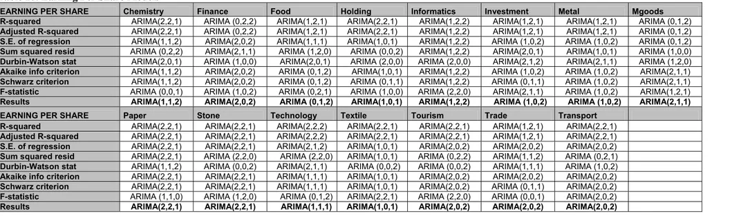
Table 10: Earning Per Share Models ... 24
Table 11: Cash / Sales Ratio Models ... 25
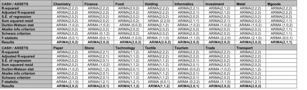
Table 12: Cash / Assets Ratio Models ... 25
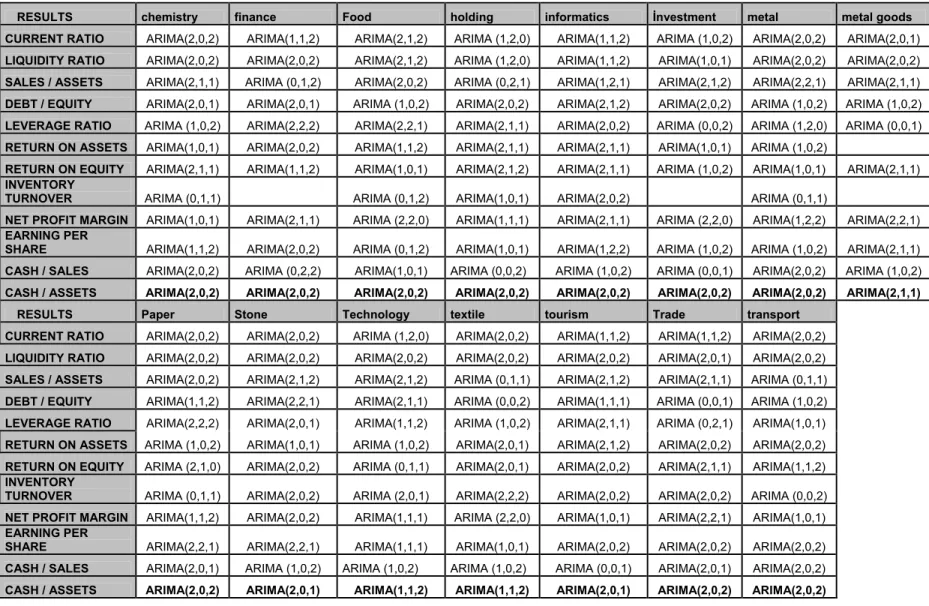
Table 13: Total Results Table ... 26
Table 14: Calculated Ratios Table ... 28
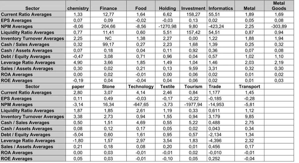
Table 15: Sectors Realized Ratio Averages in First Quarter of 2006... 29
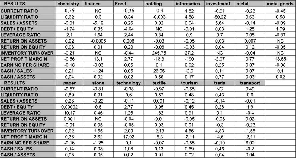
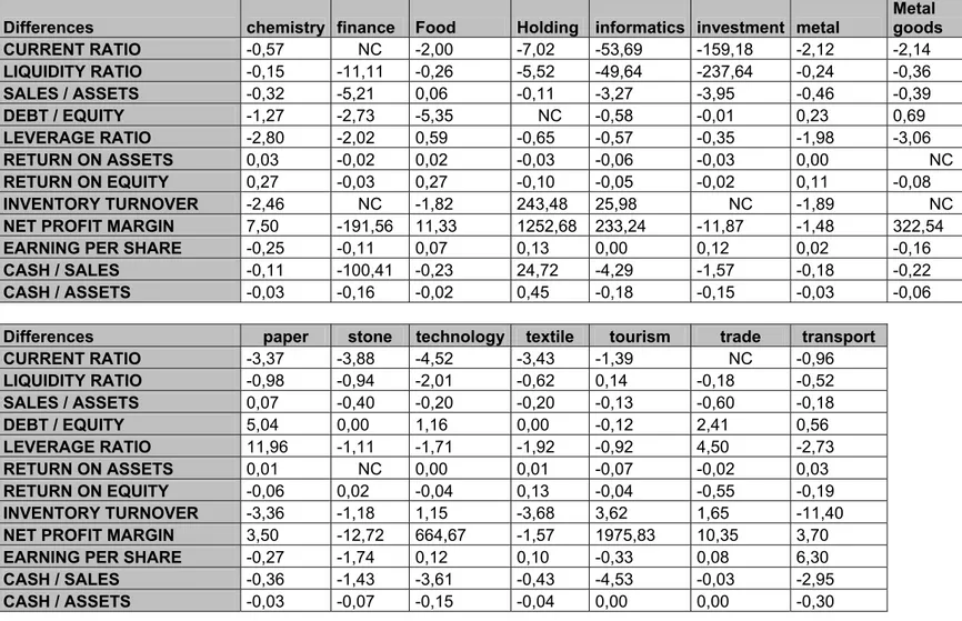
Table 16: Calculated Values – Realized Values Differences of Ratios ... 30
Abbreviations
MDA : multiple discriminant analysis ACF : autocorrelation function PACF : partial autocorrelation function SACF : sample autocorrelation function
SPACF : sample partial autocorrelation function ARMA : autoregressive moving average
ARIMA : autoregressive integrated moving average SER : squared error of regression
SSR : sum squared residual DW : durbin-watson stat AIC : akaike info criterian SIC : schwarz criterian
NYSE : New York Stock Exchange ISE : İstanbul Stock Exchange ROE : Return On Equity
ROA : Return On Assets
Chapter 1
Introduction
In this paper, it is tried to find true forecasting models of a group of financial ratios of the firms which have stocks traded in İstanbul Stock Exchange, in the light of the study Aksu at al (1996). In my knowledge such a work with financial ratios for Turkish companies has not been done until this time. Since this study is the reference point, it is thought to be useful to give some details about it. But before that study, the studies about financial ratios with using time series in the literature are summarized briefly to see which studies were done previously about financial ratios and how they approached to this topic.
1.1 Studies Relating to Financial Ratios
Studies about financial ratios previously are affected mainly about the topic that whether these ratios are effective measures of bankruptcy. The detection of company operating and financial difficulties is a subject which has been particularly susceptible to financial ratio analysis. Studies imply that a definite potential of ratios as predictors of bankruptcy. In general, ratios measuring profitability, liquidity, and solvency prevailed as the most significant indicators. But the most important question is which ratios are most important in detecting bankruptcy potential, what weighs should be attached to those selected ratios, and how should the weights be objectively established.
In this respect, Edward I.Altman (1968)1 attempted in his study to assess the quality of ratio analysis as an analytical technique. The prediction of corporate bankruptcy was used as an illustrative case. Specifically a set of financial and economic ratios were investigated in a bankruptcy prediction context wherein a multiple discriminant statistical methodology was employed.
In Altman’s study (1968), a MDA is chosen as the appropriate statistical technique, which is used to classify an observation into one of several priori groupings dependent upon the observation’s individual characteristics. The primary advantage of MDA in dealing with classification problems is the potential of analyzing the entire variable profile of the object simultaneously rather than sequentially examining its individual characteristics.
In the end of the study he states as a result that it was seen on a strictly univariate level, all of the ratios indicate higher values for the non-bankrupt firms. Also the discriminant coefficients of equation display positive signs, which is what one would expect. Therefore the greater a firm’s bankruptcy potential, the lower its discriminant score.
Based on the results, in the study it is suggested that the bankruptcy prediction model is an accurate forecaster of failure up to 2 years prior to bankruptcy and that the accruacy diminishes substantially as the lead time increases. The two most important conclusions of this trend analysis are (1) that all of the observed ratios show a deteriorating trend as bankruptcy approached, and (2) the most serious change in the majority of these ratios occured between the second and third years prior to bankruptcy.
In a similar topic; Robert O Edmister (1972)2 tried to test the usefulness of financial ratio analysis for predicting small business failure. According to him, Altman, Beaver and Blum advanced emprical research of financial analysis by applying sophisticated statistical techniques to financial data of firms that became bankrupt or otherwise failed, and firms that appeared successful. He mentioned that their research has indicated analysis of selected ratios as useful for predicting failure of medium and large asset size firms. However these and previous studies have largely ignored small businesses because of the difficulty of obtanining data.
Edmister (1972) puts several hypothesis about small firm failure prediction using financial ratios. The first hypothesis of his study is that a ratios’s level is a predictor of small business failure. For example; a firm is belived less likely to fall if its current ratio is 3/1 rather than 1/1. This hypothesis represents the use of ratios in their crudest form; no adjustment is made for variations between industries nor are the ratios compared with one another. It is based upon the theory that there are standards which transcend industry boundaries and are applicable to all firms.
The second hypothesis is that the 3 year trend of each ratio is a predictor of small business failure. Previous emprical studies considering trends have found that trends of some ratios lead to business failure. Practitioners report that businesses which are “going in the wrong direction” are viewed with greater caution than those whose trends are improving. Trend is defined as 3 consecutive years in which the ratio moves in the same direction. Fro ex: if the ratios for the last 3 years were 2/1, 3/1 and 4/1 a trend is defined; but if the ratios were 2/1, 4/1, 3/1, a trend is not considered to exist.
The third hypothesis is that the 3 year average of a ratio is a predictor of small business failure. Averaging is expected to smooth the ratios and to result in a more representative figure than that calculated from only the most recent statement. Averages are calculated for the RMA relative and SBA relative ratios to provide an index of the relative firm-to-industry position over 3 years.
The fourth hypothesis is that the combination of the industry relative trend and the industry relative level for each ratio is a predictor of small business failure. This hypothesis has not been presented in previous emprical research but is an explicit representation of the conditional nature of ratios long recognized by ratio analysts.
He concluded that to qualify his conclusions with the provisions at least 3 consecutive financial statements should be available for analysis of a small business.
In an another study about financial ratios, Edward B. Deakin (1976)3 makes some critics about Beaver and Edmister and states that applications of advanced statistical techniques to the traditional financial ratio analysis of companies has raised some questions concerning the usefulness of these ratios for persons external to the firm which are mentioned in the studies of Altman (1968), Beaver (1968), (1967), Deakin (1972), Manak and Heufner (1972), Horrigan (1967) O’Connor (1973). According to Deakin (1976) O’Connor’s findings are of particular interest since he found that financial ratios provided little or no assistance in the determination of future rate of return rankings.
According to Deakin (1976), the usefulness of studies that classify firms on the basis of accounting ratios can be enhanced considerably if the classification model can be used to make probability estimates about group membership for a particular firm. Such probability assessments are necessary inputs to expectation models. However the assignment of probabilities of group membership is still a rather inaccurate procedure.
Deakin mentions that the analysis of the raw data for 1973 showed that ten of the eleven financial accounting ratios were distributed in a manner that was significantly different from a normal distribution. As a result of this analysis it would appear that assumptions of normailty for
financial accounting ratios would not be tenable except in the case of the Total Debt / Total Assets ratio. Even for this ratio the assumption would not hold for the most recent data observations. Thus, if probability statements are to be made that are dependent upon the nature of the underlying distribution, such statements either must be based on distribution free statistics or must provide an indication of the nature of the underlying distribution of financial ratios.
In his study of quarterly earnings, Paul A. Griffin (1977)4 used the same method of Box and Jenkins (1970) as Aksu at al (1996) in his analysis for the identification of the ARIMA time series models. The models are applied to the quarterly earnings available for common stockholders series for a sample of 94 large firms listed in NYSE. The analysis suggest that there are 2 components to the quarterly earnings process: (1) a 4 period seasonal component (2) an adjacent quarter component which describes the seasonally adjusted series. Of several candidate models for this dual characterization that are examined, either a stationary first order AR or a nonstationary first order MA process adequately describes the sample. Consequently he states that it is evident that the quarterly earnings process is not a Martingale (submartingale or supermartingale) and apart from the effects of seasonality successive changes in quarterly earnings are not independent.
The results in his study are based on cross section analyses of the ACF and PACF of the quarterly earnings series. The estimated ACF is used to identify the suitable differencing required to produce stationarity in the original series. For a homogeneous stationary process, the ACF will display a tendency to decay for moderate and large lags. Moreover, since each stationary process has both unique ACF and PACF, the estimated ACF and PACF form a basis from which to infer a tentative process.
Griffin (1977) states that the aim of his study is to determine model adequacy in terms of agreement with the assumption that the estimated residuals constitute independent, identically distributed random variables with mean equal to zero and constant variance. In addition, stationarity conditions are required for an AR process of finite order, and for a MA process, the parameters must meet conditions to ensure invertibility. In the end he explains that the results of his study clearly indicate the quarterly earnings process cannot be adequately described as a random walk or a Martingale and that successive changes in quarterly earnings are independent.
1.2 Time Series Properties, Adjustment Processes and Forecasting Of Financial Ratios; A study of Aksu at al (1996)
Some past studies about financial ratios are given in the previous section. Briefly in the earlier times it is discussed whether financial ratios can be used to forecast the bankruptcy of large and small firms. Later Deakin (1976) states some doubts about the usefulness of these ratios for persons external to the firm and adds that there are other factors those should be taken into account; such as group membership for a particular firm. Lastly Griffin (1977) mentions the seasonality effect in quarterly earnings series and says that these process can not be described as a random walk or a Martingale.
In the study of Aksu at al (1996); researchers investigated the time series properties and adjustment processes of a group of financial ratios for the purpose of finding accruate forecasting models. They sought methods to identify and disentangle the permanent and transitory components of income in an effort to improve forecasting accuracy and hence equity pricing. To achieve this, ARIMA models, which removed a portion of transitory error from past earnings changes, were used. It is believed that an adequate representation of the time series of financial ratios can be obtained with ARIMA models because some of the components of financial ratios are expected to be generated by autoregressive processes. Barring extraordinary events, the assets and equity in period t+1 would be highly correlated with the assets and equity in period t. This is the result of the fact that while calculating financial ratios mostly balance sheet stock variables, which are a historical summation of accounting entries, and measurement errors are simply the sum of random shocks over history. So this means the ratios can be modeled by a moving average stochastic processes, wherein a “filter” has been applied to smooth the shocks.
Since there are facts that some components of the processes of financial ratios are autoregressive and others are moving average, the processes will be an autoregressive moving average. So the ARIMA models are used to model these financial ratios.
The ratios selected represent profitability, liquidity, cash position, turnover and capital structure. Also two deflated earnings ratios (ROE and ROA) are investigated in the study. Disaggregating data in different ways was employed to improve forecast accruacy of these ratios. For the study, the researchers used the Box-Jenkins (1976) method of identification, estimation and diagnostic checking of ARIMA models in the time series analysis and the method
of instrumental variables for the partial adjustment models. A seasonal ARIMA model takes the form:
Φp(B) ΦP (Bs) ( 1 – B) d (1-Bs) D yt = C +
θ
q (B)θQ
(Bs)at
where yt is the observed time series; B is the backshift operator such that B j yt =
y
t-j, Φp (B)and θq (B) are nonseasonal polynomials in B; ΦP (Bs) and
θQ
(Bs) are seasonal polynomials in B,where s is the seasonal period; a, is a sequence of independent, Gaussian variates distributed normal with mean 0 and variance 02; and C is a constant. The model is order (p,d,q) (P,D,Q) where p and P denote the order of the nonseasonal and seasonal autoregressive polynomials, respectively; q and Q denote the order of the nonseasonal and seasonal moving average polynomials, respectively; and d and D are the degrees of successive and seasonal differencing, respectively, required to achieve stationarity. To ensure the properties of stationarity and invertibility, all zeros of the seasonal and nonseasonal autoregressive and moving average polynomials are required to lie outside the unit circle.
1.3 The Point Of View In This Study
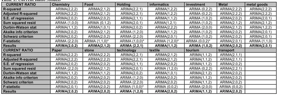
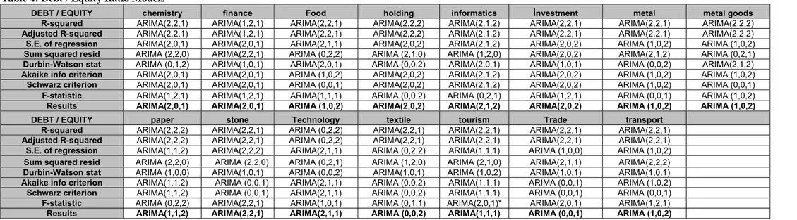
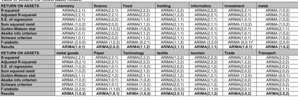
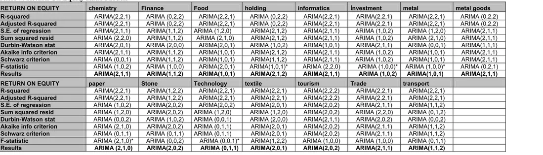
In the light of above studies the objective of this study is to find true forecasting models for financial ratios through using Box Jenkins (1976) Procedure5. The data set is the financial ratios of firms in Istanbul Stock Exchange. For the period of 1996 – 2005 the quarterly data of 156 firms in 15 sectors are used. For each ratio, sector averages for each quarter are found and time series with 40 values, for each ratio, are obtained. Next, using E-Views program, 24 ARIMA models are tested with these series and they are evaluated according to 8 criterias to get a true forecasting model. For example for Current Ratio; after selecting the best ARIMA model with R-squared criteria, this model is placed to Table 1 (page 26) as ARIMA (2,2,2). The table is filled for all sectors and for all criterians like this. When there is more than one model which is good for some criterias and the other for other criterias, I took the model which give best results for most of the criterias or which give the better result for some criterias such as R-squared.
Next, a second table is filled in the same way for liquidity ratio. A total of 12 tables are evaluated and filled like this and the summary of models for all ratios and all sectors is given in Table 13 (page 32). After deciding the models, they are used to forecast next period values (page 34, Table 14). And then the forecasted values are compared with the real ones (page 36).
The models selected through this way in this study are also decided with the diagnostic checking of the ACF and PACF of the financial ratio series. The stationarity of the series are checked and if they are not stationary, the differencing method is used until a stationary series is achieved. And it is after achieving a stationary series, a suitable ARIMA model is tried to find.
According to the results of this study, the models are found to be weak to make healthy estimates, although in some sectors there are little differences of forecasted values with the real values. There may be many reasons for this result but the most important one is thought to be the seasonality effect. Since the ratios are quarterly, they are correlated with the values 4 terms past and later. So the seasonality effect should be removed to get better results. This effect can be removed by using a seasonal ARIMA model ARMA (p,q) (P,Q)6 as done in the study of Aksu at all (1996).
In the study while obtaining sector averages, the simple average of ratios are taken into account. But although the firms are all listed in İstanbul Stock Exchange, they are different in size and their effect is different to their sector. So a weighted average of firms may be a better way to get the sector average financial ratios. It will be more helpful for better forecasts. And lastly because the firm number in ISE is restricted, the models for the study might be selected with not enough data set and so some insufficient models might be selected. For later studies, increasing number of firms in data set will fix such deficiencies.
This is the general outline of this study and the organization of the paper is as follows: In section 2, a brief information about time series analysis is given; in section 3, the detailed information about the study and methodology used in the paper, is given; in section 4; the application of ARIMA models to the series is given and the results are placed and in section 5; the conclusion is given.
Chapter 2
Time Series Analysis
72.1 General Information
Statistical techniques for analysing time series range from relatively straightforward descriptive methods to sophisticated inferiential techniques. Descriptive methods should generally be tried before attempting more complicated procedures, because they can be vital in “cleaning” the data, and then getting a “feel” for them, before trying to generate ideas as regards a suitable model.
It may be expected as a beginning to deal with summary statistics such as sample mean, standard deviation etc. But time series analysis is different. If a time series contains trend, seasonality or some other systematic component, the usual summary statistics can be seriously misleading and should not be calculated.
Traditional methods of time-series analysis are mainly concerned with decomposing the variation in a series into components representing trend, seasonal variation and other cyclic changes. Any remaining variation is attributed to “irregular” fluctuations.
The first and most important step in any time series analysis is to plot the observations against time. This graph, called a time plot, will show up important features of the series such as trend, seasonality, outliers and discontinuities.
Plotting the data may suggest that it is sensible to consider transforming them, for example, by taking logarithms or square roots. This is made to stabilize the variance (in particular the standard deviation is directly proportional to the mean), to make the seasonal effect additive (to transform the data so as to make the seasonal effect constant from year to year) and to make the data normally distributed.
The simplest type of trend is the familiar “linear trend + noise”, for which the observation at time t is a random variable Xt given by;
Xt = α + βt + εt
7 This part is prepared by using the writers’ own class notes, Tyran Michael’s “Handbook of Business and Financial Ratios” and Chris Chatfield’s “The Analysis of Time Series: An Introduction” 6.th edition
where α , β are constants and εt denotes a random error term with zero mean. It is sometimes
prefered to describe the slope β as the trend, so that trend is the change in the mean level per unit time.
The analysis of a time series that exhibit trend depends on whether one wants to (1) measure the trend and / or (2) remove the trend in order to analyze local fluctuations. It also depends on whether the data exhibit seasonality. With seasonal data it is a good idea to start by calculating successive yearly averages, as these will provide a simple description of the underlying trend. There are more than one approaches to describe a trend such as curve fitting, filtering and differencing. I will use here the differencing method, which is particularly useful for removing a trend and is simply to difference a given time series until it becomes stationary8. This method is an integral part of the so-called Box-Jenkins procedure. For non seasonal data, first order differencing is usually sufficient to attain apparent stationarity. Here a new series (y2,…,yn) is formed from the
original observed series say (X1,…,Xn) by yt = xt – xt-1 = ∆xt for t = 2,3,…,n.
Occasionaly second order differencing is required using the operator ∆2, where; ∆2 xt = ∆ xt – ∆ xt-1 = xt – 2xt - 1 + xt – 2
First differencing is widely used and often works well. For example, Franses and Kleibergen (1996) show that better out-of-sample forecasts are usually obtained with economic data by using first differences rather than fitting a deterninistic trend.
An important guide to the properties of a time series is provided by a series of quantities called the sample autocorrelation coefficients. They measure the correlation between observations at different distances apart and provide useful descriptive information.
The formula to calculate autocorrelation coefficient is: R1 = (Σt=1, N-1 (xt - x*) (xt+1 - x*)) / Σt=1, N (xt - x*)2
and in a similar way we can find the correlation between observations that are k steps apart;
8 Stationarity: Broadly speaking a time series is said to be stationary if there is no systematic change in mean (no trend), if there is no systematic change in variance and if strictly periodic variations have been removed.
Rk = (Σt=1, N-k (xt - x*) (xt+k - x*)) / Σt=1, N (xt - x*)2
And the autocovariance coefficients (ck) is calculated by the formula;
Ck = 1 / N (Σt=1, N-k (xt – x*) (xt+k – x*)). This is the autocovariance coefficient at lag k.
So Rk = Ck / C0 for k = 1,2,…, M where M < N
If a time series contains a trend, then the values of Rk will not come down to zero except for
very large values of the lag. This is because an observation on the one side of the overall mean tends to be followed by a large number of further observations on the same side of the mean because of the trend. In fact the sample ACF (Rk) is only meaningful for data from a stationary
time series model and so any trend should be removed before calculating (Rk).
Outliers: If a time series contains one or more outliers, the correlogram may be seriously affected and it may be advisable to adjust outliers in some way before starting the formal analysis. 2.2 Stochastic Processes and Their Properties
Most physical processes in the real world involve a random element in their structure and a stochastic process can be described as `a statistical phenomenon that evolves in time according to probabilistic laws. Mathematically, a stochastic process may be defined as a collection of random variables that are ordered in time and defined at a set of time points, which may be continuous or discrete.
Many models for stochastic processes are expressed by means of an algebric formula relating the random variable at time t to past values of the process, together with values of an unobservable “error” process. A simpler way is to give the moments of the process, particularly the first and the second moments that are called the mean and autocovariance function (ACF).
Mean: µ = E (x(t)) Variance: ξ2 = Var (x(t))
Autocovariance : The variance function alone is not enough to specify the second moments of a sequence of random variables. Auto covariance function is defined as: ACF γ (t1, t2) =
E ((X(t1) - µ(t1)) (X (t2) - µ(t2))9
9 The variance function is a special case of the ACF when t 1 = t2.
Fitting Time Series Models In The Time Domain
Having plotted the correlogram we can check for randomness by plotting approximate 95% confidence limits at ± 2 / √ N. Observed values of Rk which fall outside these limits are
“significantly” different from zero at the 5% level. However when interpreting a correlogram, it must be remembered that the overall probability of getting at least one coefficient outside these limits, given that the data really are random, increases with the number of coefficients plotted. A single coefficient just outside the null 95% confidence limits may be ignored, but 2 or 3 values well outside the “null” limits will be taken to indicate non-randomness. A single “significant” coefficient at a lag which has some physical interpretation, such as lag 1 or a lag corresponding to seasonal variation, will also provide plausible evidence of non-randomness.
The correlogram is helpful in trying to identify a suitable class of models for a given time series and in particular for selecting the most appropriate type of ARIMA models. A correlogram, where the values of Rk do not come down to zero reasonably quickly, indicates non – stationarity
and so the series needs to be differenced. For stationary series, the correlogram is compared with the theoretical ACFs of different ARMA processes in order to choose the one which seems to be the “best” representation. For example the ACF of an MA(q) process is easy to recognize as it “cuts off” at lag q. But while selecting models, I also take care the statistical values of each model such as R-square, AIC, SIC and Durbin-Watson.
Estimating The Mean
It is already noted that the sample mean is a potentially misleading summary statistic unless all systematic components have been removed. Thus the sample mean should only be considered as a summary statistic for data thought to have come from a stationary process.
Fitting the AR process
Having estimated the ACF of a given time series, we should have some idea as to which stochastic process will provide a suitable model. If an AR process is thought to be appropriate, there are two related questions:
1- What is the order of the process?
Residual Analysis
When a model has been fitted to a time series, it is advisable to check that the model really does provide an adequate description of the data. As with most statistical models, this is usually done by looking at the residuals;
Residual = observation – fitted value
For a univariate time series model, the fitted value is the one step ahead forecast so that the residual is the one step ahead forecast error. For ex: for the AR(1) model,
Xt = α Xt-1 + Zt
where α is estimated by least squares, the fitted value at time t is α* Xt-1 so that the residual
corresponding to the observed value, Xt, is
Zt* = Xt – α Xt-1
If we have a “good” model, then we expect the residuals to be “random” and “close to zero” and model validation usually consists of plotting residuals in various ways to see whether this is the case. With time series models we have the added feature that the residuals are ordered in time and it is natural to treat them as a time series.
Two obvious steps are to plot the residuals as a time plot, and to calculate the correlogram of the residuals. The time plot will reveal any outliers and any obvious autocorrelation or cyclic effects. The correlogram of the residuals will enable autocorrelation effects to be examined more closely. Let Rz,k denote the autocorrelation coefficient at lag k of the residuals (Zt). If we could fit
the true model with the correct model parameter values, than the true errors (Zt) form a purely
random process and their correlogram is such that each autocorrelation coefficient is approximately normally distributed., with mean 0 and variance 1/ N, for reasonably large values of N. If we fit the wrong form of model, then the distribution of residual autocorrelations will be quite different, and we hope to get some “significant” values so that the wrong model is rejected. 1 / √ N supplies an upper bound for the standard error of the residual autocorrelations, so that values, which lie outside the range ±2√ N are significantly different from zero at the 5% level and give evidence that the wrong form of model has been fitted.
Finding a suitable model for a given time series depends on various considerations, including the properties of the series as assessed by a visual examination of the data, the number of observations available, the context and the way the model is to be used.
2.3 Forecasting
Let’s we have an observed time series x1, x2, x3,…,xn. Then the basic problem is to estimate
future values such as xn+h where the integer h is called the lead time or forecasting horizon.
Forecasts are conditional statements about the future based on specific assumptions. Thus forecasts are not sacred and the analyst should always be prepared to modify them as necessary in the light of any external information.
There are two types of forecasts (except the subjuctive one which is based on own experience) which are univariate and multivariate.
Univariate: Forecasts of a given variable are based on a model fitted only to present and past observations of a given time series, so that xn+h depends only on the values of xn, xn-1 xn-2,… possibly
augmented by a simple function of time, such as a global linear trend. this would mean, for example, that univariate forecasts of the future sales of a given product would be based entirely on past sales, and would not take account of other economic factors.
Exponential Smoothing: Given a non-seasonal time series, say x1, x2, …,xn with no
systematic trend, it is natural to forecast xn+1 by means of a weighted sum of the past observations:
xn+1 = C0Xn + C1Xn-1 +C2Xn-2 +…
where the (Ci) are weights. It seems sensible to give more weight to recent observations and
less weight to observations further in the past. An intuitively appealing set of weights are geometric weights, which decrease by a constant ratio for every unit increase in the lag. So Ci = α
(1 - α)i i = 0, 1, 2, …
where α is constant such that 0 < α < 1. So the equation becomes xn+1 = α Xn + α (1 - α)Xn-1 +α (1 - α)2 Xn-2 +…
This procedure is called simple exponential smoothing. The adjective “exponential” arises from the fact that the geometric weights lie on an exponential curve.
Although intuitively appealing, it is natural to ask when SES is a “good” method to use. It can be shown that SES is optimal if the underlying model for the time series is given by
Xt = µ + α Σ Zj + Zt
where (Zt) denotes a purely random process. This infinite order MA process is
non-stationary, but the first differences (Xt+1 - Xt) form a stationary first order MA process. Thus Xt is
an ARIMA process of order (0,1,1).
The value of the smoothing constant α depends on the properties of the given time series. Values between 0.1 and 0.3 are commonly used and produce a forecast that depends on a large number of past observations.
Multivariate:Forecasts of a given variable depend at least partly on values of one or more additional series, called predictor or explanatory variables. For example, sales forecasts may depend on stocks and / or on economic indices.
Box – Jenkins Procedure
In order to identify an appropriate ARIMA model, the first step in the Box – Jenkins procedure is to difference the data until they are stationary. This is achieved by examining the correlograms of various differenced series until one is found that comes down to zero “fairly quickly” and from which any seasonal cyclic effect has been largely removed, although there could still be some spikes at the seasonal lags s, 2s and so on, where s is the number of observations per year. For non seasonal data, first order differencing is usually sufficient to attain stationarity. For three monthly data, the operator ∆4 is often used if the seasonal effect is additive, while the
operator ∆24 may be used if the seasonal effect is multiplicative.
For non seasonal data, an ARMA model can be fitted to (Wt). If the data are seasonal than an
ARIMA model may be fitted. For both seasonal and non seasonal data the adequacy of the fitted model should be checked by what Box and Jenkins call “diagnostic checking”. This essentially consists of examining the residuals from the fitted model to see whether there is any evidence of
non-randomness. The correlogram of the residuals is calculated and we can then see how many coefficients are significantly different from zero and whether any further terms are indicated for the ARIMA model. If the fitted model appears to be inadequate, then alternative ARIMA models may be tried until a satisfactory one is found.
When a satisfactory model is found, forecasts may readily be computed. Given data up to time N, these forecasts will involve the observations and the fitted residuals up to and including time N. The minimum mean square error forecast of Xn+h at time N is the conditional expectation
of Xn+h at time N, namely X*N (h) = E (Xn+h / Xn, Xn-1,…). In evaluating this conditional
expectation, we use the fact that the “best” forecast of all future Z is simply zero (or more formally that the conditional expectation of Zn+h, given data up to time N, is zero for all h>0). Box et al
(1994) describe three general approaches to computing forecasts. (1) Using the model equation directly
Point forecasts are usually computed most easily directly from the ARIMA model equation, which Box et al. (1994) call the difference equation form. Assuming that the model equation is known exactly, then X*N (h) is obtained from the model equation by replacing;
(i) future values of Z by zero
(ii) future values of X by their conditional expectation
(iii) present and past values of X and Z by their observed values (2) Using the ψ weights
An ARMA model can be rewritten as an infinite-order MA process and the resulting ψ weights could also be used to compute forecasts, but are primarily helpful for calculating forecast error variances. Since;
Xn+h = Zn+h + ψ Zn+h-1 + …
and future Zs are unknown at time N, it is clear that X*N (h) is equal to Σ∞ j=0 ψh+j zn-j (since
future Zs cannot be included). Thus the h-steps ahead forecast error is (Zn+h +ψ1Zn+h-1+…+ ψh-1 Zn+1 ). Hence the variance of the h-steps ahead forecast error is
(3) Using the П weights
An ARMA model can also be rewritten as an infinite order AR process and the resulting П weights can also be used for compute point forecasts. Since
Xn+h = П1Xn+h-1+…+ П h Xn + …+ Zn+h
it is clear that X*N (h) is given by
X*N (h) = П1 X*N (h-1) + П2 X*N (h-2) +…+ Пh+1 Xn-1
These forecasts can be computed recursively, replacing future values of X with predicted values as necessary.
Chapter 3
Research Design and Sample
Financial ratios series which are composed of quarterly data are used in this study. The quarterly data are interested in an effort to reduce the potential confounding that may result from structural changes that are likely to occur over long periods of time and to reduce the inefficiencies caused by the use of an inadeqaute number of observations for time series analysis. The time series analysis that are used for the financial ratios here, belong to the general class of linear stochastic autoregressive integrated moving average (ARIMA) models. This is because, some of the components of financial ratios (e.g., assets, equity and inventory) are expected to be generated by autoregressive processes and other by moving average. The assets and equity in period t+1 would be highly correlated with the assets and equity in period t. In its work Lee (1984) notes that most financial ratios use balance sheet stock variables, which are a historical summation of accounting entries, and measurement errors are simply the summation of the random shocks over this history. Consequently, the ratios can be modeled as if generated by moving average stochastic processes, wherein taking difference has been applied to smooth the shocks those entering the system.
If some components of a process are autoregressive and others are moving average, the process will be an autoregressive moving average (ARMA). In the study such models are used in modeling the financial ratios, because there are good theoretical reasons for believing that mixed models (ARMA) are most likely to be found in the real world especially in business and economics. But through diagnostic checking, it is found that some financial ratio series are not stationary. So to achieve a stationary series, the differencing method is employed and so here Autoregressive Integrated Moving Average (ARIMA) models are taken interest, instead of simple ARMA models10.
The financial ratios those are engaged, with their categories are given below:
Profitability:
Net Profit Margin (PRF) Return On Assets (ROA) Return On Equity (ROE) Earning Per Share (EPS)
Cash Position:
Cash / Sales (CS) Cash / Assets (CA)
Liquidity:
Current Ratio (CR) Liquidity Ratio (LR)
Turnover:
Sales / Assets (SA) COGS / Inventory (IT)
Capital Structure:
Liabilities / Equity (D/E) Assets / Common Equity (LR)
The following industries are analyzed seperately:
Chemistry, Finance, Food, Holding, Informatics, Investment, Metal, Metal Goods, Paper, Stone, Technology, Textile, Tourism, Trade, Transport. In choosing the sectors for the data set, the ones with the most number of firms are taken care.
The quarterly data are obtained from FINNET. The time period is between the first quarter of 1996 and with the fourth quarter of 2005. For a firm to be included in the sample, it had to have uninterrupted data for the entire period. A total of 156 firms are included to the sample. The most crowded sectors were stone with 24 firms, textile with 22 firms and chemistry and metal goods sector with 20 firms. The data of each firm in a sector is summed and an average value is taken to be used in time series analysis. This is the series that 24 ARIMA models are used to find a true forecasting model.
Chapter 4:
ARIMA Model Application to The Ratio Series
In the study of Aksu at all (1996); the Box-Jenkins (1976) method of identification, estimation and diagnostic checking is used for the purpose of building firm-specific and global ARIMA models. In this study the same method is also used to build true ARIMA models for financial ratios. An ARIMA model is in the form;
Xt = α Xt-1 + α2 Xt-2 +…+β
εt
+ β2εt-2 +β3 εt-3+…The model is an order (p,d,q) where p denotes the order of the autoregressive polynomials, q denotes the order of the moving average polynomials and d is the degree of successive and seasonal differencing required to achieve stationarity. To ensure the properties of stationarity and invertibility all zeros of the seasonal and nonseasonal autoregressive and moving average polynomials are required to lie outside the unit circle.
The way which is followed in this study can be summarized like this: simple average of financial ratios of firms in each sector is calculated and data series for each ratio, with 40 values, are obtained. Then via using E-views program, 24 ARIMA models are tested to determine which one is the best to model the series, according to 8 criterias. Generally not a model gives best results for each of 8 criterias; some models were best in R-square but lower in AIC and SIC or F values and vice versa. So, the model which give better results for most criterias, is selected to forecast the future value of the ratio. For other cases, for example when there is equality of criterias correlegrams and t values for coefficients are checked. Then a last decision to obtain a possible parsimonuos model is given. Later, the forecasted values which are calculated using these models compared the real values of next term (here, first quarter of 2006) and checked if the residuals are normally distributed. Below; the selected models per ratio and sector are given.
Table 1: Current Ratio Models
CURRENT RATIO Chemistry Food Holding informatics investment Metal metal goods R-squared ARIMA(2,2,2) ARIMA(2,1,2) ARIMA(2,2,1) ARIMA(1,2,2) ARIMA (0,2,2) ARIMA(2,2,2) ARIMA(2,2,2) Adjusted R-squared ARIMA(2,2,2) ARIMA(2,1,2) ARIMA(2,2,1) ARIMA(1,2,2) ARIMA (0,2,2) ARIMA(2,2,2) ARIMA(2,2,2) S.E. of regression ARIMA(2,0,2) ARIMA(2,0,2) ARIMA(2,1,1) ARIMA(1,1,2) ARIMA (1,0,2) ARIMA(2,0,2) ARIMA(2,0,1) Sum squared resid ARIMA (1,0,0) ARIMA (0,1,2) ARIMA(2,0,1) ARIMA(1,2,1) ARIMA (1,0,2) ARIMA(2,1,2) ARIMA(2,1,2) Durbin-Watson stat ARIMA(1,1,2) ARIMA(1,0,1) ARIMA(2,0,2) ARIMA(2,2,2) ARIMA (2,0,0) ARIMA(2,1,2) ARIMA(1,2,2) Akaike info criterion ARIMA(2,0,2) ARIMA(2,1,2) ARIMA (1,2,0) ARIMA(1,1,2) ARIMA (1,0,2) ARIMA(2,0,2) ARIMA(2,0,1) Schwarz criterion ARIMA(2,0,2) ARIMA(2,0,2) ARIMA (2,2,0) ARIMA(2,0,1) ARIMA (1,0,2) ARIMA(2,0,2) ARIMA(2,0,1) F-statistic ARIMA (2,2,0) ARIMA (1,1,0)* ARIMA (1,0,0)* ARIMA (1,2,0)* ARIMA (0,0,2)* ARIMA(2,0,1) ARIMA (1,1,0) Results ARIMA(2,0,2) ARIMA(2,1,2) ARIMA (2,2,1) ARIMA(1,1,2) ARIMA (1,0,2) ARIMA(2,0,2) ARIMA(2,0,1)
CURRENT RATIO Paper stone technology textile tourism transport
R-squared ARIMA(2,2,2) ARIMA(2,2,2) ARIMA(2,2,1) ARIMA(2,1,2) ARIMA(1,1,2) ARIMA(2,1,1) Adjusted R-squared ARIMA(2,2,2) ARIMA(2,2,2) ARIMA(2,2,1) ARIMA(2,1,2) ARIMA(1,1,2) ARIMA(2,1,1) S.E. of regression ARIMA(2,0,2) ARIMA(2,0,2) ARIMA(2,1,1) ARIMA(2,0,2) ARIMA(1,1,2) ARIMA(2,0,2)
Sum squared resid ARIMA (2,2,0) ARIMA(2,1,2) ARIMA(2,0,1) ARIMA (1,2,0) ARIMA (0,2,2) ARIMA(2,2,1) Durbin-Watson stat ARIMA(1,1,2) ARIMA(1,1,2) ARIMA(2,0,2) ARIMA(1,0,1) ARIMA(2,1,2) ARIMA(2,0,2)
Akaike info criterion ARIMA(2,0,2) ARIMA(2,0,2) ARIMA (1,2,0) ARIMA(2,0,2) ARIMA(1,1,2) ARIMA(2,0,2) Schwarz criterion ARIMA(2,0,2) ARIMA(2,0,2) ARIMA (2,2,0) ARIMA(2,0,2) ARIMA(1,1,2) ARIMA(2,0,2) F-statistic ARIMA(2,0,1) ARIMA(2,0,2) ARIMA (1,0,0)* ARIMA (0,0,2) ARIMA (2,0,0) ARIMA (0,0,2)
Results ARIMA(2,0,2) ARIMA(2,0,2) ARIMA (1,2,0) ARIMA(2,0,2) ARIMA(1,1,2) ARIMA(2,0,2)
Table 2: Liquidity Ratio Models
LIQUIDITY RATIO Chemistry finance Food holding informatics İnvestment metal metal goods R-squared ARIMA(2,2,2) ARIMA (0,2,2) ARIMA(2,1,2) ARIMA(2,2,1) ARIMA(2,2,2) ARIMA(2,2,2) ARIMA(2,2,2) ARIMA(2,2,2) Adjusted R-squared ARIMA(2,2,2) ARIMA (0,2,2) ARIMA(2,1,2) ARIMA(2,2,1) ARIMA(2,2,2) ARIMA(2,2,2) ARIMA(2,2,2) ARIMA(2,2,2) S.E. of regression ARIMA(2,0,2) ARIMA(2,0,2) ARIMA(2,1,2) ARIMA(2,1,1) ARIMA (1,2,0) ARIMA(1,0,1) ARIMA(2,0,2) ARIMA(2,0,2) Sum squared resid ARIMA(2,2,1) ARIMA (0,1,1) ARIMA(2,1,2) ARIMA(2,0,1) ARIMA(2,0,1) ARIMA(1,0,1) ARIMA (0,2,1) ARIMA(1,2,2) Durbin-Watson stat ARIMA(1,1,2) ARIMA (1,0,0) ARIMA (1,0,2) ARIMA (1,0,2) ARIMA (2,0,0) ARIMA (2,0,0) ARIMA(1,2,2) ARIMA(1,2,2) Akaike info criterion ARIMA(2,0,2) ARIMA(2,0,2) ARIMA(2,0,2) ARIMA (1,2,0) ARIMA(1,1,2) ARIMA(1,0,1) ARIMA(2,0,2) ARIMA(2,0,2) Schwarz criterion ARIMA(2,0,2) ARIMA(2,0,2) ARIMA(2,0,2) ARIMA (2,2,0) ARIMA(1,1,2) ARIMA(1,0,1) ARIMA(2,0,2) ARIMA(2,0,2) F-statistic ARIMA (1,1,0)* ARIMA(2,0,2) ARIMA(1,0,1) ARIMA (1,0,0)* ARIMA (1,0,0) ARIMA (2,0,0)* ARIMA (1,1,0)* ARIMA (1,1,0) Results ARIMA(2,0,2) ARIMA(2,0,2) ARIMA(2,1,2) ARIMA (1,2,0) ARIMA(1,1,2) ARIMA(1,0,1) ARIMA(2,0,2) ARIMA(2,0,2)
LIQUIDITY RATIO Paper stone technology textile tourism Trade transport
R-squared ARIMA (0,2,2) ARIMA(2,2,2) ARIMA(2,1,1) ARIMA(2,2,2) ARIMA(1,2,1) ARIMA(2,1,2) ARIMA(2,2,1) Adjusted R-squared ARIMA (0,2,2) ARIMA(2,2,2) ARIMA(2,1,1) ARIMA(2,2,2) ARIMA(1,2,1) ARIMA(2,1,2) ARIMA(2,2,1) S.E. of regression ARIMA(2,0,2) ARIMA(2,0,2) ARIMA(2,0,2) ARIMA(2,0,2) ARIMA(2,0,2) ARIMA(2,0,1) ARIMA(2,0,2) Sum squared resid ARIMA (1,0,0) ARIMA(1,2,1) ARIMA(1,2,1) ARIMA(2,2,1) ARIMA (2,2,0) ARIMA (0,2,2) ARIMA (2,1,0) Durbin-Watson stat ARIMA(1,1,2) ARIMA(1,1,2) ARIMA (1,0,2) ARIMA(1,0,1) ARIMA (0,0,2) ARIMA (1,0,0) ARIMA(2,1,2) Akaike info criterion ARIMA(2,0,2) ARIMA(2,0,2) ARIMA(2,0,2) ARIMA(2,0,2) ARIMA(2,0,2) ARIMA(2,0,1) ARIMA(2,0,2) Schwarz criterion ARIMA(2,0,2) ARIMA(2,0,2) ARIMA(2,0,2) ARIMA(2,0,2) ARIMA(2,0,2) ARIMA(2,0,1) ARIMA(2,0,2) F-statistic ARIMA (0,0,2) ARIMA(2,0,2) ARIMA (2,2,0) ARIMA(1,0,1) ARIMA (0,0,2)* ARIMA(1,1,2) ARIMA (0,0,1)* Results ARIMA(2,0,2) ARIMA(2,0,2) ARIMA(2,0,2) ARIMA(2,0,2) ARIMA(2,0,2) ARIMA(2,0,1) ARIMA(2,0,2)
Table 3: Sales / Assets Ratio Models
SALES / ASSETS chemistry Finance Food holding informatics İnvestment metal metal goods
R-squared ARIMA(2,2,2) ARIMA(1,2,2) ARIMA(2,2,2) ARIMA (0,2,1) ARIMA(1,2,1) ARIMA(2,2,2) ARIMA(2,2,1) ARIMA(2,2,1) Adjusted R-squared ARIMA(2,2,2) ARIMA(1,2,2) ARIMA(2,2,2) ARIMA (0,2,1) ARIMA(1,2,1) ARIMA(2,2,2) ARIMA(2,2,1) ARIMA(2,2,1) S.E. of regression ARIMA(2,1,2) ARIMA(2,1,1) ARIMA(2,0,2) ARIMA (0,2,1) ARIMA(1,2,1) ARIMA(2,1,2) ARIMA(2,2,1) ARIMA(2,1,1) Sum squared resid ARIMA(2,1,2) ARIMA (1,2,0) ARIMA(2,0,2) ARIMA (0,2,1) ARIMA(1,2,1) ARIMA (1,0,0) ARIMA(2,2,1) ARIMA(2,1,1) Durbin-Watson stat ARIMA (1,1,0) ARIMA(1,1,2) ARIMA(1,1,1) ARIMA (0,1,1) ARIMA (2,2,0) ARIMA(2,0,1) ARIMA (0,1,2) ARIMA(2,1,2) Akaike info criterion ARIMA(2,1,1) ARIMA (0,1,2) ARIMA(2,0,2) ARIMA (0,2,1) ARIMA (0,2,1) ARIMA(2,1,2) ARIMA (0,1,2) ARIMA(2,1,1) Schwarz criterion ARIMA(2,1,1) ARIMA (0,1,2) ARIMA(1,0,1) ARIMA (0,2,1) ARIMA (0,2,1) ARIMA(2,1,2) ARIMA (0,1,2) ARIMA(2,1,1) F-statistic ARIMA(1,1,2) ARIMA (1,1,0)* ARIMA (1,1,0) ARIMA (0,2,1) ARIMA(1,1,2)* ARIMA (1,0,0)* ARIMA (0,1,2) ARIMA(1,1,2) Results ARIMA(2,1,1) ARIMA (0,1,2) ARIMA(2,0,2) ARIMA (0,2,1) ARIMA(1,2,1) ARIMA(2,1,2) ARIMA(2,2,1) ARIMA(2,1,1)
SALES / ASSETS paper Stone Technology textile tourism Trade transport
R-squared ARIMA (0,2,2) ARIMA(2,2,1) ARIMA(1,2,2) ARIMA(2,2,1) ARIMA(2,2,2) ARIMA(2,2,1) ARIMA(2,2,1) Adjusted R-squared ARIMA (0,2,2) ARIMA(2,2,1) ARIMA(1,2,2) ARIMA(2,2,1) ARIMA(2,2,2) ARIMA(2,2,1) ARIMA(2,2,1)
S.E. of regression ARIMA(2,0,2) ARIMA(2,1,2) ARIMA(2,1,2) ARIMA(2,0,2) ARIMA(2,1,2) ARIMA(2,1,1) ARIMA (0,1,1) Sum squared resid ARIMA(2,0,2) ARIMA(2,1,2) ARIMA(2,1,2) ARIMA(2,0,2) ARIMA(2,1,2) ARIMA(2,1,2) ARIMA (0,1,1) Durbin-Watson stat ARIMA (1,1,0) ARIMA(1,0,1) ARIMA(2,1,1) ARIMA(2,0,1) ARIMA (0,0,1) ARIMA (1,0,0) ARIMA(1,0,1) Akaike info criterion ARIMA(2,0,2) ARIMA(2,1,2) ARIMA(2,1,2) ARIMA(1,0,1) ARIMA(2,1,2) ARIMA(2,1,1) ARIMA (0,1,1) Schwarz criterion ARIMA(2,0,2) ARIMA(2,1,2) ARIMA(2,1,2) ARIMA (0,1,1) ARIMA(2,1,2) ARIMA(2,1,1) ARIMA (0,1,1) F-statistic ARIMA(1,1,2) ARIMA (1,1,0) ARIMA (0,2,2) ARIMA (1,0,2) ARIMA (1,1,0) ARIMA(1,0,1) ARIMA(2,1,1) Results ARIMA(2,0,2) ARIMA(2,1,2) ARIMA(2,1,2) ARIMA (0,1,1) ARIMA(2,1,2) ARIMA(2,1,1) ARIMA (0,1,1)
Table 4: Debt / Equity Ratio Models
DEBT / EQUITY chemistry finance Food holding informatics İnvestment metal metal goods
R-squared ARIMA(2,2,1) ARIMA(1,2,1) ARIMA(2,2,1) ARIMA(2,2,2) ARIMA(2,1,2) ARIMA(2,2,1) ARIMA(2,2,1) ARIMA(2,2,2) Adjusted R-squared ARIMA(2,2,1) ARIMA(1,2,1) ARIMA(2,2,1) ARIMA(2,2,2) ARIMA(2,1,2) ARIMA(2,2,1) ARIMA(2,2,1) ARIMA(2,2,2) S.E. of regression ARIMA(2,0,1) ARIMA(2,0,1) ARIMA(2,1,1) ARIMA(2,0,2) ARIMA(2,1,2) ARIMA(2,0,2) ARIMA (1,0,2) ARIMA (1,0,2) Sum squared resid ARIMA (2,2,0) ARIMA(2,2,1) ARIMA (0,2,2) ARIMA (2,1,0) ARIMA (1,2,0) ARIMA(2,0,2) ARIMA(2,1,2) ARIMA (0,2,1) Durbin-Watson stat ARIMA (0,1,2) ARIMA(1,0,1) ARIMA(2,0,1) ARIMA (0,0,2) ARIMA(2,0,1) ARIMA(1,0,1) ARIMA (0,0,2) ARIMA(2,1,2) Akaike info criterion ARIMA(2,0,1) ARIMA(2,0,1) ARIMA (1,0,2) ARIMA(2,0,2) ARIMA(2,1,2) ARIMA(2,0,2) ARIMA (1,0,2) ARIMA (1,0,2)
Schwarz criterion ARIMA(2,0,1) ARIMA(2,0,1) ARIMA (0,0,1) ARIMA(2,0,2) ARIMA(2,1,2) ARIMA(2,0,2) ARIMA (1,0,2) ARIMA (0,0,1) F-statistic ARIMA(1,2,1) ARIMA(1,2,1) ARIMA(1,1,1) ARIMA (0,0,2) ARIMA (0,2,1) ARIMA(1,2,1) ARIMA (0,0,1) ARIMA (1,0,2) Results ARIMA(2,0,1) ARIMA(2,0,1) ARIMA (1,0,2) ARIMA(2,0,2) ARIMA(2,1,2) ARIMA(2,0,2) ARIMA (1,0,2) ARIMA (1,0,2)
DEBT / EQUITY paper stone Technology textile tourism Trade transport
R-squared ARIMA(2,2,2) ARIMA(2,2,1) ARIMA (0,2,2) ARIMA(2,2,1) ARIMA(2,2,1) ARIMA(2,2,1) ARIMA(2,2,1) Adjusted R-squared ARIMA(2,2,2) ARIMA(2,2,1) ARIMA (0,2,2) ARIMA(2,2,1) ARIMA(2,2,1) ARIMA(2,2,1) ARIMA(2,2,1) S.E. of regression ARIMA(1,1,2) ARIMA(2,2,2) ARIMA(2,1,1) ARIMA (0,2,2) ARIMA(1,1,1) ARIMA (1,0,0) ARIMA (1,0,2) Sum squared resid ARIMA (2,2,0) ARIMA (2,2,0) ARIMA (0,2,1) ARIMA (1,2,0) ARIMA (2,1,0) ARIMA(2,1,1) ARIMA(2,2,2) Durbin-Watson stat ARIMA (1,0,0) ARIMA(1,0,1) ARIMA (0,0,2) ARIMA(1,0,1) ARIMA (1,0,2) ARIMA(1,0,1) ARIMA(1,0,1) Akaike info criterion ARIMA(1,1,2) ARIMA (0,0,1) ARIMA(2,1,1) ARIMA (0,0,2) ARIMA(1,1,1) ARIMA (0,0,1) ARIMA (1,0,2) Schwarz criterion ARIMA(1,1,2) ARIMA (0,0,1) ARIMA(2,1,1) ARIMA (0,0,2) ARIMA(1,1,1) ARIMA (0,0,1) ARIMA (0,0,1) F-statistic ARIMA (0,2,2) ARIMA(2,2,1) ARIMA(1,0,1) ARIMA (0,1,1) ARIMA(2,0,1)* ARIMA(2,0,1) ARIMA(1,2,1)
Table 5: Leverage Ratio Models
LEVERAGE RATIO chemistry finance Food holding informatics İnvestment metal metal goods
R-squared ARIMA(2,2,1) ARIMA(2,2,2) ARIMA(2,2,1) ARIMA(2,2,2) ARIMA(2,2,2) ARIMA(2,2,2) ARIMA(2,2,1) ARIMA(2,2,2) Adjusted R-squared ARIMA(2,2,1) ARIMA(2,2,2) ARIMA(2,2,1) ARIMA(2,2,2) ARIMA(2,2,2) ARIMA(2,2,2) ARIMA(2,2,1) ARIMA(2,2,2) S.E. of regression ARIMA (0,1,1) ARIMA(2,0,2) ARIMA (0,1,1) ARIMA(2,0,2) ARIMA(2,0,2) ARIMA(2,0,2) ARIMA (0,0,1) ARIMA (0,0,1) Sum squared resid ARIMA (2,2,0) ARIMA(2,2,2) ARIMA (2,2,0) ARIMA(2,0,2) ARIMA (0,1,2) ARIMA(1,2,1) ARIMA(2,2,2) ARIMA(1,2,2) Durbin-Watson stat ARIMA(2,0,1) ARIMA(1,0,1) ARIMA (0,0,1) ARIMA (1,0,0) ARIMA (1,0,2) ARIMA(2,1,2) ARIMA (1,0,2) ARIMA (1,0,2) Akaike info criterion ARIMA (1,0,2) ARIMA(2,0,2) ARIMA (1,0,2) ARIMA(2,1,1) ARIMA(2,0,2) ARIMA (0,0,2) ARIMA (1,2,0) ARIMA (0,0,1) Schwarz criterion ARIMA (1,0,2) ARIMA(2,0,2) ARIMA(1,0,1) ARIMA(2,1,1) ARIMA(2,0,2) ARIMA (0,0,2) ARIMA (1,2,0) ARIMA (0,0,1) F-statistic ARIMA(1,1,2) ARIMA (1,1,0) ARIMA(2,2,1) ARIMA(1,0,1)* ARIMA(1,0,1) ARIMA (1,1,0) ARIMA(1,2,1) ARIMA (1,0,2) Results ARIMA (1,0,2) ARIMA(2,2,2) ARIMA(2,2,1) ARIMA(2,1,1) ARIMA(2,0,2) ARIMA (0,0,2) ARIMA (1,2,0) ARIMA (0,0,1)
LEVERAGE RATIO paper stone Technology textile tourism Trade transport
R-squared ARIMA(2,2,1) ARIMA(2,2,1) ARIMA(2,2,2) ARIMA(2,2,1) ARIMA(2,2,2) ARIMA(2,2,2) ARIMA(2,2,1) Adjusted R-squared ARIMA(2,2,1) ARIMA(2,2,1) ARIMA(2,2,2) ARIMA(2,2,1) ARIMA(2,2,2) ARIMA(2,2,2) ARIMA(2,2,1) S.E. of regression ARIMA (1,0,2) ARIMA(2,0,1) ARIMA(1,1,2) ARIMA (1,2,0) ARIMA(2,1,1) ARIMA(2,1,2) ARIMA(2,0,2) Sum squared resid ARIMA(2,0,2) ARIMA(1,2,2) ARIMA(2,1,2) ARIMA (2,1,0) ARIMA (2,1,0) ARIMA(2,1,2) ARIMA (2,1,0) Durbin-Watson stat ARIMA(2,1,2) ARIMA(1,1,2) ARIMA (2,0,0) ARIMA(1,0,1) ARIMA (1,0,2) ARIMA(2,0,1) ARIMA(1,0,1) Akaike info criterion ARIMA(2,2,2) ARIMA(2,0,1) ARIMA(1,1,2) ARIMA (1,0,2) ARIMA(2,1,1) ARIMA (0,2,1) ARIMA (1,0,2) Schwarz criterion ARIMA(2,1,2) ARIMA(2,0,1) ARIMA(1,1,2) ARIMA (1,0,2) ARIMA(2,1,1) ARIMA(2,2,1) ARIMA(1,0,1)
F-statistic ARIMA(2,2,2) ARIMA(2,0,1) ARIMA (2,0,0) ARIMA(2,0,1) ARIMA (2,1,0) ARIMA (1,1,0)* ARIMA(2,0,2) Results ARIMA(2,2,2) ARIMA(2,0,1) ARIMA(1,1,2) ARIMA (1,0,2) ARIMA(2,1,1) ARIMA (0,2,1) ARIMA(1,0,1)
Table 6: Return On Assets Ratio Models
RETURN ON ASSETS chemistry finance Food holding informatics investment metal
R-squared ARIMA(2,2,1) ARIMA(2,2,1) ARIMA(2,2,2) ARIMA(1,2,2) ARIMA(2,2,2) ARIMA(2,2,1) ARIMA (1,0,2) Adjusted R-squared ARIMA(2,2,1) ARIMA(2,2,1) ARIMA(2,2,2) ARIMA(1,2,2) ARIMA(2,2,1) ARIMA(2,2,1) ARIMA (1,0,2) S.E. of regression ARIMA(1,0,1) ARIMA(2,0,2) ARIMA(1,1,2) ARIMA(2,1,1) ARIMA(2,1,1) ARIMA(1,0,1) ARIMA (1,0,2) Sum squared resid ARIMA (1,0,2) ARIMA(2,0,2) ARIMA(1,1,2) ARIMA(2,1,1) ARIMA(2,1,1) ARIMA (1,0,2) ARIMA (1,0,2) Durbin-Watson stat ARIMA (2,0,0) ARIMA (1,0,2) ARIMA (1,0,2) ARIMA(1,0,1) ARIMA(1,0,1) ARIMA(2,0,1) ARIMA(2,1,1) Akaike info criterion ARIMA(1,0,1) ARIMA(2,0,2) ARIMA(1,1,2) ARIMA(2,1,1) ARIMA(2,1,1) ARIMA(1,0,1) ARIMA (1,0,2) Schwarz criterion ARIMA(1,0,1) ARIMA(2,0,2) ARIMA(1,1,2) ARIMA(2,1,1) ARIMA(2,1,1) ARIMA(1,0,1) ARIMA (1,0,2) F-statistic ARIMA (2,0,0) ARIMA (1,0,2) ARIMA (0,2,1) ARIMA(1,1,2) ARIMA (2,2,0) ARIMA (0,0,1)* ARIMA (2,0,0) Results ARIMA(1,0,1) ARIMA(2,0,2) ARIMA(1,1,2) ARIMA(2,1,1) ARIMA(2,1,1) ARIMA(1,0,1) ARIMA (1,0,2) RETURN ON ASSETS metal goods Paper Technology textile tourism Trade Transport
R-squared ARIMA(2,2,1) ARIMA(2,2,1) ARIMA(2,2,2) ARIMA(1,2,2) ARIMA(2,2,2) ARIMA(1,2,2) ARIMA(2,2,2) Adjusted R-squared ARIMA (0,2,1) ARIMA(2,2,1) ARIMA(2,2,2) ARIMA(1,2,2) ARIMA(2,2,2) ARIMA(1,2,2) ARIMA(2,2,2) S.E. of regression ARIMA (1,0,2) ARIMA(1,0,1) ARIMA (1,0,2) ARIMA(2,0,2) ARIMA(2,1,2) ARIMA(2,0,2) ARIMA(2,0,2) Sum squared resid ARIMA (1,0,2) ARIMA(2,2,1) ARIMA(2,1,2) ARIMA(2,0,2) ARIMA(2,1,2) ARIMA(2,0,2) ARIMA(2,0,2) Durbin-Watson stat ARIMA(2,1,1) ARIMA(2,1,2) ARIMA(2,1,1) ARIMA(2,1,2) ARIMA(1,2,1) ARIMA (1,2,0) ARIMA (0,0,1) Akaike info criterion ARIMA (1,0,2) ARIMA(1,0,1) ARIMA (1,0,2) ARIMA(2,0,1) ARIMA(2,1,2) ARIMA(2,0,2) ARIMA(2,0,2) Schwarz criterion ARIMA (1,0,2) ARIMA(1,0,1) ARIMA (1,0,2) ARIMA(2,0,1) ARIMA(2,1,2) ARIMA(2,0,2) ARIMA(2,0,2) F-statistic ARIMA (2,2,0) ARIMA (1,1,0) ARIMA (1,2,0) ARIMA (0,0,2) ARIMA (1,1,0) ARIMA(2,0,1) ARIMA(2,1,1) Results ARIMA (1,0,2) ARIMA(1,0,1) ARIMA (1,0,2) ARIMA(2,0,1) ARIMA(2,1,2) ARIMA(2,0,2) ARIMA(2,0,2)
Table 7: Return On Equity Ratio Models
RETURN ON EQUITY chemistry Finance Food holding informatics İnvestment metal metal goods R-squared ARIMA(2,2,1) ARIMA (0,2,2) ARIMA(2,2,1) ARIMA (0,2,2) ARIMA(2,2,1) ARIMA(2,2,1) ARIMA(2,2,1) ARIMA (0,2,2) Adjusted R-squared ARIMA(2,2,1) ARIMA (0,2,2) ARIMA(2,2,1) ARIMA (0,2,2) ARIMA(2,2,1) ARIMA(2,2,1) ARIMA(2,2,1) ARIMA (0,2,2) S.E. of regression ARIMA(2,1,1) ARIMA(1,1,2) ARIMA (1,2,0) ARIMA(2,1,2) ARIMA(2,1,1) ARIMA (1,0,2) ARIMA (1,2,0) ARIMA(2,1,1) Sum squared resid ARIMA (2,2,0) ARIMA(1,1,2) ARIMA (2,1,0) ARIMA(2,1,2) ARIMA(2,1,1) ARIMA (1,0,2) ARIMA (2,1,0) ARIMA(2,1,1) Durbin-Watson stat ARIMA(2,0,1) ARIMA (2,0,0) ARIMA(2,0,1) ARIMA (1,0,2) ARIMA(1,0,1) ARIMA(2,1,1) ARIMA (0,0,1) ARIMA(1,1,1) Akaike info criterion ARIMA(2,1,1) ARIMA(1,1,2) ARIMA(1,0,1) ARIMA(2,1,2) ARIMA(2,1,1) ARIMA (1,0,2) ARIMA(1,0,1) ARIMA(2,1,1) Schwarz criterion ARIMA (0,0,1) ARIMA(1,1,2) ARIMA(1,0,1) ARIMA(1,1,2) ARIMA(2,1,1) ARIMA (1,0,2) ARIMA(1,0,1) ARIMA(2,1,1) F-statistic ARIMA (1,0,2) ARIMA (1,0,0) ARIMA(2,0,1) ARIMA(1,0,1)* ARIMA (2,2,0) ARIMA (1,0,0)* ARIMA (1,0,0)* ARIMA (0,2,1) Results ARIMA(2,1,1) ARIMA(1,1,2) ARIMA(1,0,1) ARIMA(2,1,2) ARIMA(2,1,1) ARIMA (1,0,2) ARIMA(1,0,1) ARIMA(2,1,1)
RETURN ON EQUITY paper Stone Technology textile tourism Trade transport
R-squared ARIMA(2,2,1) ARIMA(1,2,2) ARIMA(2,2,1) ARIMA(2,2,1) ARIMA(2,2,2) ARIMA(2,2,1) ARIMA(2,2,1) Adjusted R-squared ARIMA(2,2,1) ARIMA(1,2,2) ARIMA(2,2,1) ARIMA(2,2,1) ARIMA(2,2,2) ARIMA(2,2,1) ARIMA(2,2,1) S.E. of regression ARIMA (1,0,2) ARIMA(2,0,2) ARIMA(2,0,2) ARIMA(2,0,1) ARIMA(2,0,2) ARIMA(2,1,1) ARIMA(1,1,2)
Sum squared resid ARIMA (1,2,0) ARIMA(2,0,2) ARIMA (1,2,0) ARIMA (1,2,0) ARIMA(2,0,2) ARIMA (2,2,0) ARIMA (0,1,2) Durbin-Watson stat ARIMA (0,0,2) ARIMA (1,0,2) ARIMA (0,0,1) ARIMA (2,0,0) ARIMA(2,1,1) ARIMA(2,0,2) ARIMA (0,0,2) Akaike info criterion ARIMA (2,1,0) ARIMA(2,0,2) ARIMA (0,1,1) ARIMA(2,0,1) ARIMA(2,0,2) ARIMA(2,1,1) ARIMA(1,1,2) Schwarz criterion ARIMA (0,1,1) ARIMA (0,1,1) ARIMA (0,1,1) ARIMA(2,0,1) ARIMA(2,0,2) ARIMA(2,1,1) ARIMA(1,1,2) F-statistic ARIMA (2,1,0)* ARIMA (0,0,2) ARIMA (0,0,1)* ARIMA(1,2,2) ARIMA (1,0,0) ARIMA (1,0,0) ARIMA (0,1,1) Results ARIMA (2,1,0) ARIMA(2,0,2) ARIMA (0,1,1) ARIMA(2,0,1) ARIMA(2,0,2) ARIMA(2,1,1) ARIMA(1,1,2)
Table 8: Inventory Turnover Ratio Models
INVENTORY TURNOVER Chemistry Finance Food Holding Informatics Metal Mgoods
R-squared ARIMA(1,2,2) ARIMA(2,2,1) ARIMA(1,2,1) ARIMA (0,2,2) ARIMA (0,2,2) ARIMA(1,2,2) Adjusted R-squared ARIMA(1,2,2) ARIMA(2,2,1) ARIMA(1,2,1) ARIMA (0,2,2) ARIMA (0,2,2) ARIMA(1,2,2) S.E. of regression ARIMA (0,1,1) ARIMA(2,1,1) ARIMA(1,0,1) ARIMA(1,2,1) ARIMA(2,0,2) ARIMA (0,1,2) Sum squared resid ARIMA (1,2,0) ARIMA(2,2,2) ARIMA(1,0,1) ARIMA(2,0,2) ARIMA(2,1,1) ARIMA (0,1,2) Durbin-Watson stat ARIMA (1,0,2) ARIMA(2,1,2) ARIMA (2,0,0) ARIMA (1,0,0) ARIMA (1,0,2) ARIMA (1,0,2) Akaike info criterion ARIMA (0,1,1) ARIMA (0,1,2) ARIMA(1,0,1) ARIMA(2,0,2) ARIMA(2,0,2) ARIMA (0,1,1) Schwarz criterion ARIMA (0,1,1) ARIMA (0,1,2) ARIMA(1,0,1) ARIMA (0,1,1) ARIMA (0,0,1) ARIMA (0,1,1) F-statistic ARIMA (1,0,2)* ARIMA (2,0,0)* ARIMA (0,1,1)* ARIMA (2,0,0)* ARIMA (1,0,0)* ARIMA (0,0,1)* Results ARIMA (0,1,1) ARIMA (0,1,2) ARIMA(1,0,1) ARIMA(2,0,2) ARIMA(2,0,2) ARIMA (0,1,1)
INVENTORY TURNOVER Paper Stone Technology Textile Tourism Trade Transport
R-squared ARIMA(1,2,1) ARIMA(2,2,2) ARIMA(1,2,2) ARIMA(2,2,2) ARIMA(2,2,2) ARIMA(2,2,2) ARIMA(2,2,1) Adjusted R-squared ARIMA(1,2,1) ARIMA(2,2,2) ARIMA(1,2,2) ARIMA(2,2,2) ARIMA(2,2,2) ARIMA(2,2,2) ARIMA(2,2,1) S.E. of regression ARIMA(1,0,1) ARIMA(2,0,2) ARIMA (2,0,1) ARIMA(2,2,2) ARIMA(1,2,0) ARIMA(2,1,2) ARIMA(2,0,0) Sum squared resid ARIMA (0,2,1) ARIMA(1,0,1) ARIMA(1,2,2) ARIMA(2,2,2) ARIMA (0,0,2) ARIMA(2,2,0) ARIMA(2,0,2) Durbin-Watson stat ARIMA (2,0,0) ARIMA(1,1,1) ARIMA (0,0,2) ARIMA (2,0,1) ARIMA (0,2,1) ARIMA(2,0,0) ARIMA(2,0,0) Akaike info criterion ARIMA (0,1,1) ARIMA(2,0,2) ARIMA (2,0,1) ARIMA(2,2,2) ARIMA(2,0,2) ARIMA(2,0,2) ARIMA (0,0,2) Schwarz criterion ARIMA (0,1,1) ARIMA(2,0,2) ARIMA (2,0,1) ARIMA(2,2,2) ARIMA(2,0,2) ARIMA(2,0,2) ARIMA (0,0,2) F-statistic ARIMA (0,0,1)* ARIMA (1,0,0)* ARIMA (0,0,2)* ARIMA (0,0,2)* ARIMA (1,1,0)* ARIMA (1,0,2)* ARIMA(1,0,2) Results ARIMA (0,1,1) ARIMA(2,0,2) ARIMA (2,0,1) ARIMA(2,2,2) ARIMA(2,0,2) ARIMA(2,0,2) ARIMA (0,0,2)