Increasing data reuse in parallel sparse matrix-vector and matrix-transpose-vector multiply on shared-memory architectures

INCREASING DATA REUSE IN PARALLEL

SPARSE MATRIX-VECTOR AND

MATRIX-TRANSPOSE-VECTOR MULTIPLY

ON SHARED-MEMORY ARCHITECTURES

a thesis

submitted to the department of computer engineering

and the graduate school of engineering and science

of bilkent university

in partial fulfillment of the requirements

for the degree of

master of science

By

Mustafa Ozan Karsavuran

September, 2014

I certify that I have read this thesis and that in my opinion it is fully adequate, in scope and in quality, as a thesis for the degree of Master of Science.

Prof. Dr. Cevdet Aykanat(Advisor)

I certify that I have read this thesis and that in my opinion it is fully adequate, in scope and in quality, as a thesis for the degree of Master of Science.

Prof. Dr. U˘gur G¨ud¨ukbay

I certify that I have read this thesis and that in my opinion it is fully adequate, in scope and in quality, as a thesis for the degree of Master of Science.

Assoc. Prof. Dr. Oya Ekin Kara¸san

Approved for the Graduate School of Engineering and Science:

Prof. Dr. Levent Onural Director of the Graduate School

ABSTRACT

INCREASING DATA REUSE IN PARALLEL SPARSE

MATRIX-VECTOR AND

MATRIX-TRANSPOSE-VECTOR MULTIPLY ON

SHARED-MEMORY ARCHITECTURES

Mustafa Ozan Karsavuran M.S. in Computer Engineering Supervisor: Prof. Dr. Cevdet Aykanat

September, 2014

Sparse matrix-vector and matrix-transpose-vector multiplications (Sparse AATx)

are the kernel operations used in iterative solvers. Sparsity pattern of the input matrix A, as well as its transpose, remains the same throughout the iterations.

CPU cache could not be used properly during these Sparse AATx operations due

to irregular sparsity pattern of the matrix. We propose two parallelization

strate-gies for Sparse AATx. Our methods partition A matrix in order to exploit cache

locality for matrix nonzeros and vector entries. We conduct experiments on the

recently-released Intel R _{Xeon Phi}TM

coprocessor involving large variety of sparse matrices. Experimental results show that proposed methods achieve higher per-formance improvement than the state-of-the-art methods in the literature.

Keywords: Intel Many Integrated Core Architecture (Intel MIC), Intel Xeon

Phi, cache locality, sparse matrix, sparse matrix-vector multiplication, sparse matrix-vector and matrix-transpose-vector multiplication, hypergraph model, hy-pergraph partitioning.

¨

OZET

PAYLAS

¸ILAN BELLEK M˙IMAR˙IS˙INDE

GERC

¸ EKLES

¸T˙IR˙ILEN PARALEL SEYREK

MATR˙IS-VEKT ¨

OR VE DEVR˙IK-MATR˙IS-VEKT ¨

OR

C

¸ ARPIMINDA VER˙I YEN˙IDEN KULLANIMINI

ARTTIRMAK

Mustafa Ozan Karsavuran

Bilgisayar M¨uhendisli˘gi, Y¨uksek Lisans

Tez Y¨oneticisi: Prof. Dr. Cevdet Aykanat

Eyl¨ul, 2014

Seyrek matris-vekt¨or ve devrik-matris-vekt¨or ¸carpımları (Seyrek AATx)

yinelemeli ¸c¨oz¨uc¨ulerde kullanılan ¸cekirdek i¸slemlerdir. Girdi matrisi A’nın ve

de-vri˘ginin seyreklik deseni yinelemeler boyunca aynı kalmaktadır. Matrisin d¨uzensiz

seyreklik deseni nedeniyle, bu seyrek AATx operasyonları sırasında CPU ¨onbelle˘gi

tam anlamıyla kullanılamaz. Seyrek AATx operasyonu i¸cin iki paralelle¸stirme

stratejisi ¨oneriyoruz. Y¨ontemlerimiz A matrisini b¨ol¨umleyerek matris sıfır dı¸sı

girdileri ve vekt¨or girdileri i¸cin ¨onbellek yerelli˘gi sa˘glamaktadır. Deneylerimizi

¸cok ¸ce¸sitli seyrek matrisler kullanarak piyasaya yeni sunulmu¸s Intel R _{Xeon Phi}TM

yardımcı i¸slemci ¨uzerinde y¨ur¨utt¨uk. Deneysel sonu¸clar ¨onerdi˘gimiz y¨ontemlerin

literat¨urdeki en geli¸smi¸s y¨ontemlerden daha y¨uksek performans geli¸stirmesi elde

etti˘gini g¨ostermektedir.

Anahtar s¨ozc¨ukler : Intel Yardımcı ˙I¸slemci, Intel Xeon Phi, ¨onbellek yerelli˘gi,

seyrek matrisler, matris-vekt¨or ¸carpımı, matris-vekt¨or ve devrik-matris-vekt¨or

Acknowledgement

In the first place I am grateful to my advisor Prof. Dr. Cevdet Aykanat for his guidance and motivation. His contributions to this thesis and eagerness to research is invaluable for me.

I am thankful to Prof. Dr. U˘gur G¨ud¨ukbay and Assoc. Prof. Dr. Oya Ekin

Kara¸san for reading, commenting and sharing their ideas on the thesis.

I am specially grateful to Kadir Akbudak for sharing his ideas, suggestions and valuable experiences with me throughout the year.

I would like to express my gratitude for my family for their support and love through my life.

Contents

1 Introduction 1

2 Background 3

2.1 Data Locality in CSR- and CSC-based SpMV . . . 3

2.2 The Intel R _{Xeon Phi}TM _{Architecture . . . . 4}

3 Related Work 6

4 Partitioning for Parallel Matrix-Vector and

Matrix-Transpose-Vector Multiply 8 4.1 Column–Row-Parallel Method (CRp) . . . 9 4.2 Row–Column-Parallel Method (RCp) . . . 16 5 Experimental Results 19 5.1 Row–Row-Parallel Method (RRp) . . . 19 5.2 Experimental Setup . . . 20 5.3 Dataset . . . 21

CONTENTS vii

5.4 Experimental Results . . . 24

6 Conclusion and Future Work 42

6.1 Conclusion . . . 42

6.2 Future Work . . . 43

List of Figures

2.1 Intel R _{Xeon Phi}TM

Architecure [1]. . . 5

4.1 The matrix view of the parallel CRp method given in Algorithm 1. 12 4.2 The matrix view of the parallel RCp method given in Algorithm 2. 17 5.1 Speedup charts 1. . . 30 5.2 Speedup charts 2. . . 31 5.3 Speedup charts 3. . . 32 5.4 Speedup charts 4. . . 33 5.5 Pictures of ASIC 680k. . . 34 5.6 Pictures of ASIC 680ks. . . 35 5.7 Pictures of circuit5M dc. . . 35 5.8 Pictures of Freescale1. . . 35 5.9 Pictures of LargeRegFile. . . 36 5.10 Pictures of wheel 601. . . 36 5.11 Pictures of cnr-2000. . . 37

LIST OF FIGURES ix

5.12 Pictures of Stanford. . . 37

5.13 Pictures of Stanford Berkeley. . . 37

5.14 Pictures of web-BerkStan. . . 38 5.15 Pictures of web-Google. . . 38 5.16 Pictures of web-Stanford. . . 38 5.17 Pictures of Maragal 7. . . 39 5.18 Pictures of cont1 l. . . 39 5.19 Pictures of dbic1. . . 40 5.20 Pictures of dbir1. . . 40 5.21 Pictures of degme. . . 40 5.22 Pictures of neos. . . 40 5.23 Pictures of stormG2 1000. . . 40 5.24 Pictures of TSOPF RS b39 c30. . . 41 5.25 Pictures of Chebyshev4. . . 41

List of Tables

5.1 Properties of test matrices. . . 23

5.2 Performance comparison of the proposed methods. . . 26

Chapter 1

Introduction

Sparse matrix-vector and sparse matrix-transpose-vector (Sparse AATx)

multi-plication operations, where the same large, structurally unsymmetric square or rectangular matrices are multiplied with dense vectors repeatedly are the kernel operations used widely in iterative solvers [2, 3] and the surrogate constraints method [4, 5, 6, 7], which are required in algorithms for solving unsymmetric linear systems [8], linear programming (LP) [8], computing the singular value de-composition [9], HITS algorithm [10] for finding hubs and authorities in graphs, PageRank computations [11], image restoration problem [12, 13] and so on. Iter-ative methods that require matrix-vector and matrix-transpose-vector multipli-cation are given as follows: The conjugate gradient normal equation and residual methods (CGNE and CGNR) [14, 2], the biconjugate gradient method (BCG) [2], the standard quasi-minimal residual method (QMR) [15], which are used to solve unsymmetric linear systems, and the Lanczos method [14], which is used to

com-pute the singular value decomposition, involve z ← AT _{x and y ← A z}

compu-tations, where A is an unsymmetric square matrix. The least squares (LSQR) method [16], which is used to solve the least squares problem, and the surrogate constraint method [4, 5, 6, 7], which is used to solve the linear feasibility

prob-lem, are also involve computations of the form z ← AT x and y ← A z, where

A is a rectangular matrix. Additionally, interior point methods for large scale linear programming reduced to the normal equations [17, 18] which are solved by

iterative methods that involve repeated y ← AD2_AT _{x computation [8], where A}

is the original rectangular constraint matrix and D is a diagonal matrix varying

at each iteration. However, performing this computation in the form z ← AT _x,

w ← D2 _{z, and y ← A w is preferable rather than computing the coefficient}

matrix AD2AT, which is usually quite dense.

Due to irregular sparsity pattern of the matrix, CPU cache could not be used properly during these sparse matrix-vector (SpMV) multiplication operations in the recent architectures which utilize deep cache hierarchy. Therefore, if spatial and temporal localities are exploited, performance of the SpMV operations would increase. Here, spatial locality refers to use of data in the near storage and temporal locality refers to reuse of the data that is already in the cache. Since

the same sparse matrix is used in both z ← AT x and y ← A z computation, for

performance consideration both spatial and temporal localities of matrix nonzeros are significant.

In this work, we propose two parallel methods that exploit both spatial and temporal cache locality of matrix nonzeros and vector entries in sparse matrix-vector and matrix-transpose-matrix-vector multiplication on many-core processors. We also define quality criteria to achieve high performance in parallel sparse matrix-vector and matrix-transpose-matrix-vector operations, then discuss how our methods satisfy these criteria. Specifically, we reorder the matrix into singly bordered block-diagonal (SB) form using hypergraph partitioning, then partition into sub-matrices and multiply these subsub-matrices in parallel. Experimental results on very wide variety of matrix kinds from different domains show that our theory holds

and provide performance gain. Although we experiment with Intel R _{Xeon Phi}TM

, our contributions are also viable for cache-coherent shared memory architectures. The rest of this thesis is organized as follows: We give essential background

information in Chapter 2. Previous works about vector and

matrix-transpose-vector multiplication are discussed in Chapter 3. In Chapter 4, we propose and describe our methods. We discuss experimental results in Chapter 5 and finally conclude in Chapter 6.

Chapter 2

Background

In this chapter, background information about sparse matrix storage schemes and their data locality properties are given in Section 2.1. Also architecture of the

Intel R _{Xeon Phi}TM _{coprocessor is briefly described in Section 2.2.}

2.1

Data Locality in CSR- and CSC-based

SpMV

Sparse matrices are generally stored in Compressed Sparse Row (CSR) and Com-pressed Sparse Column (CSC) based schemes [19, 2]. There are also their varia-tions such as, zig-zag CSR (ZZCSR) [20] and incremental compressed storage by rows (ICSR) [21]. In this work we focus on CSR and CSC scheme. The CSR scheme uses three 1D arrays namely irow, icol, val. Matrix nonzeros and their column indices are respectively stored in val and icol arrays in row-major order. The irow array stores starting indices of each row on the icol (and naturally val ) array. Therefore, the size of irow is equal to number of rows + 1 and the size of icol and val arrays is equal to number of nonzeros. The CSC scheme is dual of the CSR scheme. Nonzeros are again stored in the val array but in column-major order, row indices are in the irow array and starting indices of each column are

stored in the icol array.

Akbudak et al [22] discussed data locality in CSR-based SpMV. Here we

discuss data locality in CSR-based SpMV considering consecutive z ← AT _{x and}

y ← A z computations. When matrix nonzeros are considered both spatial and temporal localities are feasible. Spatial locality is automatically attained by CSR scheme since data are stored and accessed consecutively. Temporal locality is

feasible when both z ← AT _{x and y ← A z SpMV computations considered since}

each nonzero is multiplied twice. But probably these entries might be evicted from cache due to large matrix size.

When input vector entries are considered both spatial and temporal localities are feasible. However, since matrices are sparse and their pattern is irregular, it requires special concern to attain these localities.

When output vector is considered spatial locality is feasible and attained by CSR scheme since each entry computed one after another and stored

consecu-tively. When consecutive z ← AT _{x and y ← A z SpMV computations are}

considered temporal locality is also feasible since output vector of the z ← AT _x

computation is also input vector of the y ← A z computation. However, these entries would be evicted from cache due to large vector and matrix size.

Note that, since CSR and CSC schemes are dual of each other, the dual of the discussion given above for the CSR scheme also holds for CSC scheme. Also

note that storing matrix A in CSR-based scheme induces storing matrix AT _in

CSC-based scheme.

2.2

The Intel

_{Xeon Phi}

_Architecture

In this thesis we used the first generation of Intel Many Integrated Core (MIC)

architecture, Intel R _{Xeon Phi}TM

P5110 which is codenamed as Knights Corner [1]. This architecture consist of processing cores, caches, memory controllers, PCIe

Figure 2.1: Intel R _{Xeon Phi}TM

Architecure [1].

private L2 cache and by using a global-distributed tag directory they are kept fully coherent. In order to connect these components together, a very high bandwidth, bidirectional ring interconnect is used.

When cache miss occurs on L2 cache, an address request is sent to tag directo-ries using the address ring. If another core, which has the data that caused cache miss, found; a forwarding request is sent to that core using the address ring, then requested block is transferred using data block ring. Otherwise, memory address is sent to memory controller by the tag directory, then data comes from memory.

Intel R _{Xeon Phi}TM _{has a recent technology called Streaming stores [1] that}

increases memory bandwidth. Previously, when a core writes data to cache,

it reads corresponding cache line before write which creates an overhead. A

streaming store instruction eliminates the read overhead so that cores can directly write the whole cache line to the device memory.

Therefore, in order to gain peak performance on the Intel R _{Xeon Phi}TM

co-processor exploiting caches effectively is significant.

Chapter 3

Related Work

One possibility of implementing y ← AAT x is precomputing M ← AAT and

performing y ← M x. However, this scheme induces lots of fill-ins. Instead, streaming matrix A twice is expected to yield much better performance [23].

There are numerous work about parallelization of SpMV of the form y ← A x on shared memory architectures [24, 25, 26, 27, 28]. Our focus is parallelization

of y ← AAT x on shared memory architectures.

Bulu¸c et al. [23] proposed a blocking method called compressed sparse blocks (CSB). CSB does not favor CSR or CSC schemes since it uses COO scheme so

that performance of CSB-based z ← AT _{x and y ← A z computations are similar.}

CSB performs y ← AAT _{x in row-parallel and recursively divides row-blocks into}

chunks yielding a 2D parallelization scheme for reducing load imbalance due to ir-regular sparsity pattern of the input matrix. Their method avoids race conditions due to write conflicts via using temporary arrays for each thread contributing to the same output subvector. However, they report that they cannot attain one important optimization, which is reuse of input matrix nonzeros. CSB method can be integrated into our work.

Bulu¸c et al. [26] proposed bitmasked register block as contribution to CSB in order to reduce memory bandwidth cost. A bitmask is used to hold locations of

nonzeros in packed register block and zeros filled dynamically without transferred from memory.

Aktulga et al. [29] used CSB proposed in [23] to optimize Nuclear Configura-tion InteracConfigura-tion CalculaConfigura-tions which use multiplicaConfigura-tion of sparse matrix (and its transpose) with multiple dense vectors.

Martone [25] compares Recursive Sparse Blocks (RSB), which is a sparse matrix storage scheme, with Intel Math Kernel Library (MKL) and CSB [23]. RSB recursively partitions the matrix into quadrants according to cache size and nonzeros are stored in leaf nodes as submatrices.

In PhD thesis [30] by Vuduc, AT_{A operation is done for each row to reuse}

nonzeros of A matrix. In other words, in each step one entry of the intermediate vector is computed as t ← A x using nonzeros of one row, then partial y vector

is computed as y ← AT t using same nonzeros as column. This approach is

elegant when serial implementation is considered, however it is not appropriate

for parallelization, since each update on the y ← AT _{t multiplication is atomic}

Saule et al. [31] evaluated performance of SpMV kernels on Intel R _{Xeon Phi}TM

and show that bottleneck is the memory latency instead of memory bandwidth.

Also it is shown that Intel R _{Xeon Phi}TM

outperforms high-end CPUs and GPUs. Ucar and Aykanat [8] proposed a two-phase method in order to minimize com-munication cost metrics which are total message volume, total message latency, latency handled by a single processor and maximum message volume in parallel SpMV. Total message volume is minimized in the first phase using existing 1D partitioning methods. The other communication cost metrics are considered for minimization in the second phase utilizing the communication hypergraph model.

Different methods and algorithms are proposed for both y ← A z and z ← AT x

Chapter 4

Partitioning for Parallel

Matrix-Vector and

Matrix-Transpose-Vector

Multiply

Matrix-vector and matrix-transpose-vector multiplies of the form y ← AAT x

are performed as z ← AT x and then y ← A z in parallel. We propose two

methods for this operation. In the first method y ← A z SpMV operation is

done in column-parallel and z ← AT _{x SpMV operation is done in row-parallel,}

whereas in the second method y ← A z SpMV operation is done in row-parallel

and z ← AT x SpMV operation is done in column-parallel. Here and hereafter,

we will refer column-row–parallel (CRp) and row-column–parallel (RCp) matrix-vector and matrix-transpose-matrix-vector multiplies to the first and second methods, respectively.

In order to attain high performance in parallel y ← AAT _{x operation following}

quality criteria should be satisfied.

(a) reusing the z-vector entries generated in z ← AT _{x and then read in y ← A z}

(b) exploitation of the temporal locality for the matrix nonzeros (together with

their row/column indices) in z ← AT _{x and y ← A z.}

(c) exploitation of the temporal locality in reading input vector entries in row-parallel SpMVs

(d) exploitation of the temporal locality in updating output vector entries in column-parallel SpMVs

(e) minimization of the number of atomic updates in column-parallel SpMVs

Therefore, our aim is accomplish these criteria both in CRp and RCp methods. In the following two sections, we propose and discuss the matrix partitioning schemes and how they achieve the quality criteria defined above for the CRp and RCp methods, respectively.

4.1

Column–Row-Parallel Method (CRp)

Rows and columns of matrix A are reordered to obtain a rowwise singly bordered block-diagonal (SB) form as follows:

ˆ A = ASBr = PrAPc =          A11 A22 . .. AKK AB1 AB2 ABK          =          R1 R2 .. . RK RB          = h C1 C2 . . . CK i . (4.1)

In (4.1), the row and column permutation matrices are denoted by Pr and Pc,

respectively. The kth diagonal block of ASBr is denoted by Akk. The kth row and

column slice (we also call these slices as submatrices) of ASBr for k = 1, 2, . . . , K

are denoted by Rk and Ck, respectively. The row border is denoted by RB as

follows: RB = h AB1 AB1 . . . ABK i . (4.2)

Here, the kth border block in the row border RB is denoted by ABk. In ASBr,

the rows in the row border couples the columns of diagonal blocks.

That is, if a row has nonzeros in the columns of at least two different diagonal

blocks, it is called as coupling row and placed in RB. Coupling row ri ∈ RB has

a connectivity of λ(ri) if ri has at least one nonzero at each λ(ri) submatrices in

row border RB.

A rowwise SB form of A induces, a columnwise SB form of AT _{as follows:}

(ASBr)T = ˆAT = ATSBc = PcATPr =        AT₁₁ AT_B1 AT 22 ATB2 . .. .._. AT KK ATBK        =        C₁T CT 2 .. . CT K        =h RT 1 RT2 . . . RTK RTB i . (4.3)

In (4.3), the kth diagonal block of AT

SBc is denoted by ATkk. The kth row and

column slice of AT_SBc for k = 1, 2, . . . , K are denoted by C_kT and RT_k, respectively.

The column border is denoted by RT_B as follows:

RT_B =        AT B1 AT B2 .. . AT_BK        . (4.4)

Here, the kth border block in the column border RT

B is denoted by ATBk. In ATSBc,

the columns in the column border couples the rows of diagonal blocks. That is, if a column has nonzeros in the rows of at least two different diagonal blocks, it

is called as coupling column and placed in RT

B. Coupling column cj ∈ RTB has a

connectivity of λ(cj) if cj has at least one nonzero at each λ(cj) submatrices in

column border RB.

We utilize the hypergraph based model proposed in [8] to permute A into

K-way SB form. K is selected in such a way that size of each column slice Ck is

equal to or less than the size of the cache of a single core. Then, both

submatrix-transpose-vector multiply zk ← CkT x and submatrix-vector multiply y ← Ck zk

operations will be assigned to a thread that will be executed by an individual core

of the Intel R _{Xeon Phi}TM _{architecture. Therefore, this partitioning and}

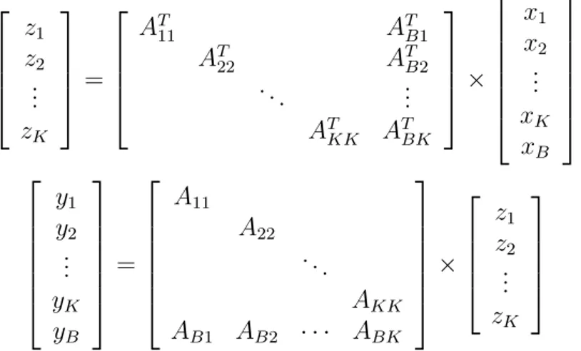
task-to-thread assignment scheme constitutes the CRp method as shown in Algorithm 1. Both in this algorithm and Algorithm 2, the “for . . . in parallel do” constructs shows each iteration of the for loop may be run in parallel. The matrix view of

the parallel CRp method given in Algorithm 1 is shown in Figure 4.1. xB and yB

vectors shown in this figure are also referred as “border subvectors” throughout the thesis.

It is well known that row-parallel and column-parallel SpMV algorithms re-spectively incur input and output dependencies among threads. As seen in Al-gorithm 1, the proposed method utilizing the SB form enables both input and output independent SpMV computations on diagonal blocks and their transposes

among threads. That is, SpMV computations zk ← ATkk xk and yk ← Akk zk in

lines 2 and 4 are performed concurrently and independently by threads. Note that the write-read dependency occurs between these two SpMV computations are in

fact intra-thread dependency due to the zk vector. Input dependency among

threads occurs in the zk ← zk + ATBk xB computation in line 3 via border

sub-vector xB. Output dependency among threads occurs in the yB ← yB+ ABk zk

computation in line 5 via border subvector yB.

As described above, partitioning and task-to-thread assignment used in the CRp method ensures that data which required in multiplication of every for-loop iteration fits into the cache of a single core. Therefore, both quality criteria (a) and (b) are satisfied by the CRp method through the reuse of z-vector entries and

     z1 z2 .. . zK      =      AT₁₁ AT_B1 AT 22 ATB2 . .. .._. AT KK ATBK      ×        x1 x2 .. . xK xB               y1 y2 .. . yK yB        =        A11 A22 . .. AKK AB1 AB2 · · · ABK        ×      z1 z2 .. . zK     

Figure 4.1: The matrix view of the parallel CRp method given in Algorithm 1. Algorithm 1 The proposed CRp method

Require: Akk and ABk matrices; x, y, and z vectors

1: for k ← 1 to K in parallel do 2: zk ← ATkk xk 3: zk ← zk+ ATBk xB 4: yk← Akk zk 5: yB ← yB+ ABk zk B Atomic 6: end for zk ← CkT x y ← Ck zk

That is, in y ← A z computation, no cache misses will occur neither in reading z-vector entries nor in accessing A-matrix nonzeros, under fully associative cache assumption. Note that only capacity misses and not conflict misses occur in a fully associative cache. In other words, under fully associative cache assumption, only compulsory misses due to writing z-vector entries and accessing A-matrix

nonzeros occur in zk ← CkT x and y ← Ck zk computations. Also note that in

order to satisfy the quality metric (b) A matrix must be stored only once, that

is, A and AT matrices cannot be stored separately. Specifically, nonzeros in the

diagonal blocks in zk ← ATkk xk and yk ← Akk zk computations are reused by

storing Akk in CSC format which corresponds to storing ATkk in CSR format or

vice versa. Similarly, nonzeros in the border blocks in zk ← zk + ATBk xB and

yB ← yB+ ABk zk computations are reused by storing ABk in CSC format which

corresponds to storing AT_Bk in CSR format or vice versa.

in accessing input-vector (x-vector) entries in row parallel SpMVs zk ← CkT x

through using the columnwise SB form of the AT _{matrix as follows: The diagonal}

block computations zk ← ATkk xk (line 2 of Algorithm 1) are independent in

terms of the x-vector entries thanks to columnwise SB form structure. Therefore, accessing x-vector entries will incur only one cache miss per entry, under fully

associative cache assumption. However, the border block computations zk ←

zk+ ATBk xB (line 3 of Algorithm 1) are dependent in terms of the x-vector entries

due to coupling columns in RT

B. Column cj having connectivity λ(cj) will result

at most λ(cj) misses due to accessing xj under fully associative cache assumption.

We should here mention that this upper bound on the number of cache misses

is rather a tight upper bound since such xj reuses can only occur when SpMV

computations associated with two border blocks that share nonzeros in column

cj are performed one after the other on the same core.

The CRp method satisfies quality criterion (d) by exploiting temporal locality

in updating output-vector (y-vector) entries in column parallel SpMVs y ← Ckzk

through using the rowwise SB form of the A matrix as follows: The diagonal block

computations yk← Akk zk(line 4 of Algorithm 1) are independent in terms of the

vector entries thanks to columnwise SB form structure. Therefore, accessing y-vector entries will incur only two cache misses (for reading and writing) per entry, under fully associative cache assumption. On the other hand, the border block

computations yB ← yB+ ABk zk (line 5 of Algorithm 1) do share y-vector entries

because of the coupling rows in RB. However, the border block computations

yB ← yB+ ABk zk (line 5 of Algorithm 1) are dependent in terms of the y-vector

entries due to the coupling rows in RB. Row ri having connectivity of λ(ri)

will result at most 2λ(ri) misses due to accessing yi under fully associative cache

assumption. Also, this upper bound on the number of cache misses is rather a

tight upper bound since such yi reuses can only occur when SpMV computations

associated with two border blocks that share nonzeros in row ri are performed

one after the other on the same core.

The CRp method satisfies quality criterion (e) by minimizing number of atomic updates on output-vector (y-vector) entries in column parallel SpMVs

diagonal block computations yk ← Akkzk (line 4 of Algorithm 1) are independent

in terms of yk-vector entries thanks to columnwise SB form structure .

There-fore, only one thread will be updating such yk-vector entries. However, the border

block computations yB ← yB+ ABk zk (line 5 of Algorithm 1) are dependent in

terms of yB-vector entries due to the coupling rows in RB. There are two possible

implementations of yB← yB+ ABk zk considering matrix storage scheme, namely

CSC and CSR. In the CSC scheme based implementation there will be one atomic

update operation for each nonzero of row border RB, whereas in the CSR scheme

based implementation there will be only one atomic operation for each nonzero

row of ABk matrices of RB. That is, to update yi ∈ yB, the CSC-based scheme

will incur one atomic operation for each nonzero in row ri, whereas CSR-based

scheme will incur λ(ri) atomic operations to update yi for row ri with a

connec-tivity of λ(ri). Therefore, the CSR scheme should be used in order to satisfy

quality criterion (e) since λ(ri) is much smaller then nnz(ri). So each border

block ABk is stored in CSR format, and hence correspondingly ATBk is stored in

CSC format.

As a result, minimizing the sum of the connectivities of coupling columns in

RT_B enables the proposed CRp method to satisfy criterion (c) and minimizing the

sum of the connectivities of coupling rows in RB enables to satisfy both quality

criteria (d) and (e). Note that columns of RT

B are identical to rows of RB,

there-fore the former and latter minimization objectives are equivalent. Consequently, permuting matrix A into rowwise SB form with the objective of minimizing the sum of the connectivities of coupling rows enables the CRp method to satisfy all of the three quality criteria (c), (d) and (e). Also note that, in that way inter-thread dependency is maximized, whereas intra-thread dependency is minimized.

A method for permuting sparse matrices into SB form via row/column reorder-ing is proposed by Aykanat et al. [32] usreorder-ing a hypergraph-partitionreorder-ing (HP). In this method the row-net hypergraph model [33] is used to permute matrix A into rowwise SB form as follows: Each column and row of matrix A correspond to a vertex and a net in the row-net model, respectively. The number of nonzeros in each column is assigned to corresponding vertex as weight. Unit cost assigned to nets. In a vertex partition of a given hypergraph, if a net contains at least one

vertex in a part, it connect that part. The number of parts connected by that net is referred with the connectivity of a net. If a nets connectivity is larger than one it is called as cut, and uncut otherwise. The HP problem constructed with the partitioning constraint, which is to balance the sum of weights of vertices in that part and with the partitioning objective, which is to minimize (cutsize) sum of the connectivities of the cut nets.

Matrix A is permuted into SB form ASBr by row/column reordering using a

K-way vertex partition of row-net model of matrix A as follows: The columns which are represented by the vertices of the k-th vertex part, correspond to the

column slice Ck, whereas uncut nets of the k-th part correspond to the set of

rows in row slice Rk of ASBr. The rows, which are represented by the cut nets,

constitute the row border RB of ASBr. The cut nets correspond to the rows of

the row border RB of ASBr. Also, the partitioning constraint correspond to the

balancing the number of nonzeros in the column slices. Note that this constraint also correspond to the load balancing between threads. Finally, the partitioning objective correspond to minimizing the sum of the connectivities of coupling rows

in the row border RB of ASBr.

On the other hand, the CRp method has a disadvantage. That is the z-vector is not finalized before the the y ← A z operation. Therefore, if an application requires an operation on z-vector, the CRp method is not applicable.

4.2

Row–Column-Parallel Method (RCp)

Consider a row/column reordering that permutes matrix A into rowwise SB form as: ˆ A = ASBc = PrAPc =        A11 A1B A22 A2B . .. .._. AKK AKB        =        R1 R2 .. . RK        = h C1 C2 . . . CK CB i . (4.5)

Rowwise SB form of AT _{could be induced from columnwise SB form of A as}

follows: (ASBc)T = ˆA = ATSBr = PcATPr=          AT₁₁ AT₂₂ . .. AT KK AT 1B AT2B ATKB          =          C₁T C₂T .. . CT K CT B          = h RT 1 RT2 . . . RTK i . (4.6)

In this method we partition rows and columns of matrix A and permutes matrix A into columnwise SB form, in such a way that the size of each column

slice Rk is equal to or less than the size of the cache of a single core. Algorithm 2

presents the RCp method. Also in the RCp method (as shown in Algorithm 2) both input and output independency among threads for SpMV computations on diagonal blocks and their transposes are enabled similarly to the CRp method

(as shown in lines 2 and 4). In a dual manner to CRp method, the zB ←

zB + ATkB xk computation in line 3 and the yk ← yk + AkB zB computation in

line 7 incur output and input dependency among threads via border subvector zB,

respectively. On contrast to the CRp method the RCp method requires additional synchronization overhead which is represented by the two consecutive “for . . . in

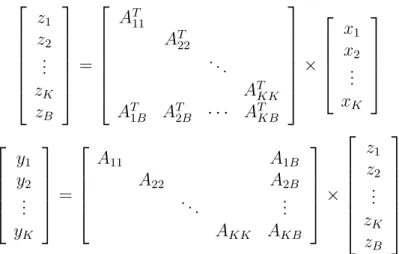
       z1 z2 .. . zK zB        =        AT 11 AT₂₂ . .. AT KK AT 1B AT2B · · · ATKB        ×      x1 x2 .. . xK           y1 y2 .. . yK      =      A11 A1B A22 A2B . .. .._. AKK AKB      ×        z1 z2 .. . zK zB       

Figure 4.2: The matrix view of the parallel RCp method given in Algorithm 2.

parallel do” constructs in Algorithm 2 due to the existence of both output and

input dependency on the same border subvector zB. The matrix view of the

parallel RCp method given in Algorithm 2 is shown in Figure 4.2. zB vector

shown in this figure is also referred as “border subvector” throughout the thesis. Algorithm 2 The proposed RCp method

Require: Akk and AkB matrices; x, y, and z vectors

1: for k ← 1 to K in parallel do 2: zk ← ATkk xk 3: zB ← zB+ ATkB xk B Atomic 4: yk← Akk zk 5: end for 6: for k ← 1 to K in parallel do 7: yk← yk+ AkB zB 8: end for z ← RT k xk yk← Rk z

The matrix partitioning scheme of the proposed RCp method can be consid-ered as dual of that of the CRp method given in Section 4.1. So the discussion about how the RCp method satisfies the quality criteria, in general, follows from the discussion in Section 4.1 on how the CRp method satisfies the quality cri-teria. Therefore, we just shortly summarize the discussion for the RCp method focusing on the differences. In general, all quality criteria are satisfied by the RCp method. Quality criteria (c)–(e) are satisfied for all respective

yk ← Akk zk computations. However, there are some deficiencies in the quality

criteria (a) and (b) due to zB ← zB+ATkB xkand yk← yk+AkBzB computations.

Although the RCp method has disadvantages as mentioned above, it can be still preferable because, rowwise partitioning might be more convenient for some of the nonsymmetric square and rectangular matrices, whereas columnwise partitioning might be more convenient for some other matrices. The fact that behind this difference is the row and column sparsity patterns as well as the dimensions of a given nonsymmetric or rectangular matrix. Hendrickson and Kolda [34] and U¸car and Aykanat [35] provide discussions on selecting rowwise or columnwise partitioning according to the matrix properties for the parallel SpMV operation.

Chapter 5

Experimental Results

The baseline method that we compare the performance of the proposed methods is given in Section 5.1. Hardware, software and parameters used in experimental setup are described in Section 5.2. Dataset and their properties that experi-ments are conducted on, are presented in Section 5.3. Finally, we report and discuss experimental results in Section 5.4 together with amortization values for the reordering overhead, scalability plots and matrix pictures.

5.1

Row–Row-Parallel Method (RRp)

In the RRp method given in Algorithm 3, both y ← A z and z ← AT _x

opera-tions are executed utilizing row-parallel SpMV. Therefore, the RRp method does

not require any atomic update operations. However, since A and AT matrices

are stored separately, exploiting temporal locality for the matrix nonzeros is not

possible between y ← A z and z ← AT _{x. In other words, quality criterion (b)}

(given in Chapter 4) is not satisfied. Also, quality criterion (a) is not completely satisfied, since the z-vector is generally quite large and would be evicted from cache before the y ← A z operation. Quality criterion (c) and (d) are not satis-fied without locality-aware partitioning. Finally, quality criterion (e) is perfectly satisfied, since there are no atomic updates.

The RRp method exists in the literature [23] and considered as state-of-the-art method. Therefore we used the RRp method as baseline method.

Algorithm 3 The baseline RRp method

Require: Matrix A of size M -by-N and its transpose AT_{; x, y, and z vectors,}

chunk size c 1: for k ← 1 to M/c in parallel do 2: zk ← ATkxk 3: end for 4: for k ← 1 to N/c in parallel do 5: yk← Akzk 6: end for

5.2

Experimental Setup

In our experiments, we use a machine that equipped with Intel Xeon CPU

E5-2643 running at 3.30 GHz and 256 GB of RAM as host system and single Intel R

Xeon PhiTM P5110 coprocessor as target system on which SpMV operations are

performed. The Intel R _{Xeon Phi}TM

supports both native and offload mode where the coprocessor runs standalone, and some code segments are offloaded to copro-cessor by host, respectively. We select offload mode. In the offload mode, 59 cores are available. Each core has 512KB Level 2 cache, and can execute up to four hardware threads.

In order to permute matrices into singly bordered block-diagonal (SB)

form, we use PaToH [36] which is hypergraph partitioning tool. We use

PATOH SUGPARAM SPEED since PaToH’s manual [36] states this parameter pro-duces reasonably good results much faster than PATOH SUGPARAM DEFAULT and PATOH SUGPARAM QUALITY provides only little better quality. The cuttype param-eter is set to connectivity-1 metric. Maximum allowed imbalance ratio between partitions is set to be 0.10. In order to find K, which is the number of parts, we compute size of matrix stored in CSR and CSC format in terms of kilobytes (KB) then divide by 64KB. Since four threads per core are running and cache

is not fully set associative we select partition size as 64KB. Since randomized algorithms are utilized in PaToH, we repeat each partitioning three times.

Sparse AATx Kernels are implemented in C using OpenMP and compiled with

ICC version 13.1.3 with flags openmp, parallel and O1. We used Ubuntu 12.04 as operating system.

We run Sparse AATx operation for 59, 118, 177, 236 threads which correspond

to 1, 2, 3, 4 hardware threads per core, respectively. We report best of them for each method. Dynamic scheduling and different chunksize (for baseline method 1, 2, 4, 8, 16, 32, 64, 128, 256, 512, 1024, 2048, 4096 and for proposed methods 1, 2, 4, 8, 16, 32) and best of them is reported. Environment variable for affinity is set as follows: MIC KMP AFFINITY=granularity=fine,balanced. For each method

and reordering, y ← AAT x computation run 1000 iterations after 10 iterations

as warm-up.

5.3

Dataset

We selected matrices according to applications discussed in Chapter 1, from the University of Florida Sparse Matrix Collection [37]. We present properties of these matrices in Table 5.1 sorted according to kind in alphabetical order. In the table, “Matrix” column shows the original name from the collection, and kind shows the application that the matrix is used. Web-link matrices, which are listed as kind of graph, are included since CG method can be used in the PageRank computations [11]. Also, average, maximum, standard deviation and coefficient of variation per row and column are given and labeled as “avg”, “max”, “std”, and “cov”, respectively. The coefficient of variation value for row or column should be considered as irregularity metric according to number of nonzeros.

Some matrices in the dataset could contain empty rows, columns or both. Since there is no multiplication with these rows or columns, they are removed and matrix is reordered accordingly. In the table, properties of such reordered matrices are given. Note that this reordering only effects the number of rows and

the number of columns. Also note that we included tall-and-skinny and short-and-fat matrices that the number of rows is much bigger than the number of columns and the number of rows is much smaller than the number of columns respectively.

T able 5.1: Prop erties of test matrices. Num b er of nnz’s in a ro w nnz’s in a col Matrix Kind ro ws cols nonzeros a vg max std co v a vg max std co v ASIC 680k circuit sim ulation problem 682,862 682,862 3,871,773 6 395,259 660 116 6 395,259 660 116 ASIC 680ks circuit sim ulation problem 682,712 682,712 2,329,176 3 210 4 1 3 210 4 1 circuit5M dc circuit sim ulation problem 3,523,317 3,523,317 19,194,193 5 27 2 0 5 25 1 0 F reescale1 circuit sim ulation problem 3,428,755 3,428,755 18,920,347 6 27 2 0 6 25 1 0 LargeRegFile circuit sim ulation problem 2,111,154 801,374 4,944,201 2 4 1 0 6 655,876 900 146 bib d 22 8 com binato rial problem 231 319,770 8,953,560 38,760 38,760 -28 28 -wheel 601 com binato rial problem 902,103 723,605 2,170,814 2 602 16 6 3 3 0 0 cnr-2000 directed graph 247,501 325,557 3,216,152 13 2,716 23 2 10 18,235 218 22 Stanford directed graph 261,588 281,731 2,312,497 9 38,606 173 20 8 255 11 1 Stanford Berk eley directed graph 615,384 678,711 7,583,376 12 83,448 300 24 11 249 16 1 w eb-BerkStan directed graph 680,486 617,094 7,600,595 11 249 16 1 12 84,208 300 24 w eb-Go ogle directed graph 739,454 714,545 5,105,039 7 456 7 1 7 6,326 43 6 w eb-Stanford directed graph 281,731 261,588 2,312,497 8 255 11 1 9 38,606 173 20 ESOC least squares problem 327,062 37,349 6,019,939 18 19 1 0 161 12,090 1,100 7 landmark least squares problem 71,952 2,673 1,151,232 16 16 -431 555 141 0 Maragal 7 least squares problem 46,845 26,525 1,200,537 26 9,559 288 11 45 584 34 1 sls least squares problem 1,748,122 62,729 6,804,304 4 4 1 0 108 1,685,394 6,852 63 con t1 l linear programming problem 1,918,399 1,921,596 7,031,999 4 5 1 0 4 1,279,998 923 252 dbic1 linear programming problem 43,200 226,317 1,081,843 25 1,453 41 2 5 38 4 1 dbir1 linear programming problem 18,804 45,775 1,077,025 57 3,376 220 4 24 223 35 1 degme linear programming problem 185,501 659,415 8,127,528 44 624,079 1,449 33 12 18 1 0 lp osa 60 linear programming problem 10,280 243,246 1,408,073 137 173,366 2,927 21 6 6 1 0 nemsemm1 linear programming problem 3,945 75,310 1,053,986 267 8,085 427 2 14 139 12 1 neos linear programming problem 479,119 515,905 1,526,794 3 29 1 0 3 16,220 46 16 rail2586 linear programming problem 2,586 923,269 8,011,362 3,098 72,554 6,506 2 9 12 2 0 stormG2 1000 linear programming problem 526,185 1,377,306 3,459,881 7 48 4 1 3 1,013 9 4 Eternit yI I E optimization problem 11,077 262,144 1,503,732 136 57,840 583 4 6 7 0 0 TSOPF RS b39 c30 p o w er net w or k problem 60,098 60,098 1,279,986 18 32 14 1 18 30,002 387 22 Cheb yshev4 structural problem 68,121 68,121 5,377,761 79 68,121 1,061 13 79 81 7 0 connectus undirected bipartite graph 458 394,707 1,127,525 2,462 120,065 7,979 3 3 73 4 2

5.4

Experimental Results

As mentioned above, we select and implement the RRp method as baseline. In

this method, we used the CSR-based implementation for both the A and AT

matrices. We conduct experiments with the RRp method on the original order, rowwise SB form and columnwise SB form. We run CSB method mentioned in

Chapter 3 on Intel R _{Xeon Phi}TM _{using micnativeloadex [38], however it did not}

scale on Intel R _{Xeon Phi}TM

. Therefore, we did not include results of the CSB [23] method here. Also the method proposed by Vuduc [30] is not reported, since it is much worse then the RRp method due to high number of atomic updates. Nonetheless, the CRp method with original order and the reordering given by HP is similar to Vuduc’s method.

In the CRp and RCp methods, as mentioned in Chapter 4, submatrices ABk

in the border are stored in CSR and CSC format, respectively. In the CRp

method, row border RB partitioned into ABk submatrices in CSR format, there

are many empty rows. That is additional for loop overhead is incurred due to these empty columns. Therefore, we use the generalized compressed sparse row (GCSR) format which has extra 1D array that stores indices for nonempty rows in irow array and main loop iterates on this array. The irow, icol, val arrays are the same as in the CSR format. The dual discussion holds for the RCp method,

so the generalized compressed sparse column (GCSC) format is used for ABk

submatrices. PaToH tries to place the rows that have similar sparsity pattern in the same block in rowwise partitioning, whereas it tries to place the columns that have similar sparsity pattern in the same block in columnwise partitioning. Therefore, cache locality is exploited better for vector entries when the CSC and CSR format in the CRp and RCp method, respectively.

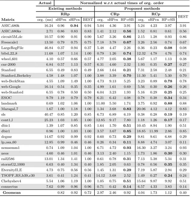
Performance comparison for the existing and proposed methods is given in

Ta-ble 5.2. In the taTa-ble, the second column shows actual run time of one Sparse AATx

operation for the RRp method with original order of the input matrix in terms of milliseconds. All other columns show normalized times with respect to the RRp method with unordered input matrix. The “org” stands for original ordering. In other words, we divided actual runtime of a given method by actual runtime of

the RRp method. Note that smaller value shows higher performance.

In the table, “sHPrn” and “sHPcn” stand for performance of the method that run on rowwise and columnwise partitioning utilizing HP, respectively. The CRp method is also run with the original order and sHPrn, whereas the RCp method is also run with the original order and sHPcn. These methods are not exactly same with the proposed Algorithm 1 and 2 but similar to the RRp method. The CRp method utilizes column-parallel SpMV for the y ← A z and row-parallel

SpMV for the z ← AT _{x, whereas the CRp method utilize row-parallel SpMV}

for the y ← A z and column-parallel SpMV for the z ← AT _{x. However, the SB}

form is not utilized in partitioning. In other words, these methods can be seen as

Algorithm 1 and 2 where the whole matrix is considered as border RB and CB,

respectively. The “HP-rSB” and “HP-cSB” columns stand for Algorithm 1 and 2, respectively.

In the table the best of the RRp method with original ordering and sHPrn and sHPcn is reported, as the best of the existing methods. Also the best of the CRp and RCp method is given. Note that best value for each matrix also is given in bold.

Table 5.2: Performance comparison of the proposed methods.

Actual Normalized w.r.t actual times of org. order Existing methods Proposed methods

RRp CRp RCp

BEST Matrix org. (ms) sHPrn sHPcn BEST org. sHPrn HP-rSB org. sHPcn HP-cSB ASIC 680k 16.24 0.96 0.94 0.94 5.04 4.36 3.91 5.24 4.23 3.97 3.91 ASIC 680ks 2.71 0.86 0.83 0.83 1.41 2.12 0.56 1.52 0.81 0.61 0.56 circuit5M dc 10.57 0.90 0.91 0.90 5.67 3.26 0.86 2.15 1.28 0.93 0.86 Freescale1 13.50 0.79 0.75 0.75 7.18 3.78 0.67 3.26 2.56 0.74 0.67 LargeRegFile 46.84 0.37 0.94 0.37 5.48 4.47 2.26 0.36 0.23 0.08 0.08 bibd 22 8 11.68 1.07 1.14 1.00 0.79 1.26 0.74 12.32 4.78 4.76 0.74 wheel 601 4.10 0.57 0.66 0.57 4.77 2.05 0.38 5.67 1.17 1.13 0.38 cnr-2000 6.84 0.57 1.13 0.57 6.31 4.60 2.32 1.93 0.35 0.27 0.27 Stanford 6.55 0.49 0.83 0.49 2.66 1.64 0.21 7.31 2.58 2.48 0.21 Stanford Berkeley 4.58 1.48 1.07 1.00 3.88 3.39 0.70 11.30 5.41 5.30 0.70 web-BerkStan 4.55 1.09 1.49 1.00 4.73 9.13 5.25 3.23 0.89 0.78 0.78 web-Google 16.14 0.54 0.35 0.35 4.99 1.61 0.69 5.56 0.30 0.26 0.26 web-Stanford 6.55 0.78 0.50 0.50 6.04 3.23 1.93 5.16 0.29 0.25 0.25 ESOC 9.79 1.19 0.79 0.79 6.21 6.42 4.08 0.78 0.38 0.34 0.34 landmark 0.69 1.02 1.06 1.00 11.00 5.50 1.74 3.75 0.92 0.88 0.88 Maragal 7 1.67 1.00 1.18 1.00 1.34 3.68 0.83 20.06 4.12 4.12 0.83 sls 40.47 0.85 1.20 0.85 6.73 6.89 6.19 0.38 0.28 0.19 0.19 cont1 l 25.23 1.03 1.05 1.00 12.85 9.17 7.80 1.18 1.26 0.17 0.17 dbic1 1.39 1.07 0.85 0.85 1.64 1.70 0.51 10.45 8.94 1.90 0.51 dbir1 0.96 1.00 1.03 1.00 3.57 3.67 0.85 18.85 11.99 2.86 0.85 degme 14.67 0.92 0.99 0.92 0.60 0.73 0.29 9.81 9.61 6.88 0.29 lp osa 60 12.85 0.99 0.46 0.46 0.26 0.34 0.11 8.88 4.74 3.07 0.11 nemsemm1 0.74 1.09 1.04 1.00 6.71 4.72 0.93 16.30 3.27 3.24 0.93 neos 4.60 0.46 1.01 0.46 3.13 2.40 1.15 1.73 1.86 0.30 0.30 rail2586 13.01 1.34 1.41 1.00 0.61 0.78 0.31 7.13 5.38 5.34 0.31 stormG2 1000 6.63 0.40 1.34 0.40 1.85 2.05 0.63 0.78 0.56 0.35 0.35 EternityII E 4.73 0.75 0.56 0.56 1.45 1.31 0.29 7.19 5.87 2.94 0.29 TSOPF RS b39 c30 3.61 0.41 1.24 0.41 14.12 3.68 2.52 1.49 0.27 0.24 0.24 Chebyshev4 5.54 1.06 1.19 1.00 1.05 0.75 0.51 15.64 9.87 9.92 0.51 connectus 7.62 0.99 0.96 0.96 0.71 0.42 0.14 6.57 4.33 3.83 0.14 Geomean 0.82 0.92 0.72 2.97 2.46 0.92 4.04 1.73 1.12 0.40

As seen in Table 5.2, on the average, the proposed methods either CRp or RCp outperforms baseline methods. Also, the RRp method with sHPcn and sHPrn orderings outperform the RRp method with original order since sHPcn and sHPrn exploit cache locality as discussed in [22]. As expected, the CRp method outperforms the RCp method, since the RCp method cannot satisfy all quality criteria. When best columns are compared, it is obvious that proposed methods are much better then the baseline method. In other words, proposed

methods reduce y ← AAT _{x time by 60% where the baseline method with sHPrn}

and sHPcn orderings can only reduce time by 28%.

Experimental results show that it is better to use the CRp method for short-and-fat matrices and the RCp method for tall-and-skinny matrices since number of atomic updates will be smaller and partitioning in larger dimension is better choice.

Note that for the CRp method comparison of the “org.” and “sHPrn”, and for the RCp method comparison of the “org.” and “sHPrn” show the importance of the exploiting cache locality for input and output vectors. As expected, in the CRp method, “sHPrn” outperforms “org.”, whereas in the RCp method “sHPcn” outperforms “org”.

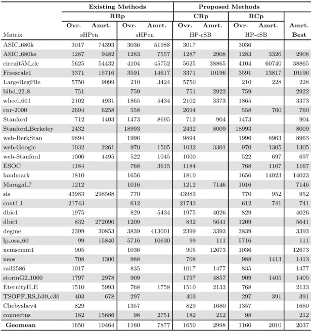
In Table 5.3, overhead and amortization values of the reordering methods are given. The columns labeled as “Ovr.” and “Amrt” correspond to overhead and amortization, respectively. The overhead value is normalized value of the

par-titioning time of PaToH with respect to one iteration of the y ← AAT _{x. The}

amortization value is the number of the y ← AAT _{x operations required to}

amor-tize the partitioning overhead. In the table, a blank cell corresponds to a negative value. In other words, when a method with ordering does not outperform than the RRp with original order, it cannot amortize the partitioning overhead. As seen in Table 5.3, on the average, as expected, overhead of the rowwise partition-ing and the columnwise partitionpartition-ing is comparable and the difference is due to the tall-and-skinny and short-and-fat matrices. Note that “Best” column gives combination of amortization values for the CRp and the RCp methods. Therefore

needed to amortize reordering overhead.

Table 5.3: Reordering overhead and amortization values.

Existing Methods Proposed Methods

RRp CRp RCp

Ovr. Amrt. Ovr. Amrt. Ovr. Amrt. Ovr. Amrt. Amrt.

Matrix sHPrn sHPcn HP-rSB HP-cSB Best ASIC 680k 3017 74393 3036 51988 3017 3036 ASIC 680ks 1287 9482 1283 7557 1287 2908 1283 3326 2908 circuit5M dc 5625 54432 4104 45752 5625 38865 4104 60740 38865 Freescale1 3371 15716 3591 14617 3371 10196 3591 13817 10196 LargeRegFile 5750 9099 210 3424 5750 210 228 228 bibd 22 8 751 759 751 2922 759 2922 wheel 601 2102 4931 1865 5434 2102 3373 1865 3373 cnr-2000 2694 6258 558 2694 558 760 760 Stanford 712 1403 1473 8695 712 904 1473 904 Stanford Berkeley 2432 18993 2432 8009 18993 8009 web-BerkStan 9894 1996 9894 1996 8963 8963 web-Google 1032 2261 970 1505 1032 3301 970 1305 1305 web-Stanford 1000 4495 522 1045 1000 522 697 697 ESOC 1184 768 3615 1184 768 1167 1167 landmark 1810 1656 1810 1656 14023 14023 Maragal 7 1212 1016 1212 7146 1016 7146 sls 43983 298568 770 43983 770 952 952 cont1 l 21743 612 21743 612 741 741 dbic1 1975 829 5434 1975 4026 829 4026 dbir1 832 272090 1209 832 5641 1209 5641 degme 2399 30853 3839 413001 2399 3393 3839 3393 lp osa 60 99 15840 5716 10630 99 111 5716 111 nemsemm1 905 1036 905 12673 1036 12673 neos 708 1300 988 708 988 1413 1413 rail2586 1017 835 1017 1477 835 1477 stormG2 1000 1797 2978 909 1797 4857 909 1405 1405 EternityII E 1510 5993 768 1758 1510 2133 768 2133 TSOPF RS b39 c30 403 678 297 403 297 391 391 Chebyshev4 829 1357 829 1680 1357 1680 connectus 182 15686 98 2751 182 212 98 212 Geomean 1650 10464 1160 7877 1650 2998 1160 2010 2037

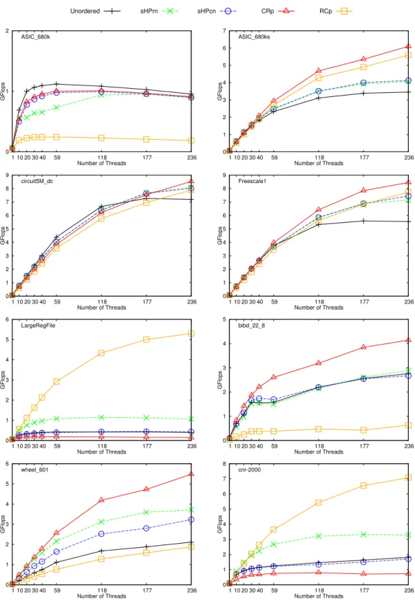
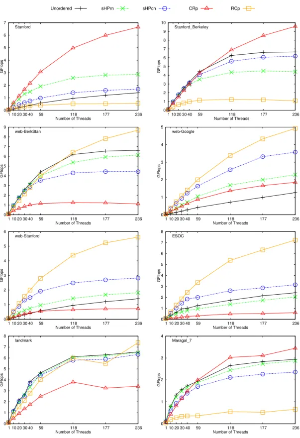
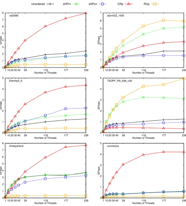
We also conduct scalability experiments with 1, 10, 20, 30, 40, 59, 118, 177, 236 threads. We present these results in Figures 5.1– 5.4. In these plots, y-axis represents performance in GFlops, x-axis represents number of threads and each curve represents a method. A legend for the methods is placed on the top per figure. In each plot, the corresponding matrix name is placed on top left corner. These plots show that our methods scale well as number of threads increase.

0 1 2 3 4 5 1 10 20 30 40 59 118 177 236 GFlops Number of Threads ASIC_680k Unordered sHPrn sHPcn CRp RCp 0 1 2 1 10 20 30 40 59 118 177 236 GFlops Number of Threads ASIC_680k 0 1 2 3 4 5 6 7 1 10 20 30 40 59 118 177 236 GFlops Number of Threads ASIC_680ks 0 1 2 3 4 5 6 7 8 9 1 10 20 30 40 59 118 177 236 GFlops Number of Threads circuit5M_dc 0 1 2 3 4 5 6 7 8 9 1 10 20 30 40 59 118 177 236 GFlops Number of Threads Freescale1 0 1 2 3 4 5 6 1 10 20 30 40 59 118 177 236 GFlops Number of Threads LargeRegFile 0 1 2 3 4 5 1 10 20 30 40 59 118 177 236 GFlops Number of Threads bibd_22_8 0 1 2 3 4 5 6 1 10 20 30 40 59 118 177 236 GFlops Number of Threads wheel_601 0 1 2 3 4 5 6 7 8 1 10 20 30 40 59 118 177 236 GFlops Number of Threads cnr-2000

0 1 2 3 4 5 1 10 20 30 40 59 118 177 236 GFlops Number of Threads ASIC_680k Unordered sHPrn sHPcn CRp RCp 0 1 2 3 4 5 6 7 1 10 20 30 40 59 118 177 236 GFlops Number of Threads Stanford 0 1 2 3 4 5 6 7 8 9 10 1 10 20 30 40 59 118 177 236 GFlops Number of Threads Stanford_Berkeley 0 1 2 3 4 5 6 7 8 9 1 10 20 30 40 59 118 177 236 GFlops Number of Threads web-BerkStan 0 1 2 3 4 5 1 10 20 30 40 59 118 177 236 GFlops Number of Threads web-Google 0 1 2 3 4 5 6 1 10 20 30 40 59 118 177 236 GFlops Number of Threads web-Stanford 0 1 2 3 4 5 6 7 8 1 10 20 30 40 59 118 177 236 GFlops Number of Threads ESOC 0 1 2 3 4 5 6 7 8 1 10 20 30 40 59 118 177 236 GFlops Number of Threads landmark 0 1 2 3 4 1 10 20 30 40 59 118 177 236 GFlops Number of Threads Maragal_7

0 1 2 3 4 5 1 10 20 30 40 59 118 177 236 GFlops Number of Threads ASIC_680k Unordered sHPrn sHPcn CRp RCp 0 1 2 3 4 1 10 20 30 40 59 118 177 236 GFlops Number of Threads sls 0 1 2 3 4 5 6 7 1 10 20 30 40 59 118 177 236 GFlops Number of Threads cont1_l 0 1 2 3 4 5 6 7 1 10 20 30 40 59 118 177 236 GFlops Number of Threads dbic1 0 1 2 3 4 5 6 1 10 20 30 40 59 118 177 236 GFlops Number of Threads dbir1 0 1 2 3 4 5 6 7 8 1 10 20 30 40 59 118 177 236 GFlops Number of Threads degme 0 1 2 3 4 5 1 10 20 30 40 59 118 177 236 GFlops Number of Threads lp_osa_60 0 1 2 3 4 5 6 7 1 10 20 30 40 59 118 177 236 GFlops Number of Threads nemsemm1 0 1 2 3 4 5 1 10 20 30 40 59 118 177 236 GFlops Number of Threads neos

0 1 2 3 4 5 1 10 20 30 40 59 118 177 236 GFlops Number of Threads ASIC_680k Unordered sHPrn sHPcn CRp RCp 0 1 2 3 4 5 6 7 8 1 10 20 30 40 59 118 177 236 GFlops Number of Threads rail2586 0 1 2 3 4 5 6 7 1 10 20 30 40 59 118 177 236 GFlops Number of Threads stormG2_1000 0 1 2 3 4 5 1 10 20 30 40 59 118 177 236 GFlops Number of Threads EternityII_E 0 1 2 3 4 5 1 10 20 30 40 59 118 177 236 GFlops Number of Threads TSOPF_RS_b39_c30 0 1 2 3 4 5 6 7 8 1 10 20 30 40 59 118 177 236 GFlops Number of Threads Chebyshev4 0 1 2 3 4 5 1 10 20 30 40 59 118 177 236 GFlops Number of Threads connectus

Pictures of A matrices in original order, rowwise SB form, columnwise SB form in subfigures (a),(b),(c), respectively given in Figures 5.5– 5.25. Note that pictures of the tall-and-skinny and the short-and-fat matrices are not given since they are not understandable.

These pictures show that either rowwise in CRp method or columnwise in RCp method partitioning does not produce high quality result, they cannot out-perform the RRp method due to the high number of atomic updates. For in-stance, both rowwise and columnwise partitioning could not achieved SB form for ASIC 680 k (see Figure 5.5) and the RRp method is performed better (see Ta-ble 5.2), although the original order is also irregular. If one of the rowwise and columnwise partitioning provides high quality SB form, as expected the CRp and RCp methods, respectively, achieve higher performance. As expected, if both rowwise and columnwise partitioning give good results, the CRp method outper-forms the RCp method since the RCp method partially satisfy quality criteria. Matrices Maragal 7 (see Figure 5.17) and degme (see Figure 5.21) show that the CRp method achieves higher performance than the RRp method, although the corresponding SB form is not very good, thanks to exploiting temporal locality for matrix nonzeros.

(a) Original Order (b) Rowwise SB (c) Columnwise SB

(a) Original Order (b) Rowwise SB (c) Columnwise SB Figure 5.6: Pictures of ASIC 680ks.

(a) Original Order (b) Rowwise SB (c) Columnwise SB

Figure 5.7: Pictures of circuit5M dc.

(a) Original Order (b) Rowwise SB (c) Columnwise SB

(a) Original Order (b) Rowwise SB (c) Columnwise SB Figure 5.9: Pictures of LargeRegFile.

(a) Original Order (b) Rowwise SB (c) Columnwise SB

(a) Original Order (b) Rowwise SB (c) Columnwise SB Figure 5.11: Pictures of cnr-2000.

(a) Original Order (b) Rowwise SB (c) Columnwise SB

Figure 5.12: Pictures of Stanford.

(a) Original Order (b) Rowwise SB (c) Columnwise SB

(a) Original Order (b) Rowwise SB (c) Columnwise SB Figure 5.14: Pictures of web-BerkStan.

(a) Original Order (b) Rowwise SB (c) Columnwise SB

Figure 5.15: Pictures of web-Google.

(a) Original Order (b) Rowwise SB (c) Columnwise SB

(a) Original Order (b) Rowwise SB (c) Columnwise SB Figure 5.17: Pictures of Maragal 7.

(a) Original Order (b) Rowwise SB (c) Columnwise SB

(a) Original Order (b) Rowwise SB (c) Columnwise SB Figure 5.19: Pictures of dbic1.

(a) Original Order (b) Rowwise SB (c) Columnwise SB

Figure 5.20: Pictures of dbir1.

(a) Original Order (b) Rowwise SB (c) Columnwise SB

Figure 5.21: Pictures of degme.

(a) Original Order (b) Rowwise SB (c) Columnwise SB

Figure 5.22: Pictures of neos.

(a) Original Order (b) Rowwise SB (c) Columnwise SB

(a) Original Order (b) Rowwise SB (c) Columnwise SB Figure 5.24: Pictures of TSOPF RS b39 c30.

(a) Original Order (b) Rowwise SB (c) Columnwise SB

Chapter 6

Conclusion and Future Work

In this chapter, we conclude our work in Section 6.1 and consider possible future work in Section 6.2.

6.1

Conclusion

In order to achieve high performance in Sparse AATx operations, temporal

local-ity for both matrix nonzeros and vector entries must be exploited. Also, minimiz-ing the number of atomic operations has a significant role in achievminimiz-ing high perfor-mance and scalability. It is possible to avoid atomic updates by storing the input matrix twice as in the RRp method, but exploiting temporal locality for matrix nonzeros would not be possible. In other words, there is a trade off between tem-poral locality of matrix nonzeros and atomic update operations. We proposed two parallel methods namely CRp and RCp for irregularly sparse matrix-vector and

matrix-transpose-vector multiply (Sparse AATx) operations that increase data

reuse. The CRp and RCp methods satisfy above requirements by utilizing singly bordered block-diagonal (SB) form enable reuse of matrix nonzeros and reduce the number of the atomic updates. We used rowwise and columnwise hyper-graph (HP) partitioning for reordering matrix into SB form for the CRp and RCp method, respectively.

We performed experiments with various kind of sparse matrices on Intel R

Xeon PhiTM. Experimental results showed that exploiting locality for vector

en-tries is not enough to attain high performance, also reusing the matrix nonzeros with minimum number of atomic updates is required. Therefore, our theory holds. As expected, the CRp method is generally better than the RCp method. On the other hand, sometimes the RCp method is better than the CRp method, since some of the matrices give higher quality result in columnwise partitioning due to their sparsity pattern and matrix dimensions. Consequently, proposed methods are better than state-of-the-art methods in the literature.

6.2

Future Work

We used CSR and CSC based SpMV in the inner kernel of methods, which are enough to show improvement of our methods. Moreover, other methods such as CSB and Vuduc’s algorithm could be integrated to our methods. Also, techniques like blocking or vectorization is possible. Integrating these might increase our performance gain in proposed methods.

The offload mode of the Intel R _{Xeon Phi}TM

enables hybrid parallelization by offloading different tasks to different coprocessors. It is possible to apply this technique in our methods.

Bibliography

[1] “Intel R _{Xeon Phi}TM _{Coprocessor - the Architecture.”}

https://software.intel.com/en-us/articles/

intel-xeon-phi-coprocessor-codename-knights-corner. Accessed:

2014-08-23.

[2] Y. Saad, Iterative Methods for Sparse Linear Systems. SIAM, 2003.

[3] W. Wang and D. P. O’leary, “Adaptive Use of Iterative Methods in Predictor–Corrector Interior Point Methods for Linear Programming,” Nu-merical Algorithms, vol. 25, no. 1-4, pp. 387–406, 2000.

[4] H. ¨Ozakta¸s, Algorithms for Linear and Convex Feasibility Problems: a

Brief Study of Iterative Projection, Localization and Subgradient Methods. PhD thesis, Bilkent University, Industrial Engineering Department, Ankara, Turkey, 1998.

[5] H. ¨Ozakta¸s, M. Akg¨ul, and M. C¸ . Pinar, “The Parallel Surrogate Constraint

Approach to the Linear Feasibility Problem,” in Applied Parallel Computing Industrial Computation and Optimization, pp. 565–574, Springer, 1996. [6] E. Turna, “Parallel Algorithms for the Solution of Large Sparse

Inequal-ity Systems on Distributed Memory Architectures,” Master’s thesis, Bilkent University, Computer Engineering Department, Ankara, Turkey, 1998. [7] K. Yang and K. G. Murty, “New Iterative Methods for Linear Inequalities,”

Journal of Optimization Theory and Applications, vol. 72, no. 1, pp. 163–185, 1992.

[8] B. U¸car and C. Aykanat, “Encapsulating Multiple Communication-Cost Metrics in Partitioning Sparse Rectangular Matrices for Parallel Matrix-Vector Multiplies,” SIAM Journal on Scientific Computing, vol. 25, no. 6, pp. 1837–1859, 2004.

[9] J. W. Demmel, Applied Numerical Linear Algebra. SIAM, 1997.

[10] J. M. Kleinberg, “Authoritative Sources in a Hyperlinked Environment,” Journal of the ACM (JACM), vol. 46, no. 5, pp. 604–632, 1999.

[11] G. M. D. Corso, A. Gull, and F. Romani, “Comparison of Krylov Subspace Methods on the PageRank Problem,” Journal of Computational and Applied Mathematics, vol. 210, no. 12, pp. 159 – 166, 2007.

[12] B. U¸car, C. Aykanat, M. C¸ . Pınar, and T. Malas, “Parallel Image Restoration

Using Surrogate Constraint Methods,” Journal of Parallel and Distributed Computing, vol. 67, no. 2, pp. 186–204, 2007.

[13] Y. Censor, Parallel Optimization: Theory, Algorithms, and Applications. Oxford University Press, 1997.

[14] G. H. Golub and C. F. van Van Loan, “Matrix Computations (Johns Hopkins Studies in Mathematical Sciences),” 1996.

[15] R. W. Freund and N. M. Nachtigal, “QMR: a Quasi-Minimal Resid-ual Method for Non-Hermitian Linear Systems,” Numerische Mathematik, vol. 60, no. 1, pp. 315–339, 1991.

[16] C. C. Paige and M. A. Saunders, “LSQR: An Algorithm for Sparse Linear Equations and Sparse Least Squares,” ACM Transactions on Mathematical Software (TOMS), vol. 8, no. 1, pp. 43–71, 1982.

[17] R. Fourer and S. Mehrotra, “Solving Symmetric Indefinite Systems in an Interior-Point Method for Linear Programming,” Mathematical Program-ming, vol. 62, no. 1-3, pp. 15–39, 1993.

[18] A. R. Oliveira and D. C. Sorensen, “A New Class of Preconditioners for Large-Scale Linear Systems from Interior Point Methods for Linear Pro-gramming,” Linear Algebra and Its Applications, vol. 394, pp. 1–24, 2005.

[19] Z. Bai, J. Demmel, J. Dongarra, A. Ruhe, and H. van der Vorst, Templates for the Solution of Algebraic Eigenvalue Problems: a Practical Guide, vol. 11. SIAM, 2000.

[20] A. Yzelman and R. H. Bisseling, “Cache-Oblivious Sparse Matrix-vector Multiplication by Using Sparse Matrix Partitioning Methods,” SIAM Jour-nal on Scientific Computing, vol. 31, no. 4, pp. 3128–3154, 2009.

[21] J. Koster, “Parallel Templates for Numerical Linear Algebra, a High-Performance Computation Library,” Master’s thesis, Utrecht University, De-partment of Mathematics, 2002.

[22] K. Akbudak, E. Kayaaslan, and C. Aykanat, “Hypergraph Partitioning Based Models and Methods for Exploiting Cache Locality in Sparse Matrix-Vector Multiplication,” SIAM Journal on Scientific Computing, vol. 35, no. 3, pp. C237–C262, 2013.

[23] A. Bulu¸c”, J. T. Fineman, M. Frigo, J. R. Gilbert, and C. E. Leiserson, “Parallel Sparse Matrix-Vector and Matrix-Transpose-Vector Multiplication Using Compressed Sparse Blocks,” in Proceedings of the twenty-first an-nual symposium on Parallelism in algorithms and architectures, pp. 233–244, ACM, 2009.

[24] A.-J. Yzelman and D. Roose, “High-level Strategies for Parallel Shared-Memory Sparse Matrix-Vector Multiplication,” IEEE Transactions on Par-allel and Distributed Systems, vol. 25, no. 1, pp. 116–125, 2014.

[25] M. Martone, “Efficient Multithreaded Untransposed, Transposed or Sym-metric Sparse Matrix-Vector Multiplication with the Recursive Sparse Blocks Format,” Parallel Computing, vol. 40, no. 7, pp. 251 – 270, 2014.

[26] A. Buluc, S. Williams, L. Oliker, and J. Demmel, “Reduced-Bandwidth Mul-tithreaded Algorithms for Sparse Matrix-Vector Multiplication,” in IEEE In-ternational Parallel & Distributed Processing Symposium (IPDPS), pp. 721– 733, IEEE, 2011.

[27] S. Williams, L. Oliker, R. Vuduc, J. Shalf, K. Yelick, and J. Demmel, “Op-timization of Sparse Matrix–Vector Multiplication on Emerging Multicore Platforms,” Parallel Computing, vol. 35, no. 3, pp. 178–194, 2009.

[28] N. Bell and M. Garland, “Efficient Sparse Matrix-Vector Multiplication on CUDA,” tech. rep., Nvidia Technical Report NVR-2008-004, Nvidia Corpo-ration, 2008.

[29] H. M. Aktulga, A. Bulu¸c, S. Williams, and C. Yang, “Optimizing Sparse Matrix-Multiple Vectors Multiplication for Nuclear Configuration Interac-tion CalculaInterac-tions,” Proceedings of the IPDPS. IEEE Computer Society, 2014. [30] R. W. Vuduc, Automatic Performance Tuning of Sparse Matrix Kernels.

PhD thesis, University of California, Berkeley, CA, USA, January 2004.

[31] E. Saule, K. Kaya, and ¨U. V. C¸ ataly¨urek, “Performance Evaluation of Sparse

Matrix Multiplication Kernels on Intel Xeon Phi,” in Parallel Processing and Applied Mathematics, pp. 559–570, Springer, 2014.

[32] C. Aykanat, A. Pinar, and mit V. Catalyurek, “Permuting Sparse Rect-angular Matrices into Block-Diagonal Form,” SIAM Journal on Scientific Computing, vol. 25, pp. 1860–1879, 2002.

[33] ¨U. V. Catalyurek and C. Aykanat, “Hypergraph-Partitioning-Based

Decom-position for Parallel Sparse-Matrix Vector Multiplication,” IEEE Transac-tions on Parallel and Distributed Systems, vol. 10, no. 7, pp. 673–693, 1999. [34] B. Hendrickson and T. G. Kolda, “Partitioning Rectangular and Structurally Unsymmetric Sparse Matrices for Parallel Processing,” SIAM Journal on Scientific Computing, vol. 21, no. 6, pp. 2048–2072, 2000.

[35] B. U¸car and C. Aykanat, “Partitioning Sparse Matrices for Parallel Precon-ditioned Iterative Methods,” SIAM Journal on Scientific Computing, vol. 29, no. 4, pp. 1683–1709, 2007.

[36] ¨U. V. Cataly¨urek and C. Aykanat, “PaToH: a Multilevel Hypergraph

Par-titioning Tool, version 3.0,” Bilkent University, Department of Computer Engineering, Ankara, vol. 6533, 1999.