Five essays on monetary policy applications in an open economy under economic uncertainty and shocks
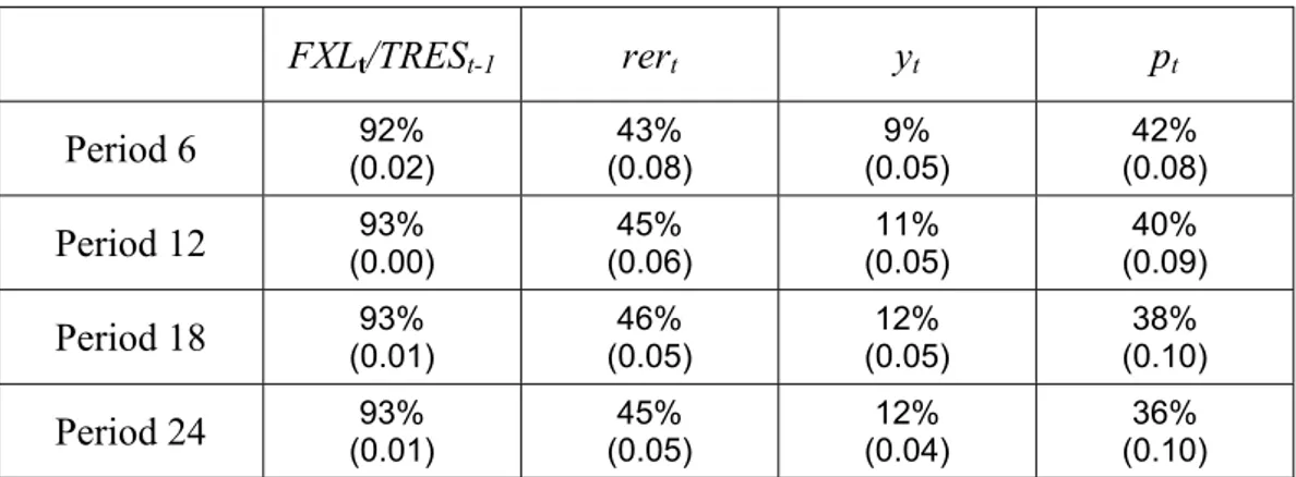
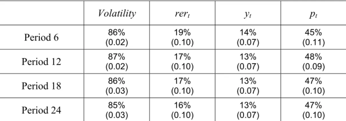
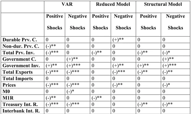
Tam metin
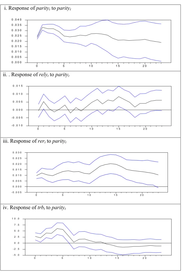
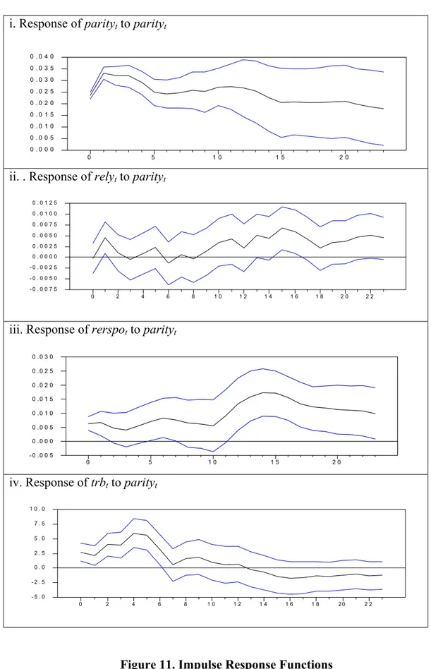
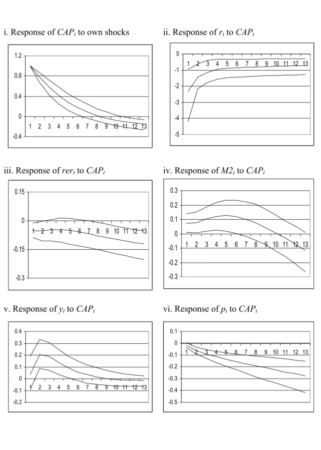
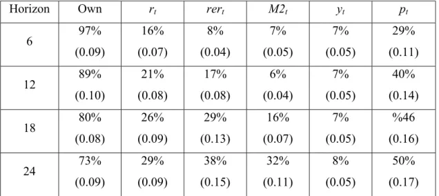
Şekil

Benzer Belgeler
During the compilation of Pascal source code, if Pascal compiler gener ates some errors resulting from the user’s incorrect flowchart design or syntax of the text
Pictorial Oculomotor Binocular Motional Occlusion Accommodation Binocular disparity Motion parallax Cast shadow Convergence Motion perspective Linear perspective Kinetic depth
Kamusal dış mekânlar için Kadıköy’deki yaşlıların 23’ü Landstraße’de ise 27’si güvenlik konusunda olumlu yorum yapmıştır (Resim 20).. Genel olarak
“Berâ-yı Sulhiyye-i Vehbî Efendi der-zamân-ı sadrâzâm İbrâhim Paşa” Seyyid Vehbî’nin (1674?-1736) Pasarofça (1718) üzerine, Sadrazâm Damat İbrahim Paşa’nın
Alkan gibi, onun daha c;ok birey merkezli bir tur liberalizmi savundugunu dil§iln- mekteler.7 Bu baglamda, Hilmi Ziya Ul- ken'in Tilrkiye'de (:agda§ Dil§ilnce Tari- hi adh
Initial results showed that polycrystalline wurtzite GaN thin films with low impurity contents can be deposited when the plasma-related oxygen contamination is
In this study, sediment loss due to sheet erosion occurring on the forest road slopes was investigated and the use of wood chips and slash to reduce soil loss was compared1. As a
Bu sayede gebelikte ağız bakımı konusunda gebelerin bilgi düzeyi arttırılabilir ve diş ve diş eti hastalıkları nedeniyle meydana gelen komplikasyonlar
