Adaptive filtering approaches for non-Gaussian stable processes

(1)

ADAPTIVE FILTERING APPROACHES

FOR NON-GAUSSIAN STABLE

PROCESSES

Orhan Arzkanl,

Murat

Belgel,

A .

Enis Cetin2 and Engin Erzin'

'Bilkent

University, Ankara, TURKEY.

2 K o ~

University, Istanbul, TURKEY.

ABSTRACT

A large class of physical phenomenon observed in practice exhibit non-Gaussian behavior. In this paper, a-stable distributions, which have heavier tails t h a n Gaussian distribution. are considered t o model non-Gaussian signals. A d a p tive signal processing in t he presence of such kind of noise is a requirement of many practical problems. Since, direct application of commonly used adaptation techniques fail in these applications, new approaches for adaptive filtering for a-stable random processes are introduced.

1. INTRODUCTION

In many signal processing applications t he noise is modeled as a Gaussian process. Thi s assumption has been broadly accepted because of t he Central Limit Theorem. However, a large class of physical observations exhibit non-Gaussian behavior, such as low frequency atmospheric noise, many types of man-made noise and underwater acoustic noise [1]- 131. There exists an important class of distributions known as a-stable distributions [ 5 ] which can be used t o model this type of noises. These distributions have heavier tails than those of Gaussian distribution, and they exhibit sh arp spikes or occasional bursts in their realizations. A random variable is called a-stable if its characteristic function has the following form:

o ( t ) = ezp{zat - yltl"[I

+

z p s z g n ( t ) w ( t , a ) ] } (1)

y

>

0 , 0

<

(Y

5

2, -1

5

,8

5 1

and

where --x,

<

a

<

CO,

t a n ( a a / 2 ) for a

#

1

a

log It1 for a = 1.

u ( t , a ) =

There is no compact expression for t he probability density function of these random variables except a = 1 and 2 cases which correspond t o the Cauchy and Gaussian distributions. respectively.

Llembers of stable distributions also satisfy a general- ized central limit theorem which states t hat if the s u m of i i.d. random variables converges then the limit distribution is a stable one. If individual distributions are of finite variance then t he limit distribution is Gaussian. Tails of this type of distributions are characterized with the a parameter ( 0

<

cy

5

2 ) which is called as t h e characteristic exponent ( N values close t o 0 indicates impulsive nature and a val-

u c s close to 2 indicates a more Gaussian type of behavior).

W i t h t h e Gaussian assumption, signals could be treated in

a Hilbert space framework which would allow t h e use of Lz (or

P;)

I.--= in various ont,imization criteria. Whereas. the linear vector space generated by a-stable distributions is a Banach space when (1

5

cy

<

2). In t h e linear space of

stable processes only p-norms exists for p

5

cy, hence.

norm cannot b e used with a n a-stable processes. Modeling a-stable processes under a Gaussian assumption leads t o unacceptable results as is reported in [5].

In this paper, various approaches t o adaptive filtering is investigated under additive a-stable noise with finite mean corresponding t o case of 1

5

a

<

2. These approaches are also compared t o recently introduced p-norm algorithms [4, 51. T h e p-norm algorithms are presented in Section 2 an d t h e use of pre-nonlinearity in adaptive filtering is investigated i n Section 3. T h e simulation results are given in Section 4.

2. ADAPTIVE FILTERING FOR a-STABLE

PROCESSES

T h e objective for a general filtering application is t o find an

FIR

filter of length

N ,

tu,t h a t relates t h e i n p u t , z ( n ) to

t h e desired signal d ( n ) :

@) =

&(k)'

(3 )

where d ( k ) is t h e estimate of t h e desired signal a t time instant

k,

a n d

-

z(k) = [z(k) z(k - 1) ' . . z ( k - N

+

l)]' . _{( 4 )} Commonly used adaptive filtering algorithms utilize the Hilbert space framework. This allows t h e use of least squares cost function whose solution can be found either exactly as

in Recursive Least Squares (RLS) algorithms or approxi- mated by Least-Mean-Squares (LMS) type methods [7, 81.

However, in t h e existence of a-stable processes least squares cost function cannot be defined because the variance of the error is not finite. Hence a new cost function other than least squares should be used.

I n this work, we consider a n adaptation algorithm for an F I R filter of length

N.

T h e problem is t o adaptively u p d a t e t h e tap weights of t h e FIR filter, zu, such t h a t given an input sequence ~ ( n ) , t h e output of t h e filter is close t o t he desired response d ( n ) , both of which is assumed t o be a-stable. In

this case, i t is appropriate t o minimize t h e dispersion of the error function [5].

(2)

This adaptation problem can be solved asymptotically by using the stochastic gradient method with the motivation of the LMS algorithm [8]. Such an algorithm, least mean p-norm ( L M P ) algorithm, is proposed in [ 5 ] . This algorithm is a generalization of instantaneous gradient de- scent algorithm t o a-stable processes, where the gradient of the p-norm of the error,

J = E[l4k)lPJ

= E[ld(k) - w(k)' E(k)lPl, 0

<

P

<

a ( 5 )

is used, and the t a p weights,

E,

are adapted at time step

k

+

1 as follows:

-

w ( k

+

1) =

d k )

+

I.L le(k)lP-' s g n ( e ( k ) )

c(k)

(6) where j~ is the step size which should be appropriately de-

termined. Note t h a t , for p = a = 2 the L M P algorithm reduces t o the well-known LMS algorithm [8]. When p is chosen as 1, the LMP algorithm is called the Least Mean Absolute Deviation (LMAD) algorithm 151:

-

w ( k

+

1) =

w(k)

+

I.L s g n ( e ( k ) )

c(k)

(7) which is also known as the signed-LMS algorithm.

In this paper we introduce two normalized adaptation algorithms with the motivation of the Normalized-LMS algorithm. T h e first one, Normalized Least Mean p-Norm (NLMP) algorithm, uses the following update:

where

P,A

>

0 are appropriately chosen update parame-

ters. In (8) normalization is obtained by dividing the update term by the p n o r m of the input vector,

~ ( k ) .

T h e reg- ularization parameter, A, is used t o avoid excessively large updates in case of a n occasionally small inputs. For p = 2, NLMP (8) reduces t o the Normalized-LMS algorithm [8].

T h e second algorithm, Normalized Least Mean Abso-

lute Deviation (NLMAD), corresponds t o t h e case of p = 1 in (8) with t h e following time update:

This adaptation scheme is especially useful when the char- acteristic exponent, a, either is unknown or varying in time. Among the stable distributions the heaviest tail occur for

the Cauchy distribution, a = 1. By selecting p = 1 the update term is guaranteed t o have a finite magnitude for all 1

< a

5

2 . Due t o the above reasons NLMAD is a safe

choice for the adaptation.

Recently, another class of normalized LMS type algorithms are also reported in [9, lo]. These algorithms are different from ours and they are developed in different con- text for white Gaussian input and Laplacian noise.

3.

USE

OF PRENONLINEARITY IN

ADAPTIVE FILTERING

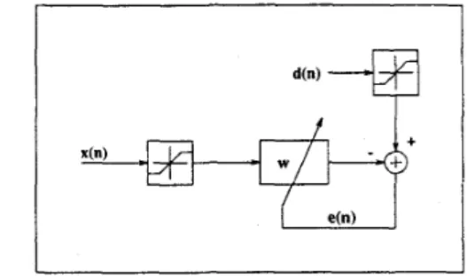
In this section t h e performance of LMS and RLS algorithms running on nonlinearly transformed d a t a will be investigated. In this paper, we consider the use of a softlimiter as

shown in Figure 1. T h e motivation behind this approach is able t o reduce the effect of spiky characteristic of the CY-

stable data.This type of regularization have been used in robust signal processing applications [ll]. I t can be easily shown t h a t any random process which is passed through a

softlimiter has finite variance. Thus, the LMS and RLS algorithms can be used in adaptation process after the input and reference signals have been soft-limited. T h e optimal filter coefficients which LMS and RLS converge are biased. However, the bias so introduced can be kept a t a reason- ably small level by a proper selection of threshold value. T h e use of softlimiter reduces the spiky characteristics of input d a t a hence a much smoother convergence can be ex- pected. Because of the use of a nonlinear mapping we call the well-known LMS and RLS algorithms as NMLMS and NMRLS. One noteworthy feature of this technique is that i t has the same computational complexity as well-known LMS and RLS algorithms. Because of the nonlinear mapping involved we call the proposed algorithms as

NMLMS

and NMRLS. A sample sequence of AR process disturbed by a-stable ( a = 1.8) noise and t h e output sequence after the soft limiter are shown in Figure 2.

Figure 1: Transform domain adaptive filtering block dia-

gram.

150, , , .

.

. ,

.

,

.

,

Figure 2 : A sample A R process disturbed by a-stable ( a = 1.8) noise ( a ) , and the output process after the soft limiter (b).

(3)

4. SIMULATION STUDIES

- 0 2 -

In simulation studies we consider A R ( N ) a-stable processes, which are defined as follows,

N

.(n) = a , z ( n - 2 )

+

a ( n ) (10)

t = l

where U(.) is a a-stable sequence of i.i.d random variables. The common distribution of ~ ( n ) is chosen t o be an even function

( p

= O ) , and the gain factors are all set t o one

( y = 1) without loss of generality. It can be shown t h a t z ( n )

will also be a a-stable random variable with t h e same characteristic exponent when { a , } is an absolutely summable sequence [5, 61.

T w o sets of simulation studies are performed. In the first set, the adaptation algorithms NLMAD, NLMP, LMAD, LhW and LMS are compared for a second order a-stable

A R

process with a fixed characteristic exponent, a = 1.2. In t h e second set the performances of NLMAD, NLMP, NMLMS and NMRLS algorithms are compared for a second order a-stable AR process with different values of the characteristic exponent. For both sets, the t a p weights are obtained by averaging 40 independent trials of the experiment and for each trial, a different computer realization of t h e process

{ U ( % ) } is used. To get a fair comparison between algorithms

the step sizes of adaptive algorithms are chosen in such a way t h a t they

aU

had a comparable steady-state variance. For both simulation set the coefficients of AR(2) is chosen as a1 = 0.99 and a2 = -0.1.

~ NLMAD - - - - LMAD

NLMP - - - LMp ... LMS

" f

l /

I

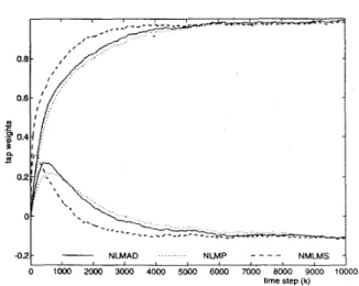
Figure 3: Transient behavior of tap weights in the NLMAD,

N L M P , L M A D , L M P and L M S algorithms with a = 1.2. In the first part of t h e simulations, A R parameters g

are estimated by a Z n d order LMP, LMAD, NLMP, NL- M A D and LMS algorithms. T h e plot of the t a p weights is given in Figure 3. In the first part we observed t h a t the

normalized algorithms NLMAD and NLMP outperformed other algorithms. Therefore, in the second part the performances of NMLMS and NMRLS are only compared to

NLMAD and NLMP algorithms.

In t h e second part of the simulations, A R parameters are estimated by a

and

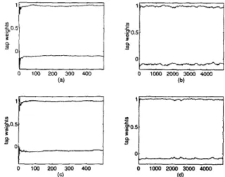
order NLMP, NLMAD, NMLMS and NMRLS algorithms for two different a-stable AR processes with a = 1.2 and a = 1.8. T h e plots of the t a p weights

for NLMAD, NLMP and NMLMS algorithms are given in Figure 4 and Figure 5 for a = 1.2 and a = 1.8, respectively. T h e t a p weights convergence performance of the NMRLS is given in Figure 6 for a = 1.2 and a = 1.8.

a2L - NLMAD NLMP - - - - NMLMS

4

1 I

0 1000 2000 3000 4000 5000 6000 7000 8000 9000 10000

nme step (k)

Figure 4: Transient behavior of tap weights in the

N M L M S ,

NLMAD, N L M P algorithms with a = 1.2.

0 2 - NLMAD NLMP - - - - NMLMS

0 < W O Moo 3000 4000 5000 6000 7oW 8000 9000 1

time step (k)

100

Figure 5: Transient behavior of tap weights in the N M L M S ,

NLMAD,

N L M P

algorithms with a = 1.8.

5. CONCLUSION

In this paper, new adaptive filtering approaches in t h e presence of a-stable random processes are introduced. These approaches are developed with t h e motivation of p-norm normalization in l p spaces 1

5

p

5

2, and the use of pre- nonlinearity in adaptive filtering. In our simulation studies the normalized algorithms NLMAD and N LM P outperform

(4)

the

LMAD, LMP

and LMS type algorithms. T h e use of pre- nonlinearity in

LMS

type algorithm exhibits a faster convergence than NLMAD and

NLMP

algorithms in the t a p weight adaptations. However, pre-nonlinearity introduced an off-set to the steady state values of the t a p weights. In our simulation examples, these off-set values are negli- gible, but it should be observed for higher order n-stable processes. T h e convergence of the RLS algorithm with the pre-nonlinearity outperforms other algorithms with a higher steady state variance. Also, NMRLS algorithm introduces an off-set, especially for low a values. T h e use of other non- linearities and the effect of off-set for higher order systems will be investigated as a future work.

’

7

O0 100 200 300 400 H .$0.5

e l

* I I 0 1000 2000 3000 4000 (b) O0 io00 2000 3000 4ooo M

Figure 6: Transient behavior of tap weights in the N M R L S

algorithm with a

=

1.8 (a,),@,), and a

=

1.2 (c),(d).

6. REFERENCES

B. blandelbrot and J .

Vf.

Van Ness, “Fractional brow- nian motions, fractional noises, and applications,” SIAM Review, vol. 10, pp. 422-437, 1968.

S.S. Pillai, M. Harisankar, “Simulated performance of a DS spread spectrum system in impulsive atmospheric noise,”

IEEE

Trans. Electromagnetic Compat., vol. 29, pp. 80-82, 1987.

M.

Bouvet and S. C. Schwartz,“ Comparison of adaptive and robust receivers for signal detection in am- bient underwater noise,”

IEEE

Trans. Acoust. Speech an d Signal Proc,, vol. 37, pp. 621-626, 1989.

0. Arikan, A.E. Getin and E. Erzin, “Adaptive filtering for non-Gaussian stable processes,” presented in Twenty-eight Annual Conference on Information Sci- ences a n d Systems, Princeton, N.J., March 1994. M. Shao and C. L. Nikiw, “Signal Processing with fractional lower order moments: Stable Processes and their applications,” Proc. IEEE, vol. 81, pp. 986-1009, 1993.

[6]

Y.

Hosoya, “Discrete-time stable processes and their certain properties,” Ann. Prob., vol. 6, no. 1, pp. 94-

105, 1978.

[ 7 ] J.

M.

Cioffi, “An Unwindowed RLS Adaptive Lattice

Algorithm,” IEEE Trans. on ASSP, vol. 36, no. 3 , pp. 365-371, March 1988.

[8] B. Widrow and S.D. Steams, Adaptive Signal Process- ing, Prentice Hall, NJ, 1985.

[9]

N.L.

Freire and S.C. Douglas, “Adaptive cancellation of geomagnetic background noise using a sign-error normalized LMS algorithm,” Proc. IEEE Innternationcd Conf. on Acoustics, Speech, a n d Signul Processing, vol 3, pp. 523-526, April 1993.

i

[lo] S.C. Douglas, “A Family of Normalized LMS Algo- rithms,” Signal Processing Letters, vol. l , no. 3, pp. 49-51, March 1994.

[ll] S.A. Kassam and H.V. Poor, “Robust techniques for

signal processing: a survey,” Proc. of IEEE, vol. 7 3 .

pp. 433-481, March 1985.