Mechanical and optical optimization of a fiber-optic interferometric acoustic sensor

MECHANICAL AND OPTICAL

OPTIMIZATION OF A FIBER-OPTIC

INTERFEROMETRIC ACOUSTIC SENSOR

a thesis submitted to

the graduate school of engineering and science

of bilkent university

in partial fulfillment of the requirements for

the degree of

master of science

in

materials science and nanotechnology

By

Ay¸seg¨

ul Abdelal

August, 2015

MECHANICAL AND OPTICAL OPTIMIZATION OF A FIBER-OPTIC INTERFEROMETRIC ACOUSTIC SENSOR

By Ay¸seg¨ul Abdelal August, 2015

We certify that we have read this thesis and that in our opinion it is fully adequate, in scope and in quality, as a thesis for the degree of Master of Science.

Assist. Prof. Dr. Aykutlu Dana(Advisor)

Assist. Prof. Dr. Necmi Bı yıklı

Assoc. Prof. Dr. Alpan Bek

Approved for the Graduate School of Engineering and Science:

ABSTRACT

MECHANICAL AND OPTICAL OPTIMIZATION OF

A FIBER-OPTIC INTERFEROMETRIC ACOUSTIC

SENSOR

Ay¸seg¨ul Abdelal

M.S. in Materials Science and Nanotechnology Advisor: Assist. Prof. Dr. Aykutlu Dana

August, 2015

External cavity Fiber optic interferometric microphones have the potential to operate at the acustic impedance derived noise limit, with a noise floor close to 1uP a/√Hz. This can be achieved with careful optimization of both the mechanical and optical properties of such a sensor. We describe models for the acoustic-to-displacement and displacement-to-optical signal transduction in a Fabry-Perot (FP) type interferometric microphone. We present experimental results and finite element calculations to validate the models. Based on the models, requirements to achieve ultimate sensitivity and noise level in a FP microphone are discussed. Demonstration of a microphone with 30 dBA noise floor is presented using partially optimized membrane and interferometer.

Keywords: Fabry- Perot interferometer, MEMS, optical microphone,acoustic sensor.

¨

OZET

FABRY-PEROT ˙INTERFEROMETR˙IK AKUST˙IK

SENS ¨

OR ¨

UN MEKAN˙IK VE OPT˙IK

OPT˙IM˙IZASYONU

Ay¸seg¨ul Abdelal

Malzeme Bilimi ve Nanoteknoloji, Y¨uksek Lisans Tez Danı¸smanı: Do¸c. Dr. Aykutlu Dana

A˘gustos, 2015

Harici kaviteli Fabry-Perot interferometrik mikrofonları , taban g¨ur¨ult¨us¨un¨un 1uP a/√Hz oldu˘gu, akustik impedanstan ayrılmı¸s g¨ur¨ult¨u seviyelerinde i¸sleme kapasitesine sahiptir. Bu d¨u¸s¨uk g¨ur¨ult¨u seviyesi, sens¨or¨un dikkatli mekanik ve optik optimizasyonlar sonucu elde edilebilir. Bu ¸calı¸smada, Fabry-Perot (FP) tipi interferometrik sens¨or¨un akustikten yer de˘gi¸stirmeye ve yer de˘gi¸stirmeden optik sinyale d¨on¨u¸st¨urme modelleri tanımlanmı¸stır. Modellere dayanarak deneysel ve teorik sonu¸clar incelenmi¸stir. 30 dBa taban g¨ur¨ult¨us¨u olan mikro-fon membran ve interferometrenin kısmi optimizasyonuyla g¨orselle¸stirilmi¸stir.

Acknowledgement

I would like to express my sincere gratitude, first and foremost, to my su-pervisor, Assist. Prof. Dr. Aykutlu Dana for his outstanding support, en-couragement and guidance throughout my research. I would like to thank the committee members, Assoc. Prof. Dr. Alpan Bek and Assist. Prof. Dr. Necmi Bıyıklı for their generous guidance and review on this work.

I also would like to expand my thanks to my group members, especially Gamze Toruno˘glu and Ahmet S¨onmez for their substantial contribution and all UNAM family.

Contents

1 Introduction 1

2 Fiber-Optic Interferometric Sensors 4

2.1 Classification of Fiber-Optic Interferometers . . . 6

2.1.1 Mach-Zehnder Interferometer . . . 7

2.1.2 Michelson Interferometer . . . 8

2.1.3 Sagnac Interferometer . . . 9

2.1.4 Fabry- Perot Interferometer . . . 11

2.2 Diaphragm-Based Fabry-Perot Interferometric Acoustic Sensor . 16 2.2.1 Acoustic Wave and Pressure . . . 18

2.2.2 Hearing Treshold . . . 19

CONTENTS vii

3 Mechanical Optimization of Fiber-Optic Acoustic Sensor 22

3.1 Membrane Mechanics . . . 23

3.1.1 Membrane Deflection . . . 23

3.2 Mechanical Optimization of Membrane Properties and Funda-mental Noise Sources . . . 27

3.2.1 Flat Membrane and MUMPS . . . 30

4 Experimental Process 42 4.1 Fabrication of Flat Membrane . . . 42

4.1.1 Wafer Cleaning . . . 43

4.1.2 Diaphragm Layer Deposition . . . 43

4.1.3 Photolithography and DRIE . . . 44

4.2 Multi-User MEMS (MUMPS) . . . 47

4.2.1 Fabrication Process . . . 47

4.2.2 Post Process . . . 48

4.3 Results . . . 48

5 Optical Optimization of Fiber- Optic Interferometric Acoustic

CONTENTS viii

5.1 Experimental Design . . . 57

5.2 Characterization Methods and Measurements . . . 60

List of Figures

2.1 Schematic structure of Mach- Zehnder interferometer . . . 7

2.2 Schematic structure of Michelson interferometer . . . 8

2.3 Schematic structure of Sagnac interferometric sensor . . . 10

2.4 Schematic structure of an extrinsic and intrinsic type of Fabry-Perot interferometer . . . 12

2.5 Gaussian wave propagation in a diaphragm based Fabry-Perot cavity . . . 13

2.6 Schematic illustration of beam waist and Rayleigh range . . . . 14

2.7 Schematic structure of a diaphragm based interferometric sensor 17

2.8 Ratio of transmitted and incident light intensity as a function of phase difference[1] . . . 21

LIST OF FIGURES x

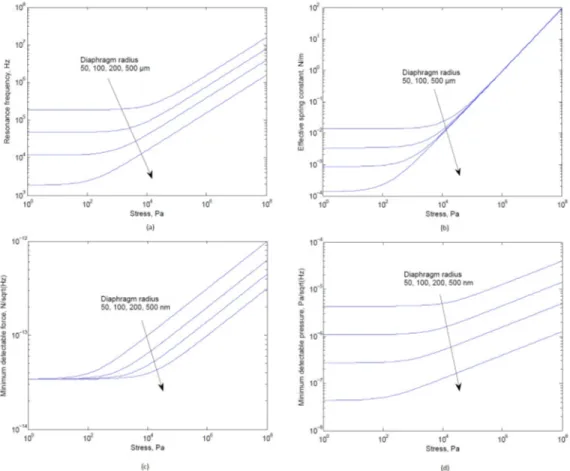
3.1 a) Resonance frequency b) effective spring constant c) minimum detectable force limited by Brownian motion and d) minimum detectable pressure values are shown as functions of stress and diaphragm radius for 50 nm thick Si3N4 diaphragm. Here, noise

of interferometer is defined as Shot noise level that is obtained by 500µW impulse power and 50 A/m interferometer sensitivity. Thermal limit, the minimum detectable pressure (600nP a/√Hz ) around 30 kHz), and threshold of hearing 20 µP a (d) are shown with red lines. . . 34

3.2 For 50 nm thick Si3N4diaphragm with 50, 100, 200, and 500 µm

radius a)Resonance frequency, b) Effective spring constant, c) minimum detectable force and d) pressure caused by Brownian noise are shown as functions of stress and radius of diaphragm. Here, noise of interferometer is defined as Shot noise level that is obtained by 500 µW is impulse power and 50 A/m interfer-ometer sensitivity. . . 35

3.3 Noise levels in terms of frequency are shown when Q=1 for 50 nm thick Si3N4 diaphragm with 500 µm radius. a) Brownian

motion noise dependent on frequency and b) The minimum de-tectable pressure at different stress values are shown for 500µW is impulse power and 50 A/m interferometer sensitivity. Red line indicates thermal limit which is 600 nP a/√Hz. . . 36

3.4 COMSOL simulation results compared with membrane deflec-tion model . . . 37

LIST OF FIGURES xi

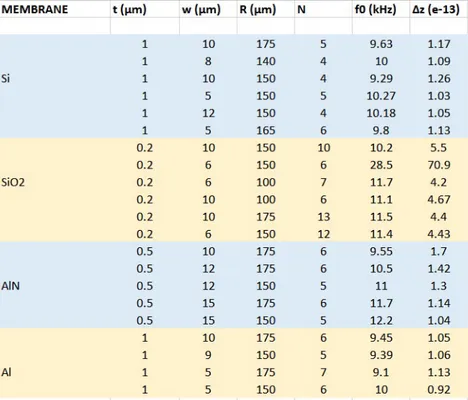
3.6 Geometrical parameters for Si, SiO2, Al and AlN membranes

and their calculated resonance frequency . . . 38

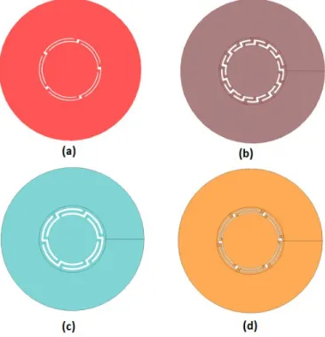
3.7 a)Si Membrane Din = 350 µm Dout = 750 µm t = 1 µm w =

10 µm N= 5, b) SiO2 Din = 350 µm Dout = 750 µm t = 0.2

µm w = 10 µm N= 13, c) AlN Din = 350 µm Dout = 750 µm t

= 0.5 µm w = 12 µm N= 6, d) Din = 350 µm Dout = 750 µm

t = 1 µm w = 10 µm N= 6 . . . 39

3.8 Finite element analysis of Si MUMPS membranes with specified geometrical parameters . . . 40

3.9 Finite element analysis of Si MUMPS membrane with specified geometrical parameters . . . 41

4.1 Fabrication process steps of Al2O3 diaphragm . . . 49

4.2 shows the schematic structure of diaphragm holder obtained by Si wafer etching. There are four sizes of holders those are 100 and 150 µm inner radius and 400 µm outer radius. The outer radius value is constant by the purpose of the diaphragm is planned to be clamped to the ferrule which has also 400 µm radius. Fig. (b) is the image of photo-mask design showing the four structures. . . 50

4.3 Microscope images Si wafer after development a) t=20 µm R1=150 µm b) t=30 µmR2= 100 µm . . . 50

LIST OF FIGURES xii

4.5 DRIE recipe before optimization . . . 51

4.6 Tilted and top view of Si membrane holders after 1h DRIE run 52

4.7 Effects of DRIE process parameters on etch rate, profile, selec-tivity, grass, breakdown and sidewall [36] . . . 52

4.8 Improved DRIE recipe . . . 52

4.9 Profile and tilted SEM images of Si membrane holders after 1 h run with improved recipe . . . 53

4.10 Profile and tilted SEM images of Si membrane holders after 2.5 run with improved recipe . . . 53

4.11 Fabrication steps of Piezo MUMPS process . . . 54

4.12 SEM images of 4 different types of MUMPS membranes . . . 55

4.13 SEM images of 3 different types of MUMPS membranes after etching . . . 56

5.1 a) Setup for experimental study of fiber optic interferometric microphone. b) Schematic demonstration of the same setup . . . 58

5.2 The image of the fiber interferometer for two different location. Distance between fiber and diaphragm can be set around 150 um manually . . . 59

LIST OF FIGURES xiii

5.3 a) Laser intensity noise is 500 µW impulse and for 1 µA/W gain . b) Relative intensity noise (RIN) level is around 0.2%. This value is 100 times higher than Shot noise level and needed to be removed by a stabilization circuit. . . 60

5.4 a) Ferrule and glass jacket that is going to hold the diaphragm b) Microscope image of 50 nm thick Silicon Nitride diaphragm. It became semi-transparent with 15 nm gold coating on both sides. . . 61

5.5 a) Background noise measured with fiber-optic microphone and b) Hello! . . . 62

5.6 a) Laser intensity noise is around 10 mV for for 500 µW impulse and 1 µA/V gain values. B) Relative intensity noise (RIN) is at 0.2% level. This value is 100 times greater than Shot noise and need to be reduced by a stabilization circuit . . . 63

5.7 Background noise level is 20 mV pp when measured by the ADMP401 test microphone. Considering the existing configura-tion 1 Pa pressure corresponds to 513 mV. Thereby, background noise is approximately 40 mPa pressure level. The background noise is regarded as degradable when fiber microphone is stabi-lized. . . 63

5.8 Response of ADMP401 to 1 kHz test signal. a) After test signal is over, background noise becomes dominant factor. . . 64

LIST OF FIGURES xiv

5.9 Response of interferometric microphone to 3 kHz test signal. After test signal is over, background noise becomes dominant factor. Here, 500 µW laser power and 150 µm interferometer gap are used. . . 65

5.10 Frequency responses of ADMP401 and fiber-optic microphone were measured with frequency sweep. In the consequence of sound source was not ideal, unexpected responses was seen es-pecially for low frequencies. Nevertheless, it can be deduced that these two microphones are comparable and they consist the audible band. . . 66

5.11 a) Interferometric microphone and b) ADMP401 responses for sound signals. Compared to fiber-optic microphone ADMP401 has a couple of times larger signal noise ratio (SNR). . . 67

Chapter 1

Introduction

Fiber optic sensors have recieved remarkable interest due to their performance in the last few decades [2]. Development of fiber optic technology lead their investigation in sensing applications owing to the advangates. The unique char-acteristics including low propagating loss, low cost, high sensitivity, enabling device miniaturization, high detection bandwidth, environmental durableness, multiplexing, and remote sensing caused an increasing interest in fiber-optic technology [3]. The outstanding features and performance have being used for various measurands such as temperature, strain, pressure, displacement, rota-tion, current measurements, refractive index, roughness, and acceleration. Op-tical fibers have very small size, on the order of microns in diameter makes them lighter and smaller over their electronic competitors. In addition to these, the sensing yield can be promoted according to the measurand by counting in fiber gratings, interferometers, surface plasmon resonance (SPR), micro-structured fibers and so on [4-6].

be executed by modulation in intensity, phase, polarization or wavelength. The applications especially those are commercialized such as gyroscope and hydrophone, have been offering high reliability, sensitivity and low cost. These advantages of fiber-optic sensors have made them focalized to study on com-pared to their conventional counterparts, in a broad range of applications.

One of the most important application of fiber-optic sensors is acoustic sensors. First optical fiber interferomteric acoustic sensor was presented by Bucaro et al. [7,8]. They have used Mach- Zender sensor[add] for detecting sound waves underwater. Their focus was on single and multi-mode, low-loss optical fibers used for increasing the sensitivity of acoustic detection. A double fiber path interferometer system is employed where one fiber is exposed to the acoustic wave. Single mode fiber Fabry Perot configuration was also developed that is able to provide high sensitivity [4].

Engineering and research studies pay remarkable attention to acoustic sen-sor technology. Numerious applications of acoustic wave sensen-sors have been in use such as navigation, material characterization, and in medical diagnostics [10,11]. Furthermore, fiber-optic sensors are favorable to use in high electric-field environments because of they are passive to electromagnetic effects. In medical applications electrical isolation which is essential for patients can be provided by fiber-optic sensors which are also chemically and biologically inert. Apart from this, aearospace area is availed by the advantages of light weigh and small size of the fiber-optic devices. Considering the requirements such as heavy shielding, cost, size and weight that conventional electrical sensors have, fiber-optic sensors have great supremacy in terms of efficiency, cost size and durability that enables high temperature operation and high vibration re-sistance [5]. In this thesis we have focused on fiber-optic microphones which

Having a number of subsistent benefits, including small size, light weight, high sensitivity, high frequency response, and immunity to electromagnetic interference, optical fiber-based sensors have been proven to be attractive to measure a wide range of physical and chemical parameters. In summary, fiber-optic interferometric sensors has gained a high reputation regarding their abil-ity to have high sensitivabil-ity, various designs and low cost. Nonetheless, the interference has a nonlinear nature posing an obstacle while optimizing the fiberoptic interferometer [6]. Enhanced transduction is required to improve the sensitivity of the fiber-optic sensor which could increase the cost and the challenge.

Chapter 2

Fiber-Optic Interferometric

Sensors

For the measurements of displacement, temperature, strain, pressure and acoutic signals, fiber-optic interferometric sensors have drawn interest due to their advantages over conventional sensors. They also form a large and im-portant subgroup of intrinsic fiber-optic sensors due to their high performance [5].

An interferometer is an optical device that utilises the superposition of two beams propagating through different optical paths those are on single fiber or two fibers for the fiber-optic interferometers. One of the path should be sensitive to be effected by external influences like change of length of path or refractive index in order to create interference. To make them travel different optical paths beam splitters and combiners are used in desired configurations [7]. By virtue of the ability to detect external perturbations,the interferometer

as frequency, phase, bandwidth, intensity and wavelength. Furthermore, the information obtained from the sensor can be both time-dependent or spectral. In recent developments of fiber-optic interferometer, reducing the size of sensor is one of the most focused area to extend its application field and take the advantage of easy alignment, high coupling efficiency and high stability [8].

In this chapter fiber-optic interferometers and their types are briefly ex-plained in terms of their operating principle, application fields, advantages and challanges.

2.1

Classification of Fiber-Optic

Interferome-ters

Fiber-optic interferometers can be categorized into four types those are Michel-son, Mach Zender, Sagnac and Fabry- Perot Interferometer. They are also considered as great alternatives for acoustic wave detection. In the first years of fiber-optic sensor progress, Mach-Zender and Michelson which are intrin-sic types of interferometric sensors were considered for acoustic wave sensing [9]. Two main drawbacks have appeared related to the requirement of long fiber in order to increase sensitivity for these two types. This requirement results vulnerable to undesired temperature or vibration, and instability. In addition, polarization-fading issue caused by two beams interfere coincidental due to the change in the polarization of the travelling beam in the fiber [10]. Although for acoustic pressure sensing, Sagnac interferometer has advantages over Mach-Zender and Michelson interferometer in the case of phase noise is-sue, instability and phase-fading problem still exist in Sagnac interferometer sensor [6]. The last fiber-optic interferometric sensor that will be discussed is Fabry-Perot interferometer. Fabry-Perot interferometer has preeminence due to its smaller device size and stability which makes it the most suitable acous-tic wave sensor over other types of fiber-opacous-tic interferometers [11]. Besides optical fiber interferometers have great advantage in terms of sensitivity and variety of device designs, thorough optimization should be executed in order to gain higher performance.

2.1.1

Mach-Zehnder Interferometer

Mach-Zehnder Interferometer (MZI), has been developed for different kinds of sensor applications based on its advantages of alterable instrument design. Common MZI structure comprises two independent optical paths which are called reference and sensing arms. Figure 2.1 illustrates the basic schematic structure of MZI where the incident beam is separated into two parts by a beam splitter. They are assumed that beam is splitted in two equal powered laser beam. After these two beams are traversing through reference and sensing arms, they are recombined by a second coupler [6].

Figure 2.1: Schematic structure of Mach- Zehnder interferometer

Reference arm is shielded properly from environmental influences so as to sensing arm is the only optical path exposed to external perturbations such as acoustic field in our case. The superposition of the recombined beams creates a phase change caused by the optical path length difference between two propagating beams. The interference signal between two beams formed after propagating the length of the output fiber is detected by photodetectors. The phase shift can be associated by the acoustic pressure by analyzing the variation in the output signal. As mentioned before, MZI sensors first arised in 70s by Bucaro et. al. [12], requiring long fibers which are used for increasing the responsivity, making them bulky instruments. Other problems with MZI sensors include environmental effects such as temperature fluctuations and pressure changes, also cause signal degeneration and polarization fading [13]

[14].

2.1.2

Michelson Interferometer

Michelson interferometer (MI) is another implementation of classical fiber-optic interferometers similar to MZI in respect of having two separated arms, sensing and reference coils. However in this case, there is a single fiber coupler which both splits and recombines the light beams. The laser light coming out from the source is split into two beams travelling through reference and sensing arms. After traversing the length of the arms, the beams are reflected through the same arms by the reflectors end of the arms. Afterwards the beams are recombined by the beam splitter as shown in Figure 2.2, they are directed to the photo detector.

Figure 2.2: Schematic structure of Michelson interferometer

Since MI sensors are a folded version of MZI sensors, fabrication process, optical loss quantity and operating systems are also similar. The main differ-ences are reflectors end of the arms in MI and having only one fiber coupler in the configuration. Owing to the fact that the light passes through both sensing and reference arms twice, the optical phase shift per unit length is doubled [5]. Another benefit of MI sensors is having one less fiber coupler prevents extra 12-dB loss in signal. Although it seems MI sensors have more compact design

which more practical, the advantage depends on the application field. MI sen-sors have several advantages where multiplexing ability is among them. For MI sensors it is important to adjust the length difference of the fibers between the two arms while connecting multiple sensors in parallel. On the other hand in-line structure is another possibility for MI sensors. To form an in-line con-figuration, some part of the incident beam is coupled to cladding mode from core mode. Hence the beam uncoupled by the reflector can traverse until the end of the fiber [6].

Similarly for the Michaelson type of interferometric acoustic sensor, the initial light beam is split into two beams which are reference and test beams. Distinctly in Mach-Zehnder interferometric microphone, after an optical beam is split into a test and a reference beam using a beam splitter they are recom-bined by a second coupler in order to detect the phase shift while the length of the test beam changes during the membrane vibration. In Michaelson config-uration, there is only one fiber coupler that light pass through twice. Hence, while the beams traversing in reference and test arms, optical phase shift per unit length is twice larger compared with Mach- Zehnder interferometer. Prof-itably, Michaelson interferometric sensor can be shrinked in accordance with the reduced quantity of the components.

2.1.3

Sagnac Interferometer

Third interferometer reviewed in this chapter is Sagnac interferometer (SI). Dissimilarly to the previous two interferometers mentioned above, Sagnac in-terferometers solve some issues that those faced. In SI configuration, there is an optical fiber in a loop, and two light beams propagate along this fiber in

counter directions with different polarization states. SI can be defined as a fiber loop that employs a delay and a sensing coil which are located asymmetrically in the sensor configuration [6].

Figure 2.3: Schematic structure of Sagnac interferometric sensor

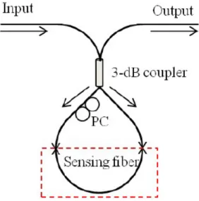
Light from the source is split into a clockwise (CW) and a counterclock-wise (CCW) signal by an optical coupler. The CW and CCW signals arrive at the sensing section at different times, during which the incident acoustic field changes. This results in a difference in the acoustically induced phase change experienced by the counter-propagating signals as they travel through the sensing coil. Unlike other fiber optic interferometers, the OPD is deter-mined by the polarization dependent propagating speed of the mode guided along the loop. To maximize the polarization-dependent feature of SIs, bire-fringent fibers are typically utilized in sensing parts. The polarizations are adjusted by a polarization controller (PC) attached at the beginning of the sensing fiber. The signal at the output port of the fiber coupler is governed by the interference between the beams polarized along the slow axis and the fast axis [6].

2.1.4

Fabry- Perot Interferometer

The interferometric sensor type that is focused on in this thesis is the Fabry-Perot interferometric sensor. A Fabry-Fabry-Perot (FP) interferometer consists of a resonant optical cavity including two reflectors located closely [15]. Fabry-Perot interferometer (FPI) was invented by Charles Fabry and Alfred Fabry-Perot in 1897 [16]. Distinct from the interferometers viewed before, FPI sensors involves multiple beam interference which provides sharper resonances at particular frequencies. Hence the sensitivity level is much higher than other types of interferometers.

A general configuration of a FPI consists of two reflecting plates which are separated at a fixed distance. This structure is also called as etalon [17]. Multiple beam interference takes place in FPI as mentioned above, which is formed by the reflected and transmitted beams from these two surfaces. To carry out FPI to fiber-optic applications, the etalon can be created by the fibers used. The reflectors required can be placed both inside or outside the fibers, which make it separated into two groups. One is extrinsic and the other one is intrinsic type of FPI. Figure 2.4 illustrates both types, (a) extrinsic and (b) intrinsic type, of FPI with schematic structures. The extrinsic type of FPI involves its cavity outside the related fiber. These kind of structure can provide high finesse interference and cheap equipment due to its simplicity.

Interference occurs due to the multiple super positions of both reflected and transmitted beams at two parallel surfaces. For the fiber optic cases, the FPI can be simply formed by intentionally building up reflectors inside or outside of fibers. FPI sensors can be largely classified into two categories: one is extrinsic and the other is intrinsic. The extrinsic FPI sensor uses the

Figure 2.4: Schematic structure of an extrinsic and intrinsic type of Fabry-Perot interferometer

reflections from an external cavity formed out of the interesting fiber. Figure (a) shows an extrinsic FPI sensor, in which the air cavity is formed by a supporting structure. Since it can utilize high reflecting mirrors, the extrinsic structure is useful to obtain a high finesse interference signal. Furthermore, the fabrication is relatively simple and does not need any high cost equipment.

One of the drawbacks that FPI may have is the alignment challenge of the cavity and accordingly the coupling efficiency [18]. There are also reflecting surfaces in the fiber itself which makes possible to have both internal and external interferences. The parallel surfaces have reflectivity constants R1 and

R2 forming the cavity, and located at a fixed distance, d apart. The optical

phase difference between the initial light beam and reflected beam cause the intensity modulation that forms the spectrum of FPI [19]. Multiple reflections and transmissions enhances the interference signal output. The optical path that light travels is proportional to the integer number of half wavelength of the initial light. Thus, the phase difference can be expressed as,

δ = 2kdn cosθ (2.1)

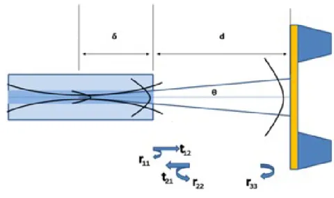
Where λ is the wavelength of incident light, n is the refractive index of cavity material or cavity mode, and L is the physical length of the cavity. θ represents the angle between the transmitted light and the surface normal of the reflecting surface. In FP interferometer, multi-beam interference in a cavity is used. Multiple beam interference occurs when a light beam on a transparent plate, there are multiple reflections at the surface of the plane with the result of a series of beams of diminishing amplitude emerges on each side of the plate [1]. The configuration we discuss involves the cavity formed by a diaphragm and the fiber tip. In our case, we take into account multiple reflections in FP cavity, in order to make more accurate calculations. As illustrated in Figure 2.5 the fiber and the membrane are separated by a fixed distance d.

Figure 2.5: Gaussian wave propagation in a diaphragm based Fabry-Perot cavity

When a Gaussian beam propagates through end of the fiber, from the source to the final position, the general form of the Gaussian beam representing

by the beam waist ω and ZR is called Rayleigh range which combines he

wavelength and waist radius into a single parameter and completely describes the divergence of the Gaussian beam. The Rayleigh range ZR given by,

E(r, z) = E0 ω0 ω(z)exp −r2 ω2_(z) − ikz − ik r2 2R(z)+ i ξ(z) ! (2.2)

Where ω is defined as the distance out from the center axis of the beam where the irradiance drops to 1/e2 _{of its value on axis. P is the total power}

in the beam. r is the transverse distance from the central axis. ω depends on the distance z the beam has propagated from the beam waist. ω0 is the beam

radius at the waist which is called beam waist or minimum spot.

ω(z) = ω0 p 1 + (Z/ZR)2 (2.3) ZR= πω2 0 λ = ω0 N A (2.4)

The Rayleigh Range is the distance from the beam waist to the point at which the beam radius has increased to √2ω0. [20]. Figure 2.6 illustrates the

According to the equations above, total intensity can be expressed as, I(r, z) = |E| 2 2µ = I0ω20 ω2_(z)exp −2r2 ω2_(z) ! (2.5)

Where is the permeability of the medium. When Fresnel reflections are taken into account, total electric field is shown as,

Er= E0r11+ E0t12t21 ∞ X n=1 βnr33nr22n−1exp i( 4πdn λ ) (2.6) β = R E(ρ, 2d + δ)2πρ dρ R E(ρ, δ)2πρ dρ (2.7)

2.2

Diaphragm-Based Fabry-Perot

Interfero-metric Acoustic Sensor

Fiber-optic FP sensors have been interested in because they are able to have high sensitivity as well as being resistant to environmental perturbation and operative at different temperatures [9]. Extrinsic Fabry-Perot interferometers, a type of FP interferometers mentioned above, are reported as suitable sensors for acoustic measurements due to their sensitivity [[21], [22]]. They also have inside track of having small size and closely packed structure and less tem-perature dependence compared with other types of interferometers. Another fiber-tip Fabry-Perot acoustic wave detector was introduced operating in the frequency range 20Hz- 6kHz [23].

For our case, we used a diaphragm as the sensing part of the structure in order to detect sound. Diaphragm based FP acoustic sensor also is flexi-ble, has immunity to electromagnetic interference and high sensitivity. In the acoustic sensor configuration, diaphragm, which is the sensing part is the main component because it also creates the Fabry-Perot cavity in the sensor besides working as an acoustic pressure vibrator. In this part we will establish the optical interference, hearing limit and noise sources in Fabry-Perot interfero-metric sensor. Furthermore the sensitivity will be discussed that is going to be optimized in forthcoming chapters.

Regarding the large interest of Fabry-Perot acoustic sensors, numerous studies has been reported in the literature. A FabryPerot acoustic fiber sen-sor employing photonic crystal mirror with minimum detectable pressure 18 µPa Hz1/2 at 30 kHz [24]. A diaphragm based Fabry-Perot acoustic sensor

is developed for detection under water [18]. Another diaphragm based Fabry-Perot pressure sensor was utilized with SU8 polymer diaphragm with 300 µm in diameter which is suitable for medical applications [25]. Also N/O/N di-aphragm is also introduced as a sensing element in a Fabry-Perot pressure sensor by using micro-machining techniques [26]. The fiber length is reported as 2 cm and the thickness of the diaphragm is 600 nm resulted high sensi-tivity. Complimentary Metal-Oxide-Semiconductor (CMOS) and Microelec-tromechanical System (MEMS) technology can be eployed for fabricating the diaphragm. Fabry Perot blood pressure sensor (FPPS) is developed by these methods with 125 µm diameter sensing diaphragm [27].

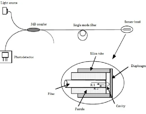
Figure 2.7: Schematic structure of a diaphragm based interferometric sensor

The schematic sturucture of FP acoustic sensor is shown in Figure 2.7. Basically the system includes a laser source, signal processor, bonded by the silica fiber, with the ferrule, the tube, and the diaphragm together to form

an interferometer with a sealed cavity for detecting acoustic emissions [18]. The laser light goes into fiber coupler and propagates through the sensing part consisting of cylindrical ferrule carrying the fiber and the diaphragm forming the FP cavity. A part of the incident light is reflected at the end of the fiber due to the Fresnel reflection. The light transmitted through end of the fiber strikes the diaphragm and experiences a second reflection. These two reflected beams travel back in the same fiber and variously interfere while the cavity length changes due to the acoustic pressure.

2.2.1

Acoustic Wave and Pressure

Acoustic wave is a longitudinal wave involving a sequence of pressure pulses through an elastic medium [28]. The transverse of an acoustic wave depends on the medium which is included in, and owing to this, acoustic wave detections are very essential to examine the concerned material and its physical features. The most general application is highly sensitive microphones besides having other prevalent applications including ultrasound detection, material defect detection, and medical diagnostics. Among all the variety of the applications the principle relies on the information of the acoustic wave behavior in the interested media. The acoustic wave sensors may vary on the frequency range they are operating with.

2.2.2

Hearing Treshold

For acoustic sensing threshold of hearing is also considered. It can be described as minimum sound level for normal hearing of an average person. The inten-sity of the sound required differs for different values of frequency and audible frequency varies from 20 Hz to 20 kHz [28].

Intensity of sound is defined as power of sound per unit area and the refer-ence sound intensity is defined as,

I0 = 10−12W/m2 (2.8)

And the sound intensity level is defined as,

I(dB)= 10log10

I I0

(2.9)

Which is equivalent to 20 µPa under room conditions [5]. According to this reference value, the intensity is usually expressed by a logarithmic ratio instead of the absolute value of pressure or intensity. Sound pressure level (SPL) which is defined for the logarithmic measure of sound intensity or pressure has unit of decibell (dB), can be expressed as the equation below.

Lp = ln( p p0 ) (2.10) Lp = ln( p p0 ) (2.11)

B = 20log10(

p p0

) (2.12)

Since the reference pressure value is taken as 20 uPa which is p0 at 1000 Hz,

the standard threshold of hearing is assumed as 0 dB. Mentioned before, there is a segregation of minimum SPL needed to be heard for different frequencies.

2.2.3

Sensitivity

The pressure responsivity and resolution of a Fabry- Perot interferometric sensor are dependent on the light source, detector, amplifiers and other com-ponents used in the system besides the diaphragm itself.

The finesse is another parameter to define the sensitivity of a Fabry-Perot interferometer. Finesse is a measure of the transmission peak. It can be seen that finesse is directly proportional to reflectivity (R). Finesse is formulized as,

f = π √

R

1 − R (2.13)

Higher reflection coefficients results in higher finesse and narrower trans-mission peaks. It can also be calculated by the ratio of free spectral range, and the full width half maximum (FSR/FWHM). The free spectral range across the optical spectrum is defined as the distance between transmission maximums. Plotting reflectivity vs. finesse allows visualization of the finesse parameter. Figure 2.8 illustrates how finesse value change with reflection coefficient [1].

From the equation above, different finesse values can be calculated from re-flectivity.

Figure 2.8: Ratio of transmitted and incident light intensity as a function of phase difference[1]

Consequently material choise is an important factor to specify the re-flectance of the surface. In this operation reflectivity is assumed to be constant everywhere. Briefly, largest FSR and minimum FWHM values are desired to have high sensitivity, however finesse is limited by the reflection coefficient.

Chapter 3

Mechanical Optimization of

Fiber-Optic Acoustic Sensor

With the development of semiconductor industry, new types of devices can be produced easily and cost-effectively. This innovation revealed microelec-tromechanical systems (MEMS) technology that initiated new manufacturing methods with higher quality. Improvement in silicon etching technology has continued the trend to provide better methods for MEMS sensor fabrication. More recently, the highly directional plasma etching technique was developed to achieve the fast etching rate and a high depth-to-width aspect ratio [29].

While semiconductor micro-machining technology enables high precision micro structures. What makes the silicon micro-machining technique so con-venient is the high control level mechanism. The processes or the technique include deposition of the material required, patterning for desired structure and etching. The rates for deposition can be as low as several angstroms

control for deposition which is feasible for fabricating microphone diaphragm with desired vertical and horizontal dimensions by the lithography methods. Moreover, these methods enable fabricating hundreds of devices at one process. Overall, high control level expedites fabrication and its quality.

3.1

Membrane Mechanics

3.1.1

Membrane Deflection

When the mechanical mode of a diaphragm is considered, it can be modelled as a micromechanical resonator that can be characterized with the resonance frequency and spring constant. The interaction between the differential pres-sure and the diaphragm creates a force on the diaphragm and this results with a dynamic deflection. The pressure is transformed to an electrical signal with the measurement of a secondary sensor. In our case, pressure transforms to a mechanical motion of diaphragm, later to an optical signal in an interferometer and finally the optical signal is converted to an electrical signal through a pho-todiode and an amplifier. In every step of this transformation, fundamental noise sources step in and play a part of evaluating the minimum measurable pressure change.

During dynamic force measurements with micro-mechanical resonators, fundamental fluctuations caused by pressure fluctuations and Brownian mo-tions stand out between fundamental noise sources. Especially in the case the noise level of secondary transduction mechanism is very low, which is our case, the major limiting factor is the Brownian motion. Besides, pressure

fluctuations generated in air can be used for the prediction of the minimum measurable pressure fluctuation through fluctuation-dissipation theorem.

A generalized form of Nyquist equation [30] can be used to evaluate the spectral density of the fluctuating pressure, in other words thermal noise of the acoustic sensor, in units of (P a/√Hz). Alike the measurement of Johnson noise level of a resistance, this fundamental noise level [31] can be calculated in a pressure sensor by the equation:

PN =

p

4kBT R (3.1)

R and PN are the acoustic radiation resistance and RMS amplitude of

pres-sure fluctuation in 1 Hz bandwidth relatively. By using this equation, when noise level is evaluated around 30 kHz under normal circumstances in air, min-imum measurable pressure level is found to be 600 nPa/√Hz. Independently from the technology used for measuring the pressure, this level indicates the minimum noise level of any type of microphone can achieve [32].

Where the spring constant of a micro-mechanical resonator is k, the reso-nance frequency is w0 and the quality factor is Q, the equation for

transfor-mation of force to motion is given below:

H(ω) = F (ω) X(ω) = 1 k 1 1 −ω 2 ω2 0 + iω ω0Q (3.2)

From this equation we can evaluate the Brownian motion spectrum of the resonator,

Sx(ω) =

4kkBT

Qω0

|H(ω)|2, m2/Hz (3.3) In the equation above, the kBT gives the thermal energy which is the

multiplication of Boltzman constant and temperature. We can obtain a clearer form of the equation as follows:

Sx(ω) = 4kBT kQω0(1 − ω2 ω2 0 2 + iω ω0Q 2 ) , m2/Hz (3.4)

Minimum measurable force, which contains the transfer function given in Eq. 3.2, comes out independent from frequency and minimum detectable force limited by Brownian noise can be evaluated with following equation where B is bandwidth. F(min, th) = s 4kkBT B Qω0 (3.5)

In order to adjust the equations above to a dynamic features of a di-aphragm, effective spring constant, resonance frequency and Q must be calcu-lable depending upon geometrical parameters, characteristics of the material (stress, Young’s modulus, Poisson ratio etc.) and air.

For small deflections, the deflection is defined as the elastic response of the diaphragm regarding thin film theory [33]. Deflection, w, of a fixed circular plate under a uniform applied pressure P, is given by,

ω(r) = P a 4 64D[1 − (r a) 2_]2 (3.6)

Where r and a are the radial coordinate and the radius of a circular di-aphragm, respectively. The flexional rigidity, D, is an elastic response of the diaphragm that can be shown as,

D = Eh

3

12(1 − v2₎ (3.7)

Where E, h and v are Youngs modulus, plate thickness and Poissons ratio respectively. In case of the stress is high and motion is defined by the stress instead deflection resistance of the plate, the equation for deflection is given by: ω(r) = P a 2 4σih [1 − (r a) 2 ] (3.8)

3.2

Mechanical Optimization of Membrane

Properties and Fundamental Noise Sources

In case of high stress, where stress of a circular diaphragm dominates elastic deflection and the case of elastic deflection domination, Equations are used to evaluate motion of different center points. Total center motion, wtotal, can be

expressed as a sum of the flexibility of two cases acquired.

1 ωtotal = 1 ωplate + 1 wmembrane (3.9)

In the circumstances, deflection of a diaphragm (motion of the center) under uniformly applied pressure, P, is given by,

ωtotal = P a4 64D 1 1 + a 2_σh D (3.10)

Where D is elastic stiffness of diaphragm given. When harmonic oscilla-tor functions are interrelated with Brownian noise, the motion stated can be expressed in terms of an effective spring constant. If we consider the total pres-sure as intensified applied force to center, the spring constant can be defined by, k = dωtotal d(πa2_{P )} = 1 πa2 dωtotal dP = 16Eh3 3πa2_(1ν2₎(1 + 12a2_{σ(1 − ν}2₎ Eh2 ) (3.11)

The outstanding characteristic is combining the geometric parameters and stress. Hence, it is feasible to evaluate how stiffness of diaphragm change with any stress value. Resonance frequency of diaphragm is needed in order to calculate Brownian motion and minimum measurable pressure value. When spring constant and motion distribution of diaphragms fundamental mode are considered, resonance frequency can be calculated as,

ω0 = 2πf0 = s k mef f = h πa2 s 16E ρ(1 − ν2₎ r 1 + 12a 2_{σ(1 − ν}2₎ Eh2 (3.12)

Where ρ is the mass density. When we consider fluctuation distribution of diaphragms fundamental mode is given by Eq. 6, the equivalent mass, mef f,

can be calculated by the integral given below.

mef f = 2πρh

Z a

0

1 − r2/a2rdr (3.13) At the limit of quantification of Brownian force motion that can be cal-culated, should be also evaluated as well as k and ω0. When air friction and

acoustic propagation are considered as dominant factors, Q multiplier can be estimated by,

Qair = ξ

ω0hρ

Zair

(3.14)

Where ω0 10 is correction factor and Zair =410 Pa s/m is the acoustic

mea-calculate.

In Figure 3.1, by using the equations above, resonance frequency, effec-tive spring constant, minimum detectable force limited by Brownian motion and minimum detectable pressure values are shown as functions of diaphragm radius and stress.

Here, noise of interferometer is defined as Shot noise level that is obtained by 500 uW is impulse power and 50 A/m interferometer sensitivity. Thermal limit, the minimum detectable pressure (600 nPa/sqrt (Hz) around 30 KHz), and threshold of hearing (20µP a) are shown with red lines. In case of stress is low, resonance frequency is still evaluated above 20 kHz (maximum threshold of hearing) when a diaphragm with 500 µ radius in use. As stress decreases, minimum detectable pressure level converges to thermal limit. Calculations for Si3N4 diaphragm with 50 nm thickness are given below.

In order to understand the stress effect on characteristics and measurement limitations of diaphragm, Fig. 2 can be taken as reference. Similarly, resonance frequency, spring constant, minimum detectable force and pressure caused by Brownian noise are shown for 50 nm thick Si3N4 diaphragm and diaphragms

with 50, 100, 200, and 500 µm radius. The results shows the importance of stress control.

Finally, to understand frequency dependence better, minimum pressure value when Q multiplier is around 1, is plotted in Figure 3.3 at different stress levels.

3.2.1

Flat Membrane and MUMPS

In order to get higher pressure detection resolution, reducing the system noise is required. From the above equations, it can be seen that the resolution of the sensor can be adjusted to for different types of applications. The detector, light source, and amplifiers play significant roles on the sensitivity of the sensor. In order to optimize the sensitivity, diaphragms with different designs and materials are tried to be developed. When membrane deflection I discussed, it was seen that geometrical parameters are effective on the detection of acoustic waves by the diaphragm. Hence, with optimized diaphragm radius r, thickness t, and material type by the mathematical model discussed in previous section, desired sensitivity levels can be obtained. It was shown that larger radius and thinner diaphragm imports higher sensitivity, however our aim is to obtain minimized diaphragm with high level of detection. Besides, thinner diaphragm makes the frequency response lower, optimizing the geometrical parameters is a challenge. In order to get different operating ranges and response, material and its geometry can be altered.

In this section we simulate our designs for acoustic sensor diaphragm according to the mathematical model we discussed in the previous section. Hereby, two different models will be examined which are circular flat mem-brane and MUMPS structure memmem-brane.

3.2.1.1 Flat Membrane

In the previous section, membrane deflection mechanism is overviewed. Ac-cording to the mathematical models we tried to verify the results with finite element simulations. In previous section it was shown that resonance frequency can be evaluated with the change of stress value. The change in the stiffness of diaphragm with stress is evaluated and resonance frequency of the diaphragm is also needed to calculate Brownian motion. To understand the stress effect on the characteristics to examine the diaphragm limitations, models are ap-plied for 50 nm thick Si3N4 diaphragm and diaphragms with 50, 100, 200, and

500 µm radius and it was shown the effect of stress on resonance frequency.

We present several models for interferometric acoustic sensor diaphragm do specify the behavior of the resonance frequency change with diaphragm radius and stress values. COMSOL Multi-physics finite element method is employed to simulate our models.

In Figure 3.4 mathematical model and COMSOL simulations comparison for effect of stress on resonance frequency. The calculations and modeling are performed for 100 nm thick Si, and stress values range is 1 Pa to 110P a.

3.2.1.2 Multi-User MEMS

MUMPs (Multi-User MEMS processes) is a commercial program performed by MEMSCAP company [?]. PiezoMUMPS is a subgroup of of MUMPS program, and the cross section of all layers are shown in Figure 3.5 Within this scope we have designed different structures and materials of diaphragms and took the delivery of fabricated membranes.

As part of PiezoMUMPs, our aim was to design membranes with desired characteristics to optimize the Fabry-Perot Interferometric microphone. Thus it was critical to decide upon the parameters of the structures those would be fabricated. In the PiezoMUMPs process, the thicknesses of the layers men-tioned in the fabrication steps, cannot be altered. Thus, for the mechanical optimization other parameters except thickness are optimized for suitable res-onance frequency, spring constant and displacement amplitude. The resres-onance frequency of a diaphragm can be calculated by,

f = 1 2π

p

k/m (3.15)

By using the equations below, spring constant and mass can be calculated for optimum membrane parameters. Spring constant and mass can be evalu-ated by Eqs. 3.16 and 3.17. In addition, resonance frequency can be calculevalu-ated by Eq. 3.18, and Eq. 3.19 gives the displacement amount. E, ρ, R, N, ω and t are Youngs modulus, mass density, radius of diaphragm, number of arms on the diaphragm, width of one arm and film thickness respectively.

m = πR2tρ (3.17) f = 1 2π s Eωt2N4 8π4_R5_ρ (3.18) ∆z = P πR 2_(2πR)3 Eωt3_N4 (3.19)

In consideration of these calculations, diaphragm designs for four different materials were created. Geometrical parameters used in designing are given in Figure 3.6. Five different masks were designed for five different photolithogra-phy steps.

In Figure 3.8 and Figure 3.9, COMSOL simulations for MUMPS diaphragm for Si are shown. Finite element analysis results are agreeable with the math-ematical model. Thus, the designed mask is sent to be fabricated.

Figure 3.1: a) Resonance frequency b) effective spring constant c) minimum detectable force limited by Brownian motion and d) minimum detectable pres-sure values are shown as functions of stress and diaphragm radius for 50 nm thick Si3N4 diaphragm. Here, noise of interferometer is defined as Shot noise

level that is obtained by 500µW impulse power and 50 A/m interferometer sensitivity. Thermal limit, the minimum detectable pressure (600nP a/√Hz ) around 30 kHz), and threshold of hearing 20 µP a (d) are shown with red lines.

Figure 3.2: For 50 nm thick Si3N4 diaphragm with 50, 100, 200, and 500 µm

radius a)Resonance frequency, b) Effective spring constant, c) minimum de-tectable force and d) pressure caused by Brownian noise are shown as functions of stress and radius of diaphragm. Here, noise of interferometer is defined as Shot noise level that is obtained by 500 µW is impulse power and 50 A/m interferometer sensitivity.

Figure 3.3: Noise levels in terms of frequency are shown when Q=1 for 50 nm thick Si3N4 diaphragm with 500 µm radius. a) Brownian motion noise

dependent on frequency and b) The minimum detectable pressure at different stress values are shown for 500µW is impulse power and 50 A/m interferometer sensitivity. Red line indicates thermal limit which is 600 nP a/√Hz.

Figure 3.4: COMSOL simulation results compared with membrane deflection model

Figure 3.6: Geometrical parameters for Si, SiO2, Al and AlN membranes and

Figure 3.7: a)Si Membrane Din = 350 µm Dout = 750 µm t = 1 µm w = 10

µm N= 5, b) SiO2 Din = 350 µm Dout = 750 µm t = 0.2 µm w = 10 µm N=

13, c) AlN Din = 350 µm Dout = 750 µm t = 0.5 µm w = 12 µm N= 6, d)

Figure 3.9: Finite element analysis of Si MUMPS membrane with specified geometrical parameters

Chapter 4

Experimental Process

In the previous chapters, the fundamental theory of the Fabry-Perot interfero-metric acoustic sensor is mentioned in terms of sensitivity and sensor frequency response and noise calculations. This chapter is focusing on the fabrication of the diaphragms for the Fabry-Perot interferometric acoustic sensor with two different methods and designs.

4.1

Fabrication of Flat Membrane

The fabrication of a flat circular diaphragm for fiber-optic microphone with Al2O3 as membrane forming material is feasible with modern microfabrication

techniques. Fabrication process of Al2O3 membrane includes four main steps

namely wafer cleaning, Alumina deposition, photolithography and deep reac-tive ion etching (DRIE). Later the samples are characterized with scanning electron microscope. Figure 4.1 illustrates the fabrication steps of alumina

diaphragms for fiber-optic microphone.

4.1.1

Wafer Cleaning

Before fabrication of the membranes, organic and other contaminations should be removed off in order to deposit our membranes smoothly on the silicon wafer. Intrnsic type 200 µm thick Si wafers are used for diaphragm holders. The wafers are submerged in acetone, methanol and isopropyl alcohol solutions for about 5 minutes for each respectively to remove dusts and organic particles. An additional ultrasonic treatment is used to improve efficiency of removal. Afterwards, sulfuric acid and hydrogen peroxide mixture, H2SO4 : H2O2 (4 :

1), which is called piranha solution, is used to remove off organic contaminants. The wafers are cleaned in piranha solution for about 10 minutes. Later the samples are rinsed with distilled water and dried with nitrogen gun. Since Piranha solution is a strong oxidizing agent, H2O : HF (95 : 5) mixture is

applied to remove the native oxide layer on silicon surface. The wafers are cleaned in HF solution for 3 min. Then, they are rinsed with DI water and dried with N2 gun.

4.1.2

Diaphragm Layer Deposition

The second step of diaphragm fabrication includes deposit alumina layer which forms the diaphragm part. For Al2O3 deposition Atomic Layer Deposition

(ALD) technique is used. ALD is a chemical vapor deposition technique used for many types of semiconductor processes. Since semiconductor industry has been focusing on scaling down, getting high aspect ratio structures also requires

highly conformal coatings. ALD is a key tool to achieve this goal. In this respect ALD is the most reliable deposition technique in terms of conformality among thin film deposition techniques [34]. For the deposition step, Cambridge Nanotech Savannah thermal ALD system is used to grow Al2O3 layer on 200

µm thick Si wafer. 20 nm and 50 nm thick Al2O3 is deposited at 800C to

have lower stress [35]. Prior to the deposition process, 1.4 µm thick AZ5214 photoresist is spun onto backside of the Si wafer for protection.

4.1.3

Photolithography and DRIE

The next step of fabrication is lithography of diaphragm holders, after Al2O3

deposition. Since depth of profile is 200 µm need to be etched, the photoresist type AZ4562 is spun onto the wafer which is 10 µm thick. Thick photoresist also protects the wafer from over-etching. Approximately 30 min post bake is performed to provide DRIE resistance after completion of lithography step. Figure 4.2 illustrates the schematic structure of diaphragm holders photomask used in fabrication.

The design includes four arms carrying the holder in purpose to release the diaphragm from the wafer easily. Arms are designed with two different width which are 20 and 30 um for the event that over-etching that DRIE may cause. Photolithography is executed under the conditions 200 mJ of dose level and soft contact mode. Optical microscope images are shown in Fig. after the process of photolithography and developing. For the development process of AZ4562 includes K400 developer and DI water mixture (1 : 4), and the samples are agitated into the solution for 2-3 minutes.

by ALD. As a key process for MEMS fabrication, deep reactive ion etching (DRIE) is used to etch Si. Being able to achieve high aspect ratio, form com-plex structures isotropically or anisotropically and compatible to photoresist masks are features of DRIE making it an essential process for MEMS.

What makes DRIE different from conventional reactive ion etching tech-niques is a time-multiplexed ICP process. Common name for DRIE for Si etching is Bosch Process [36].In Fig. typical cycle of Bosch process is illus-trated. One cycle of Bosch process employs two or more plasma purges; C4F8

is deposited for sidewall passivation and SF6 is used for etching. Each time

one of these gases is purged into the chamber. These subsequent steps provide vertical sidewalls with high aspect ratio.

DRIE process is performed with STS Inductively Coupled Plasma (ICP) system to etch through the wafers to form the membrane holders and release the membranes. At starting point, Smooth side-wall recipe is used [37]. This standard recipe should end up with smooth side-walls and 1.5 µm per minute etch rate. In our first recipe, the flow rates of C4F8 and SF6 are 100 sccm and

130 sccm respectively. Additionally, O2 plasma is entrained into etch phase.

The recipe consists of a successive 8 seconds etch steps with SF6 and O2 and

12 s side-wall passivation step with C4F8. The plasma power is set at 600 W

and platen coil is set at 20 W. All parameters used in the first recipe is given in Figure 4.5.

After 1 hour process with the recipe given above, samples are cleansed from photoresist with Piranha solution for 5 minutes and rinsed with DI water. Lastly wafers are dried with N2 gun.

Samples are characterized with Scanning Electron Microscopy (SEM). Ac-cording to the SEM images the etch rate for our process is approximately 3.5 µm per minute, however it is seen that Si is over-etched with almost no holder left. The holder arms are couple of microns wide and side-walls are also not vertical as expected.

Since SF6 flow rate, coil and platen powers are key parameters to define

the etch rate, the recipe is then modified with lower SF6 flow rate 90 sccm, coil

power 400 W, and platen power 10 W are utilized in separate runs. Subsequent steps are executed for 1 h as well in order to control the etch rate. Later, etched wafers are characterized from SEM images with more vertical side-walls but still over-etched structures. In Figure 4.7 DRIE parameters effects on etching are summarized.

According to this Table, the recipes are modified with different flow rates and deposition/ etch steps durations. Hence, the latest recipe is improved by setting the C4F8 flow rate at 70 sccm and SF6 flow rate at 80 sccm with 5 s

and 3 s duration respectively. Furthermore O2 flow is added into etch phase

with 5 sccm in order to improve the anisotropic etch. The coil and platen powers are maintained at 400 W and 13 W respectively which provide more controlled but low etch rated DRIE process. The parameters used in improved recipe are given in Table that is also run for 1 hour. The etch rate is 1 µm per minute, means more than 3 hours are needed in order to reach the membrane layer.

Etched wafers with improved recipe are characterized with SEM as well. Figure 4.9 illustrates a cross section and a tilted view of Si wafer Al2O3

de-posited on the backside. Images are captured before removing the photoresist. It is seen that 1 hour run etched 4 µm of the photoresist.

SEM results show one hour run etches approximately 60 µm Si. Although grass effect is observed, it is planned to reduce it by a post process with XeF2.

Moreover the structure shows up with more vertical walls. In order to reach the diaphragm layer, the recipe is run for 2.5 hours continuously with the same structure. Similarly, SEM is used to observe the results and Figure 4.10 indicates long period Bosch process deforms the desired structure.

4.2

Multi-User MEMS (MUMPS)

4.2.1

Fabrication Process

In the fabrication process of Piezo MUMPS, has five main photolithography steps where silicon on insulator (SOI) is used as substrate. In the first step 200 nm thick thermal oxide is grown on SOI, then the lithography takes place with PADOXIDE mask. Reactive ion etching (RIE) is used for etching process. In the second step 0.5 µm thick AlN is grown as piezoelectric layer. In order to have desired structures wet etch is used after photolithography is executed with PZFILM mask. In the third step, PADMETAL mask is used for another lithography step. 20 nm Cr and 1 µm AlN thin films are deposited and the structures are obtained after lift-off operation. Fourth step includes lithogra-phy with SOI mask and Deep Reactive Ion Etching (DRIE) etching which is a Inductively Coupled Plasma (ICP) technique is used for molding. In the last part, devices are coated with a protective layer and backside etched with DRIE method after the lithography with TRENCH mask [38]. The fabrication steps are shown in Figure 4.11.

4.2.2

Post Process

Following the delivery of MUMPs membranes, some post process steps are involved for making them usable in our interferometric-microphone device.

Figure 4.12 shows SEM images of PiezoMUMPS diaphragms after recieved. Because of Si trench layer exist below all diaphragms, it should be removed

is used to remove Si. For the first etch process 25 cycles of XeF2 etch is

performed. As a second step 25 minutes Bosch process is performed, then 15 minutes SF6 etch is done. SEM images of Al, AlN, and SiO2 membranes after

these 3 etch process are shown in Figure 4.13.

4.3

Results

In experimental section, flat and MUMPS membranes are tried to be fabri-cated. Related with ICP optimization, alumina diaphragms could not be re-leased. However, an enhanced optimization of deep reactive ion etching recipe can enable the vertical side-wall etching and release the diaphragms.

PiezoMUMPS diaphragms are designed and custom fabricated. The mem-branes fabricated had desired characteristics, however no signal can be ob-served when utilized in Fabry-Perot interferometric microphone.

Figure 4.2: shows the schematic structure of diaphragm holder obtained by Si wafer etching. There are four sizes of holders those are 100 and 150 µm inner radius and 400 µm outer radius. The outer radius value is constant by the purpose of the diaphragm is planned to be clamped to the ferrule which has also 400 µm radius. Fig. (b) is the image of photo-mask design showing the four structures.

Figure 4.3: Microscope images Si wafer after development a) t=20 µm R1=150

Figure 4.4: A cycle of Bosch process

Figure 4.6: Tilted and top view of Si membrane holders after 1h DRIE run

Figure 4.7: Effects of DRIE process parameters on etch rate, profile, selectivity, grass, breakdown and sidewall [36]

Figure 4.9: Profile and tilted SEM images of Si membrane holders after 1 h run with improved recipe

Figure 4.10: Profile and tilted SEM images of Si membrane holders after 2.5 run with improved recipe

Figure 4.13: SEM images of 3 different types of MUMPS membranes after etching

Chapter 5

Optical Optimization of

Fiber-Optic Interferometric Acoustic

Sensor

5.1

Experimental Design

In order to test fiber optic microphone and verify the models, experimental set up shown in Figure 5.1 was built up for measuring noise levels and sensitivity values.

Experimental setup provides a controlled approaching of glass capillary carrying diaphragm to fiber holder with the aid of motor controlled XY mo-tion platform. Issues involving screw, gap prevent to get bidirecmo-tional sensitive movement as well as the step length is 20 nm in motorized motion.

Interferome-Figure 5.1: a) Setup for experimental study of fiber optic interferometric mi-crophone. b) Schematic demonstration of the same setup

in order to control more sensitive (nm) movements and observe interferometer fringes, a platform glass jacket can be plugged easily on a piezoelectric crys-tal, was fabricated. Thus, PZT control can be performed with high voltage amplifier by computer control directly. Through a speaker not shown on the figure, test signal with desired frequency, magnitude and length can be send to microphone for measuring frequency response. Because of the speaker is not calibrated, ADMP401 Analog Devices MEMS microphone was taken as referance to obtain reliable measurement results. In the experimental setup, ADMP401 placed near fiber optic microphone, is enhanced by 60 gain ampli-fier and the output signal is combined to test control computer via DAQ card. Thus, sensitivity levels of the interferometer can be observed with different phases. FFT spectrum analyzer connected to system, helps determining the signal and noise levels. Analogously, the signals can be digitalized by high-speed DAQ card for extensive and faster measurements. Noise level, signal spectrum and response measurements can be performed by FFT analysis. Q constant and resonance frequency parameters can be evaluated by adapting Brownian noise spectrum to the equations. Ferrule used in pre-studies has

a jacket with 140 µm radius hole. The ferrule with outer radius 1.8 mm, is located by XY platform and glass jacket carrying diaphragm, after fixing the fiber (Figure 5.1). Firstly, positioning is executed by a camera with a mi-croscope manually (Figure 5.2). Afterwards, with the aid of motor controlled mechanism, signal characterizations done with computer program as a function of distance. Necessary scripts are created for automatization.

Figure 5.2: The image of the fiber interferometer for two different location. Distance between fiber and diaphragm can be set around 150 um manually

In our interferometric sensor setup, diaphragms fabricated by silicon etch-ing technology with 50, 100, and 200 nm thickness (Figure 5.4 (b)). Di-aphragms have rectangular shape and each side is 1 mm long. Resonance frequency measurements show that the stress on diaphragms is between 1 Mpa and 10 Mpa.

To minimize the effect of temperature that may cause deflections, two-sided metal coating was executed. Sputtering technique was used to coat Au layers.

Figure 5.3: a) Laser intensity noise is 500 µW impulse and for 1 µA/W gain . b) Relative intensity noise (RIN) level is around 0.2%. This value is 100 times higher than Shot noise level and needed to be removed by a stabilization circuit.

5.2

Characterization Methods and

Measure-ments

Figure 5.6 illustrates that laser intensity fluctuation is around 10 mV for 500 uW impulse and 1 uA/V gain values.

Although the microphone setup was not composed in a noise dampening chamber, background noise can be caused by fan and air conditioning, are among the limiting factors. This noise was measured by the ADMP401 test microphone and results are illustrated in Fig 15.

Test signals were sent to fiber microphone and ADMP401 test microphone and responses are illustrated in Figure 5.8 and Figure 5.9. A commercially used speaker has been used during the frequency response measurements, hence pre-frequency measurements are not accurate. Furthermore, sound detection

Figure 5.4: a) Ferrule and glass jacket that is going to hold the diaphragm b) Microscope image of 50 nm thick Silicon Nitride diaphragm. It became semi-transparent with 15 nm gold coating on both sides.

results show that signal noise performance is slightly less than ADMP401 mi-crophone prototype. In Figure 5.11 the comparison of the noise performances is illustrated.

Figure 5.5: a) Background noise measured with fiber-optic microphone and b) Hello!

Figure 5.6: a) Laser intensity noise is around 10 mV for for 500 µW impulse and 1 µA/V gain values. B) Relative intensity noise (RIN) is at 0.2% level. This value is 100 times greater than Shot noise and need to be reduced by a stabilization circuit

Figure 5.7: Background noise level is 20 mV pp when measured by the ADMP401 test microphone. Considering the existing configuration 1 Pa pres-sure corresponds to 513 mV. Thereby, background noise is approximately 40 mPa pressure level. The background noise is regarded as degradable when fiber microphone is stabilized.

Figure 5.8: Response of ADMP401 to 1 kHz test signal. a) After test signal is over, background noise becomes dominant factor.

Figure 5.9: Response of interferometric microphone to 3 kHz test signal. After test signal is over, background noise becomes dominant factor. Here, 500 µW laser power and 150 µm interferometer gap are used.

Figure 5.10: Frequency responses of ADMP401 and fiber-optic microphone were measured with frequency sweep. In the consequence of sound source was not ideal, unexpected responses was seen especially for low frequencies. Nevertheless, it can be deduced that these two microphones are comparable and they consist the audible band.

Figure 5.11: a) Interferometric microphone and b) ADMP401 responses for sound signals. Compared to fiber-optic microphone ADMP401 has a couple of times larger signal noise ratio (SNR).