Nearest-neighbor based metric functions for indoor scene recognition

NEAREST-NEIGHBOR BASED METRIC

FUNCTIONS FOR INDOOR SCENE

RECOGNITION

a thesis

submitted to the department of computer engineering

and the graduate school of engineering and science

of b

lkent university

in partial fulfillment of the requirements

for the degree of

master of science

By

Fatih C

¸ akır

I certify that I have read this thesis and that in my opinion it is fully adequate, in scope and in quality, as a thesis for the degree of Master of Science.

Prof. Dr. ¨Ozg¨ur Ulusoy (Supervisor)

I certify that I have read this thesis and that in my opinion it is fully adequate, in scope and in quality, as a thesis for the degree of Master of Science.

Assoc. Prof. Dr. U˘gur G¨ud¨ukbay (Co-supervisor)

I certify that I have read this thesis and that in my opinion it is fully adequate, in scope and in quality, as a thesis for the degree of Master of Science.

Prof. Dr. Enis C¸ etin

iii

I certify that I have read this thesis and that in my opinion it is fully adequate, in scope and in quality, as a thesis for the degree of Master of Science.

Asst. Prof. Dr. C¸ i˘gdem G¨und¨uz Demir

Approved for the Graduate School of Engineering and Science:

Prof. Dr. Levent Onural Director of the Graduate School

ABSTRACT

NEAREST-NEIGHBOR BASED METRIC FUNCTIONS

FOR INDOOR SCENE RECOGNITION

Fatih C¸ akır

M.S. in Computer Engineering

Supervisors: Prof. Dr. ¨Ozg¨ur Ulusoy and Assoc. Prof. Dr. U˘gur G¨ud¨ukbay July, 2011

Indoor scene recognition is a challenging problem in the classical scene recogni-tion domain due to the severe intra-class variarecogni-tions and inter-class similarities of man-made indoor structures. State-of-the-art scene recognition techniques such as capturing holistic representations of an image demonstrate low performance on indoor scenes. Other methods that introduce intermediate steps such as identi-fying objects and associating them with scenes have the handicap of successfully localizing and recognizing the objects in a highly cluttered and sophisticated environment.

We propose a classification method that can handle such difficulties of the problem domain by employing a metric function based on the nearest-neighbor classification procedure using the bag-of-visual words scheme, the so-called code-books. Considering the codebook construction as a Voronoi tessellation of the feature space, we have observed that, given an image, a learned weighted distance of the extracted feature vectors to the center of the Voronoi cells gives a strong indication of the image’s category. Our method outperforms state-of-the-art ap-proaches on an indoor scene recognition benchmark and achieves competitive results on a general scene dataset, using a single type of descriptor.

In this study although our primary focus is indoor scene categorization, we also employ the proposed metric function to create a baseline implementation for the auto-annotation problem. With the growing amount of digital media, the problem of auto-annotating images with semantic labels has received significant interest from researches in the last decade. Traditional approaches where such content is manually tagged has been found to be too tedious and a time-consuming process. Hence, succesfully labeling images with keywords describing the semantics is a crucial task yet to be accomplished.

v

Keywords: scene classification, indoor scene recognition, nearest neighbor classi-fier, bag-of-visual words, image auto-annotation.

¨

OZET

˙IC¸ MEKAN TANIMA ˙IC¸˙IN EN YAKIN KOMS¸UYA

DAYALI METR˙IK FONKS˙IYONLAR

Fatih C¸ akır

Bilgisayar M¨uhendisli˘gi, Y¨uksek Lisans

Tez Y¨oneticileri: Prof. Dr. ¨Ozg¨ur Ulusoy ve Do¸c. Dr. U˘gur G¨ud¨ukbay Temmuz, 2011

˙I¸c mekan tanıma, insan yapımı yapıların y¨uksek sınıf i¸ci varyasyonlar ve sınıf arası benzerlikler g¨ostermesi sebebiyle klasik mekan tanıma alanının zorlu bir problemidir. Resmin b¨ut¨unc¨ul temsillerini ¸cıkarmak gibi en ileri mekan tanıma teknikleri i¸c mekanlarda d¨u¸s¨uk performans g¨ostermektedirler. Nesnelerin belirlen-mesi ve ardından onların mekanlarla ili¸skilendirilbelirlen-mesi gibi ara kademeler kullanan di˘ger y¨ontemlerin de olduk¸ca karma¸sık bir ortamda nesnelerin ba¸sarıyla lokalize edilmesi ve tanınması handikapları vardır.

Kodkitabı olarak da bilinen g¨orsel kelimeler k¨umesi tekni˘ginden faydala-narak en yakın kom¸su y¨ontemine dayalı bir metrik fonksiyonu ile bu zorlukların ¨

ustesinden gelebilen bir sınıflandırma y¨ontemi ¨oneriyoruz. Kodkitabı olu¸sumu ¨

oznitelik uzayının mozaikle¸stirilmesi olarak ele alınırsa, verilen bir resim i¸cin, ¨

oznitelik vekt¨orlerinin Voronoi h¨ucrelerinin ortalarına olan ¨o˘grenilmi¸s a˘gırlıklı uzaklıklarının resmin kategorisi i¸cin g¨u¸cl¨u bir g¨osterge oldu˘gunu g¨ozlemledik. Y¨ontemimiz tek bir tanımlayıcı ile bir i¸c mekan testinde en geli¸smi¸s yakla¸sımları ge¸cmekte ve genel bir mekan veri k¨umesinde rekabet¸ci sonu¸clar ¨uretmektedir.

Bu ¸calı¸smada her ne kadar temel sorunumuz i¸c mekan kategorizasyonu olsa da, ¨

onerilen metrik fonksiyonunu otomatik etiketleme problemine de bir temel uygu-lama olu¸sturmak i¸cin kullanıyoruz. Gittik¸ce artan sayısal medya ile, otomatik olarak resimlere anlamlı etiketler ¸cıkarma problemine son on yılda ara¸stırmacılar b¨uy¨uk ilgi g¨ostermi¸slerdir. Bu tarz i¸cerikleri man¨uel olarak etiketlemek gibi ge-leneksel yakla¸sımlar ¸cok bıktırıcı ve zaman harcayıcı olarak de˘gerlendirilmektedir. Bu nedenle resimleri anlamsal olarak ba¸sarıyla a¸cıklayan anahtar kelimelerle otomatik olarak etiketleme, ¸c¨oz¨ulmeyi bekleyen ¨onemli bir sorundur.

Anahtar s¨ozc¨ukler : mekan sınıflandırma, i¸c mekan tanıma, en yakın kom¸su vi

vii

viii

To my mother, father and brother To all loved ones

Anneme, babama ve a˘gabeyime T¨um sevdiklerime

Acknowledgement

I would like to express my sincere gratitude to my supervisors Prof. Dr. ¨Ozg¨ur Ulusoy and Assoc. Prof. Dr. U˘gur G¨ud¨ukbay for their instructive comments, suggestions, support and encouragement during this thesis work.

I am grateful to my jury members Prof. Dr. Enis C¸ etin and Asst. Prof. Dr. C¸ i˘gdem G¨und¨uz Demir for reading and reviewing this thesis. Especially, I thank Muhammet Ba¸stan for his support and endless fruitful discussions about this study and my cousin Mehmet C¸ akır for his motivation. I also would like to thank my officemates Rıfat ¨Ozcan, O˘guz Yılmaz, Erdem Sarıgil and S¸adiye Alıcı for sharing the office with me.

I am grateful to Bilkent University for their financial support during my grad-uate education.

I also would like to thank my friends Ahmet C¸ a˘grı S¸im¸sek, Fahreddin S¸¨ukr¨u Torun, Ziya K¨ostereli, Enver Kayaaslan, Kadir Akbudak and many others not listed here for their caring friendship and motivation. I will miss my housemates Bilal Kılı¸c, Mehmet Kanık, Emrah Parmak and Selim S¨ulek. I wish them all the best in their future academic and professional endeavors.

Finally, most of my gratitude goes to my dearest family. Their profound love, tremendous support and motivation led me to where I am today. To them, I dedicate this thesis.

Contents

1 Introduction 1

1.1 Indoor Scene Recognition . . . 1

1.2 Automatic Image Annotation . . . 4

1.3 Organization . . . 5

2 Related Work 6 2.1 Indoor Scene Recognition . . . 6

2.2 Automatic Image Annotation . . . 8

3 Nearest-Neighbor based Metric Functions 11 3.1 Image Representation . . . 11

3.1.1 The Feature Extraction Process . . . 11

3.1.2 Image Vector Quantization . . . 14

3.2 NNbMF . . . 14

3.2.1 Baseline Problem Formulation . . . 14

3.2.2 Incorporating Spatial Information . . . 16

CONTENTS xi

3.3 NNbMF for Automatic Image Annotation . . . 21

4 Experimental Setup and Results 23 4.1 Image Datasets . . . 23 4.1.1 15-Scenes Dataset . . . 23 4.1.2 67-Indoors Dataset . . . 24 4.2 Experimental Setup . . . 24 4.2.1 Parameter Selections . . . 24 4.2.2 Evaluation Method . . . 25

4.3 Results and Discussion . . . 25

4.4 Evaluation and Results for Auto-annotation . . . 35

4.5 Runtime Performance . . . 36

5 Conclusion and Future Work 38

List of Figures

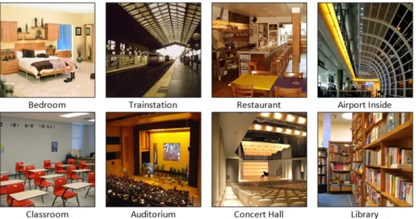
1.1 Some indoor images with their respective classes. . . 2

3.1 Local patches and plotted SIFT descriptors. . . 13

3.2 The Nearest-Neighbor based metric function as an ensemble of multiple classifiers based on the local cues of a query image. . . 16

3.3 Spatial layouts and weight matrix calculation for three different visual words. . . 19

3.4 The flow chart for the testing phase of our method. . . 20

3.5 The flow chart for the training phase of our method. . . 21

4.1 Recognition rates based on different grid size settings. . . 29

4.2 Confusion matrix for the 67-indoor scenes dataset. . . 30

4.3 Confusion matrix for the 15-scenes dataset. . . 31

4.4 Recognition rates based on rankings. . . 32

4.5 Classified images for a subset of indoor scenes. . . 34

4.6 Sample images with respective human annotations from the IAPR dataset. . . 35

List of Tables

4.1 Performance Comparison with Different γ Settings . . . 26

4.2 Performance Comparison with State-of-the-Art Methods . . . 26

4.3 Recognition Rates for each Category (67-Indoors) . . . 33

4.4 Recognition Rates for each Category (15-Scenes) . . . 33

4.5 Annotation performance with different k settings. . . 36

4.6 Performance comparison with a state-of-the-art baseline technique 36

Chapter 1

Introduction

1.1

Indoor Scene Recognition

Scene classification is an active research area in the computer vision community. Many classification methods have been proposed that aim to solve different as-pects of the problem such as topological localization, indoor-outdoor classification and scene categorization [1, 2, 3, 4, 5, 6, 7, 8, 9]. In scene categorization the prob-lem is to associate a semantic label to a scene image. Although categorization methods address the problem of categorizing any type of a scene, they usually only perform well on outdoors [10]. In contrast, classifying indoor images has remained a further challenging task due to the more difficult nature of the prob-lem. The intra-class variations and inter-class similarities of indoor scenes are the biggest barriers for many recognition algorithms to achieve satisfactory perfor-mance on images that have never been seen, i.e., test data. Moreover, recognizing indoor scenes is very important for many fields. For example, in robotics, the perceptual capability of a robot for identifying its surroundings is a highly crucial ability.

Earlier works on scene recognition are based on extracting low-level features of the image such as color, texture and shape properties [1, 3, 5]. Such simple global descriptors are not powerful enough to perform well on large datasets with

CHAPTER 1. INTRODUCTION 2

Figure 1.1: Some indoor images with their respective classes. The intra-class variations and inter-class similarities of indoor scenes are the biggest barriers for many recognition algorithms.

sophisticated environmental settings. Olivia and Torralba [4] introduce a more compact and robust global descriptor, the so-called gist, which captures the holis-tic representation of an image using spectral analysis. Their descriptor performs well on categorizing outdoor images such as forests, mountains and suburban en-vironments but has difficulties recognizing indoor scenes. Borrowing ideas from the human perceptual system, recent work on indoor scene recognition focuses on classifying images by using representations of both global and local image prop-erties and integrating intermediate steps such as object detection [10, 11]. This is not surprising since indoor scenes are usually characterized by the objects they contain. Consequently, indoor scene recognition can be mainly considered as a problem of first identifying objects and then classifying the scene accordingly. Intuitively, this idea seems reasonable but it is unlikely that even state-of-the-art object recognition methods [12, 13, 14], can successfully localize and identify un-known number of objects in cluttered and sophisticated indoor images. Hence, classifying a particular scene via objects becomes yet a more challenging issue.

A solution to this problem is to classify an indoor image by implicitly mod-eling objects with densely sampled local cues. These cues will then give indirect

CHAPTER 1. INTRODUCTION 3

evidence of a presence of an object. Although this solution seems contrary to the methodology of recognizing indoor scenes by the human visual system, i.e., explicitly identifying objects and associating them with scenes, it provides a suc-cessful alternative by bypassing the drawbacks of trying to localize objects in highly intricate environments. The most successful and popular descriptor that captures the crucial information of an image region is the Scale-Invariant Feature Transform (SIFT) [15, 16]. This proposes the idea that SIFT-like features ex-tracted from images of a certain class may have more similarities in some manner than those extracted from images of irrelevant classes. This similarity measure can be achieved by first defining a set of categorical words (the so-called visual words) for each class and then using a learned metric function to measure the distance between local cues and these visual words.

It is very well known in the machine learning community that there is no superior (or inferior) classification method given that no prior assumptions are made about the nature of the problem domain (as described by the No Free Lunch Theorem [17]). Classification methods may be preferred for several rea-sons including their computational complexity, the assumptions they make about the underlying data and their overall competence in high-dimensional space. In this particular problem domain of classfying indoor images, we introduce a novel non-parametric weighted metric function with a spatial extension based on the approach described in [18]. In their work, Bolman et al. show that a Nearest-Neighbor (NN) based classifier which computes direct image-to-class distances without any quantization step achieves performance rates among the top lead-ing learnlead-ing-based classifiers. We show that a NN-based classifier is also well suited for categorizing indoor scenes because: i) It incorporates image-to-class distances which is extremely crucial for classes with high variability; ii) Consid-ering the insufficient performance of state-of-the-art recognition algorithms on a large object dataset [12], it successfully allows classifying indoor scenes directly from local cues without incorporating any intermediate steps such as categorizing via objects; iii) Given a query image, it allows ranked results and thus can be employed for a preprocessing step to successfully narrow down the size of possi-ble categories for subsequent analyses. Bolman et al. also show that a descriptor

CHAPTER 1. INTRODUCTION 4

quantization step, i.e., codebook generation, severely degrades the performance of the classifier by causing information loss in the feature space. They argue that a non-parametric method such as the Nearest-Neighbor classifier has no training phase as the learning-based methods do to compensate for this loss of infor-mation. They evaluate their approach on Caltech101 [19] and Caltech256 [20] datasets, where each image contains only one object and maintains a common position, and on the Graz-01 dataset [21], which has three classes (bikes, persons and a background class) with a basic class vs. no-class classification task. On the other hand, for a multi-category recognition task of scenes where multiple objects co-exist in a highly cluttered, varied and complicated form, we observe that our NN-based classifier with a descriptor quantization step outperforms the state-of-the-art learning-based methods. The additional quantization step allows us to incorporate spatial information of the quantized vectors, and more im-portantly, it significantly reduces the performance gap between our method and other learning-based approaches. It is computationally inefficient for a straight-forward NN-based method without a quantization step to perform classification, considering the datasets with large number of training images.

1.2

Automatic Image Annotation

Auto-annotation is generally incorporated into image retrieval (IR) systems. Pre-viously many content based IR systems allowed example, query-by-sketch or similar query types for searching and retrieving related images. But most users are not familiar with such inputs or it is simply to cumbersome for a user to define a query. Hence it was quickly realized the need for semantic labels describing the content of the images. The traditional solution is to manually associate such semantic keywords to images with the guidance of an application expert. However with growing collections of user-provided visual content this traditional approach has been found to be too tedious and expensive. Hence this issue generated significant interest in the problem of automatically labelling words that describe semantic meanings. A recent review about image retrieveal can be found in [22]. In this study, we also employ the proposed metric function

CHAPTER 1. INTRODUCTION 5

to create a baseline implementation for the particular problem.

1.3

Organization

The rest of this paper is organized as follows: Section 2 discusses related work. In Section 3 we describe the framework of our proposed method. We present experimental results and evaluate the performance in Section 4. Section 5 gives conclusions and future work.

Chapter 2

Related Work

2.1

Indoor Scene Recognition

Earlier works on scene classification are based on extracting low-level features of the image such as color, texture and shape properties. Szummer and Picard [1] use such features to determine whether an image is an outdoor or an indoor scene. Vailaya et al. [3] use color and edge properties for the city vs. landscape classification problem. Ulrich and Nourbakhsh [5] employ color-based histograms for mobile robot localization. Such simple global features are not discriminative enough to perform well on a difficult classification problem, such as recognizing scene images. To overcome this limitation, Olivia and Torralba [4] introduce the gist descriptor, a technique that attempts to categorize scenes by capturing its spatial structure properties, such as the degree of openness, roughness, natu-ralness, using spectral analysis. Although a significant improvement over earlier basic descriptors, it has been shown in [10] that this technique performs poorly in recognizing indoor images. One other popular descriptor is SIFT [16]. Due to its strong discriminative power even under severe image transformations, noise and illumination changes, it has been the most preferred visual descriptor in many scene recognition algorithms [6, 7, 23, 24, 25].

Such local descriptors have been successfully used with the bag-of-visual words

CHAPTER 2. RELATED WORK 7

scheme for constructing codebooks. This concept has been proven to provide good results in scene categorization [25]. Fei-Fei and Perona [24] represent each category with such a codebook and classify scene images using Bayesian hierar-chical models. Lazebnik et al. [7] use the same concept with spatial extensions. They hierarchically divide an image into sub-regions, which they call the spatial pyramid, and compute histograms based on quantized SIFT vectors over these regions. A histogram intersection kernel is then used to compute a matching score for each quantized vector. The final spatial pyramid kernel is implemented as concatenating weighted histograms of all features at all sub-regions. The tra-ditional bag-of-visual words scheme discards any spatial information; hence many methods utilizing this concept also introduce different spatial extensions [7, 26].

Bosch et al. [27] present a review of the most common scene recognition methods. However, recognizing indoor scenes is a more challenging task than recognizing outdoor scenes, owing to severe intra-class variations and inter-class similarities of man-made indoor structures. Consequently, this task has been in-vestigated separately within the general scene classification problem. Quattoni and Torralba [10] brought attention to this issue by introducing a large indoor scene dataset consisting of 67 categories. They argue that together with the global structure of a scene which they capture via the gist descriptor, the presences of certain objects described by local features are strong indications of its category. Espinace et al. [11] suggest using objects as an intermediate step for classifying a scene. Such approaches are coherent with the human vision system since we identify and characterize scenes by the objects they contain. However, with the state-of-the-art object recognition methods [12, 13, 14, 28], it is very unlikely to successfully identify multiple objects in a cluttered and sophisticated environ-mental setting. Instead of explicitly modeling the objects, we can use local cues as indirect evidence for their presence and thus bypass the drawbacks of having to successfully recognize them, which is a very difficult problem considering the intricate nature of indoor scenes.

CHAPTER 2. RELATED WORK 8

2.2

Automatic Image Annotation

One of the earliest papers about auto-annotation is [29]. In this work the authors consider the annotation of an image as a region-keyword association problem (co-occurance of regions and words). They geometrically partition the image and form a feature descriptor for each partitioned part. These partial images (re-gions) are considered to inherit all the tags of the original image, afterwards they vector quantize all regions of all the training images to produce clusters similar to the codebook generation step widely used in the computer vision literature. Given the centroids of the clusters, they estimate the likelihood (conditional den-sity) of each word by accumulating the frequencies of it. After estimating the likelihoods of all the keywords, a test image can be auto-annotated by: i) Geo-metrically partitioning into sub-images; ii) Extracting the feature descriptors of all sub-images and finding the nearest centroids to them; iii) Taking the average of the likelihoods associated with the centroids and obtaining the top k keywords having the largest average density value. They tested their approach on a mul-timedia encyclopedia. In literature this approach is known as the co-occurence model. Duygulu et al. [30] also approaches the auto-annotation problem from a co-occurence perspective where keywords are assigned to image regions (blobs). They first segment images using the popular Normalized cut algorithm [31]. Af-terwards they cluster the segmented region representations to produce ‘blobs’. A lexicon is then constructed which is described as a probability table holding the probability estimations of the blob-keyword translations. Given a test image, it is first segmented and the segmented regions is then quantized into blobs. Fi-nally, each region is annotated with the most likely word. In the literature this approach is named as the translational model.

Jeon et al. [32] introduced the relevance model anagolous to a cross-lingual retrieval problem. Instead of finding one-to-one occurences between blobs and words, they consider assigning words to the whole image by using a joint prob-abilistic distribution association scheme. Lavrenko et al. [33] further improved this method by directly modeling continuous features instead of quantizing (clus-tering) the regions into a discrete vocabulary. Feng et al. [34] showed improved

CHAPTER 2. RELATED WORK 9

performance when the regions were extracted using rectangular grids instead of a segmentation procedure and by modeling the annotation data with multiple-Bernoulli distributions instead of a multinomial model. They argue that the probability mass is splitted among the annotated data for an image with the latter probabilistic model which is infact an incorrect approach to take consider-ing a perfect annotation. Carneiro and Vasconcelos [35] demonstrated a super-vised learning approach for auto-annotation. Their technique learns the class-conditional densities P(x∣w)(x∣i) where each word (w) is considered as a distinct

class and x is a feature vector that represents the concept in an image. Since extracting the feature vector that solely captures a concept in a training image is cumbersome, they adopt a Multiple Instance Learning scheme where the con-ditional densities is estimated by using all the available training images that are annotated with the corresponding word. They argue that the distribution of the concept follows a distinct pattern while the background is uniformly distributed. The densities are modeled with mixture of Gaussians.

Makadia et al. [36] argue that although many techniques have successfully addressed the problem they all lacked any comparison with a simple baseline measure. They asserted that in the absence of such a baseline method it is hard to justify the need for using complex models and training processes. They have introduced a simple propagation model where given an un-annotated query image, the most relevant training images are retrieved using a nearest-neighbor classifier with simple color and texture features. Afterwards, they label the test image using a simple transfer algorithm with the annotations of the training images which are retrieved. They outperform state-of-the-art methods and hence conclude the need for justification of comparing complex methods with a simple baseline technique. Guillaumin et al. [37] improve this propagation model by integrating a metric learning mechanism to determine the weights of the retrieved training images which are consequently used in the auto-annotation process for a test image.

Another notable paper in this problem domain is [38]. In their study, the authors propose a novel Conditional Random Field (CRF) model for semantic context modeling for the auto-annotation problem. CRF [39] has been used to model dependencies of certain sites such as spatial and semantic dependencies and

CHAPTER 2. RELATED WORK 10

has started to increase further attention from the machine learning community. The CRF model has been adopted in [38] in which the semantics, i.e., annotation labels, are considered to have dependencies. Truly certain concepts co-occur frequently in an image dataset, for instance a ‘car’ and a ‘road’ occur more generally than a ‘car’ and a ‘bird’. Thus the authors integrate this ‘contextual’ information by using a novel CRF model. Their paper is the state-of-the-art regarding auto-annotation. Another interesting fact is that such dependencies can also be considered in the scene recognition domain. Certain visual words tend to occur more frequently, hence incorporating this information would likely to boost the performance rate for a categorization method.

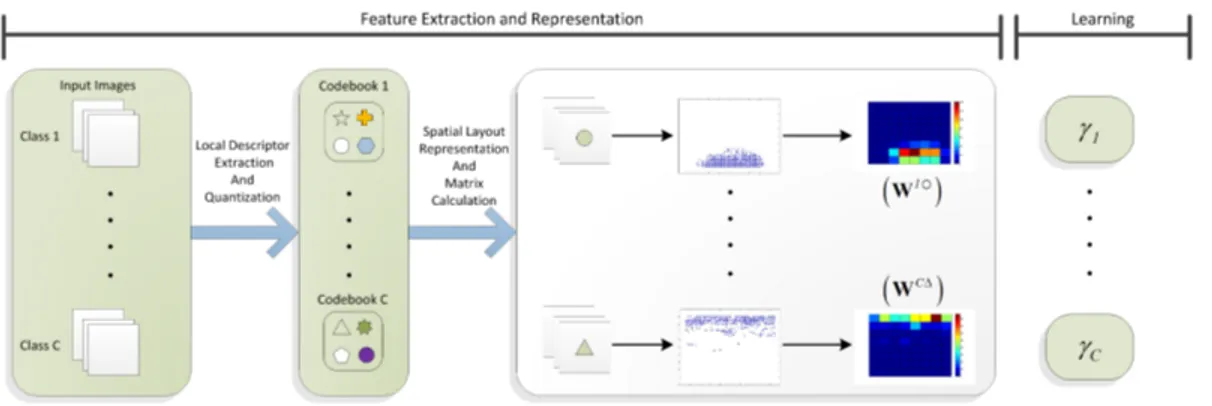
Chapter 3

Nearest-Neighbor based Metric

Functions

In this chapter, we discuss about the proposed approach to classify indoor scenes and to provide a baseline for automatically annotating images. We begin our discussion by describing the feature descriptor we employed to model the local cues of images and the vector quantization procedure undertaken to construct a set of visual words which has proven its effectiveness in the classification literature. Then, we discuss the proposed Nearest-Neighbor based Metric Function (NNbMF) method by first providing the baseline formulation and then extending the metric to incorporate the spatial information of visual words. This treatment is based on the indoor scene recognition problem. Finally, we focus on how to utilize the metric function for annotation purposes.

3.1

Image Representation

3.1.1

The Feature Extraction Process

To consider the image itself as the input data to a classification procedure is gen-erally deemed to be redundant mostly because of the high-dimensional feature

CHAPTER 3. NEAREST-NEIGHBOR BASED METRIC FUNCTIONS 12

space it results in. This redundancy has shown to have a larger impact with nearest-neighbor based search methods [40]. The effects of high dimensionality are referred by the curse of dimensionality term and many dimension reduction techniques have been proposed in the literature to avoid the negative impacts. Given input data, a feature extraction process can also be considered as a di-mensionality reduction technique that produces a reduced set of features. This set of features, also named as a feature vector or descriptor, is then the repre-sentation of the original data in a lower dimensional space. Among many feature extraction techniques, the ones that have certain invariance properties and show robustness to changes in image scale, illumination and noise are more favorable. This transformation process can be applied globally, i.e. to the whole image, yielding a single representative feature vector or locally resulting a set of feature vectors describing the image.

Formally, let us denote the transformation process with the mapping function Φ. Given an image x ∈ X the transformation Φ ∶ X → RD _{yields a global}

descriptor of the image where D denotes the dimensionality of the feature. An example of a global feature vector is the GIST descriptor [4]. If Φ ∶ X → RN ×D then the image is described by a set of feature vectors which generally is obtained from local patches (areas) of an image. The most successful and popular local descriptor is the Scale-Invariant Feature Transform (SIFT) [15, 16]. Not all patches may be used in the tranformation process. Interest point detectors try to detect the salient patches which are considered to be more crucial in classification; such as edges, corners and blobs in an image. Two of the most celebrated detectors are the Harris affine region detector detector [41] and Lowe’s DoG (Difference of Gaussians) detector [42]. After the detection stage, the SIFT descriptor is calculated from a certain scale of the interest point. Although interest point detectors obtain the salient regions in an image, it has been shown that using densely sampled SIFT vectors in a recognition framework demonstrates higher performance [43].

CHAPTER 3. NEAREST-NEIGHBOR BASED METRIC FUNCTIONS 13

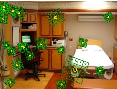
(a) A number of plotted SIFT descriptors on a hospital room image. The interest points are detected using Lowe’s DoG detector.

(b) Plotted SIFT descriptor on a local patch. Notice that there are 4×4 spatial and 8 orientation bins. SIFT transforms this local patch into a 128-dimensional vector.

CHAPTER 3. NEAREST-NEIGHBOR BASED METRIC FUNCTIONS 14

3.1.2

Image Vector Quantization

In statistical text retrieval, a document is represented by a vector composed of frequencies of words in the document. These words are obtained by parsing docu-ments, stemming for removing derivations and rejecting the most frequent words that intuitively have no representative power. Similarly in the case of image analysis, we consider an image as a document and the local patches described by feature descriptors as (candidate) visual words. The equivalent parsing step of text retrieval in the image domain is the feature extraction process. After obtain-ing a set of feature vectors from trainobtain-ing images we apply a quantization step by using a clustering method for similar purposes of stemming in text retrieval. The set of formed quantized vectors, i.e. visual words, is often termed as a dictionary or codebook. Considering a dataset with multiple classes, if the training images in which features are extracted are randomly chosen over all classes, the final visual words are to be representative for all images in the dataset (a global codebook). In such cases images are generally represented by a frequency histogram of the words. On the other hand if a codebook is generated for each class using the respective images only, the codebook is said to be local in which its ‘words’ only describe that particular class.

A concise and formal treatment of the procedure is given in the next section.

3.2

NNbMF

3.2.1

Baseline Problem Formulation

The celebrated bag-of-visual words paradigm introduced in [44] has become com-monplace in various image analysis tasks. It has been proven to provide powerful image representations for image classification and object/scene detection. To summarize the procedure, consider X to be a set of feature descriptors in D-dimensional space, i.e., X= [x1, x2, . . . , xL]

T

∈ RL×D_{. A vector quantization or}

CHAPTER 3. NEAREST-NEIGHBOR BASED METRIC FUNCTIONS 15

by applying K-means clustering to set X to minimize the cost function

J= K ∑ i=1 L ∑ l=1 ∥ xl− vi∥2 (3.1)

where the vectors in V = [v1, v2. . . , vK] T

correspond to the centers of the Voronoi cells, i.e., the visual words of codebook V, and ∥ ⋅ ∥ denotes the L2

-norm. After forming a codebook for each class using Equation (3.1), a set Xq = [x1, x2, . . . , xN]

T

denoting the extracted feature descriptors from a query image can be categorized to class c by employing the Nearest-Neighbor classifi-cation function y ∶ RN ×D → {1, . . . , C} given as

y(Xq) = argmin c=1,...C ⎡⎢ ⎢⎢ ⎢⎢ ⎢⎢ ⎢⎢ ⎢⎣ N ∑ n=1 ∥ xn− NNc(xn) ∥ ´¹¹¹¹¹¹¹¹¹¹¹¹¹¹¹¹¹¹¹¹¹¹¹¹¹¹¹¹¹¹¹¹¹¹¹¹¹¹¹¹¹¹¹¹¹¹¹¹¹¹¹¹¹¹¹¹¹¹¹¹¹¹¹¹¹¸¹¹¹¹¹¹¹¹¹¹¹¹¹¹¹¹¹¹¹¹¹¹¹¹¹¹¹¹¹¹¹¹¹¹¹¹¹¹¹¹¹¹¹¹¹¹¹¹¹¹¹¹¹¹¹¹¹¹¹¹¹¹¹¹¹¶ h(⋅∣θc) ⎤⎥ ⎥⎥ ⎥⎥ ⎥⎥ ⎥⎥ ⎥⎦ (3.2)

where N Nc(x) denotes the nearest visual word of x, i.e., the nearest Voronoi cell

center, in the Voronoi diagram of class c, yi∈ {1, . . . , C} refers to class labels and

h(⋅ ∣θc) denotes a combination function with the parameter vector θc associated

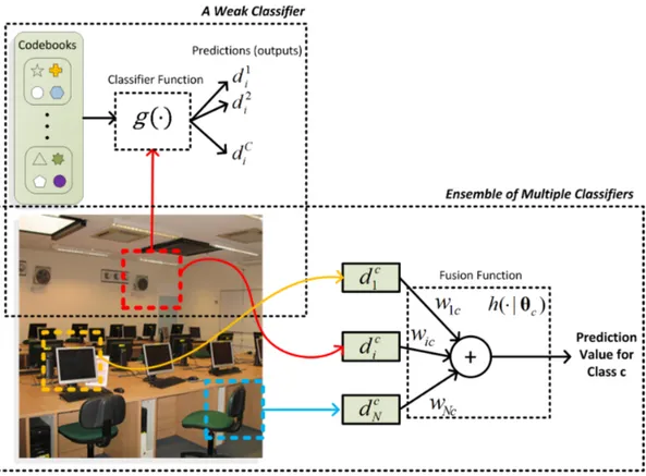
with class c. Intuitively, Equation (3.2) can be considered as an ensemble of mul-tiple experts based on the extracted descriptor set Xq. In this ensemble learning

scheme there are ∣Xq∣ weak-classifiers and h ∶ RN → R is a fusion function to

combine the outputs of such experts. This large ensemble scheme is very suitable for the particular problem domain where each scene object, implicitly modeled by local cues, provides little discriminative power in the classification objective but in combination they significantly increase the predictive performance.

From this perspective, given a query image, assume N base-classifiers cor-responding to the extracted descriptor set Xq = [x1, x2, . . . , xN]T. Let Vc =

[vc1, vc2. . . , vcK] T

and dc

i be the codebook and the prediction of base classifier

g(xi, Vc) =∥ xi− NNc(xi) ∥ for class c, respectively. Taking dci = g(xi, Vc), the

final prediction value for the particular class is then

h(dc 1, dc2, . . . , dcN∣θc) = N ∑ n=1 ωncdcn (3.3) where θc = [ω1c, . . . , ωN c] T

denotes the parameters of the fusion function asso-ciated with class c. Note that θc = 1, ∀c ∈ {1, . . . , C} in Equation (3.2). In

CHAPTER 3. NEAREST-NEIGHBOR BASED METRIC FUNCTIONS 16

Figure 3.2: The Nearest-Neighbor based metric function as an ensemble of mul-tiple classifiers based on the local cues of a query image. Each local cue can be considered as a weak classifier that outputs a numeric prediction value for each class. The combination of these predictions can then be used to classify the image.

the next section, we will use spatial information of the extracted descriptors to determine the parameter vector set θ = {θ1, . . . , θC}. Figure 3.2 illustrates this

concept. It should be noted that Equation (3.2) does not take into account un-quantized descriptors, as in [18]. There is a trade-off between information loss and computational efficiency because of the quantization of the feature space.

3.2.2

Incorporating Spatial Information

The classic bag-of-visual words approach does not take into account spatial information and thus loses crucial data about the distribution of the feature descriptors within an image. Hence, this is an important aspect to consider when working to achieve satisfactory results in a classification framework. We

CHAPTER 3. NEAREST-NEIGHBOR BASED METRIC FUNCTIONS 17

incorporate spatial information as follows. Given extracted descriptors in D-dimensional space, X = [x1, x2, . . . , xL]

T

∈ RL×D _{and their spatial locations}

S = [(x1, y1) , (x2, y2) , . . . , (xL, yL)], during the codebook generation step we

also calculate their relative position with respect to the corresponding image boundaries from which they are extracted. Hence their relative locations are S′ = [(x′ 1, y ′ 1) , (x ′ 2, y ′ 2) , . . . , (x ′ L, y ′ L)] = [( x1 w1, y1 h1) , ( x2 w2, y2 h2) , . . . , ( xL wL, yL hL)] , where

the (w1, h1) , (w2, h2) , . . . , (wL, hL) pairs represent the width and height values

of the corresponding images. After applying clustering to the set X, we obtain the visual word set V as described in the previous section. Since similar feature descriptors of X are expected to be assigned to the same visual word, their corre-sponding coordinate values described in set S′ _{should have similar values. Figure}

3.3 shows the spatial layout of the descriptors assigned to several visual words. To incorporate this information into Equation (3.2), we consider the density esti-mation methods which are generally used for determining unknown probabilistic density functions. It should be noted that we do not consider a probabilistic model; thus obtaining and using a legitimate density function is irrelevant in our case. We can assign weights for each grid on the spatial layout of every visual word using a histogram counting technique (cf. Figure 3.3). Suppose we geomet-rically partition this spatial layout into M × M grids. Then for the fth _visual

word of class c, vcf, the weight of a grid can be calculated as

Wcf = [wcf_ij] = k

N (3.4)

where k is the number of descriptors assigned to vcf that fall into that particular

grid and N is the total number of descriptors assigned to vcf. During the

classifi-cation of a query image, the indices i, j correspond to the respective grid loclassifi-cation of an extracted feature descriptor. An alternative way for defining weights is to first consider Wcf = [wcf

ij] = k, then scale this matrix as

Wcf ′ = [w cf ij] max(Wcf) (3.5)

where max(⋅) describes the largest element. Equation (3.5) does not provide weight consistency of the visual words throughout a codebook. It assigns larger weights to visual words that have a sparse distribution in the spatial layout while attenuating the weights of the visual words that are more spatially compact. The

CHAPTER 3. NEAREST-NEIGHBOR BASED METRIC FUNCTIONS 18

choice of a weight matrix assignment is directly related to the problem domain; as we have found Equation (3.4) more suitable for the 67-indoor benchmark and Equation (3.5) suitable for the 15-scenes benchmark.

We calculate the weight matrices for all visual words of every codebook. The function h(⋅∣θc) described in Equation (3.2) now can be improved as

N

∑

n=1

(1 − γcWcf_ij) × ∥ xn− NNc(xn) ∥ (3.6)

where N Nc(xn) ≡ vcf. The parameter set now includes the weight matrices

associated with each visual word of a codebook, i.e., θc= [Wc1, Wc2, . . . , WcK].

Obviously γcfunctions as a scale operator for a particular class, e.g., if γc = 0 then

the spatial location for class c is entirely omitted when classifying an image, i.e., only the sum of the descriptors’ Euclidean distance to their closest visual words is considered. This scale operator can be determined manually or by using an optimization model. Now, given codebook c, assume a vector dc∈ RN _{that holds}

the predictions of every extracted descriptor xn of a query image as its elements;

i.e., dc

n = g(xn, Vc) =∥ xn − NNc(xn) ∥, where n ∈ {1, . . . , N} corresponds to

extracted descriptor indices and N Nc(xn) refers to the nearest visual word to xn

(NNc(xn) ≡ vcf). αcn denotes the corresponding spatial weights assigned to dcn;

i.e., αc

n = γcWcfij. Referring to the vector of these spatial weights as αc ∈ RN,

Equation (3.6) can now be redefined as(1−αc)⋅dc_{and an image can be classified}

to class c by using the function

y(Xq) = argmin c=1,...C ⎡⎢ ⎢⎢ ⎢⎢ ⎢⎢ ⎣ (1 − αc) ⋅ dc ´¹¹¹¹¹¹¹¹¹¹¹¹¹¹¹¹¹¹¹¹¹¹¹¹¹¹¹¸¹¹¹¹¹¹¹¹¹¹¹¹¹¹¹¹¹¹¹¹¹¹¹¹¹¹¹¹¶ h(⋅ ∣θc) ⎤⎥ ⎥⎥ ⎥⎥ ⎥⎥ ⎦ (3.7)

Consider an image i that belongs to class j with an irrelevant class k. We would like to satisfy the inequalities (1 − αj_i)T dj_i < (1 − αk

i) T

dk

i. Given i training

images and j classes, we specify a set of S = i × j × (j − 1) inequality constraints where k= j − 1. Since we will not be able to find a scale vector that satisfies all such constraints, we introduce slack variables, ξijk, and try to minimize the sum

of slacks allowed. We also aim to select a scale vector γ so that Equation (3.6) remains as close to Equation (3.2) as possible. Hence we minimize the Ln−norm

CHAPTER 3. NEAREST-NEIGHBOR BASED METRIC FUNCTIONS 19

(a)

(b)

(c)

Figure 3.3: Spatial layouts and weight matrix calculation for three different visual words. The left sides of (a), (b) and (c) represent the spatial layouts of the visual words that themselves represent the relative positions of the extracted descriptors to their image boundaries. These layouts are then geometrically partitioned into MM bins and a weight matrix W is computed as shown on the right sides of (a), (b) and (c).

CHAPTER 3. NEAREST-NEIGHBOR BASED METRIC FUNCTIONS 20

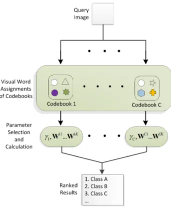
Figure 3.4: The flow chart for the testing phase of our method.

of γ. Consequently, finding the scale vector γ= [γ1, . . . , γj] can now be modeled

as an optimization problem as follows: min ∥ γ ∥n+ ϕ∑ i,j,k ξijk subject to ∀ (i, j, k) ∈ S ∶ (−αj i) T dj_i + (αk i) T dk i < dki − d j i + ξijk ξijk≥ 0 , γ ≥ 0 (3.8)

where ϕ is a penalizing factor. We choose n from{1, 2}, resulting in linear and quadratic programming problems, respectively.

3.2.2.1 LP vs. QP

One may prefer the L2−norm, since sparsity is not desirable in our case due to

the fact that sparse solutions may heavily bias categories associated with large scale weights. An alternative model is to define one weight value associated with

CHAPTER 3. NEAREST-NEIGHBOR BASED METRIC FUNCTIONS 21

Figure 3.5: The flow chart for the training phase of our method.

all categories. This model is less flexible but it prevents a possible degradation in recognition performance caused by sparsity. The scale vector can also be manually chosen. Figures 3.4 and 3.5 depict the testing and training phase of the proposed method, respectively.

3.3

NNbMF for Automatic Image Annotation

In contrast with a regular classification problem where each instance exclusively belongs to a single class, there could be more than one semantic label associated with an image in an annotation domain (we consider semantic labels to be anal-ogous to the classes of a classification framework). As a result the set of visual words constructed for a class in the two domains implicate slightly different mean-ings. In a recognition framework the set of visual words are solely representatives of that particular class whereas in the annotation domain where instances belong to multiple classes it is hard to distinguish the visual words that truly describe the semantic concept. One way to avoid this situation is to assign larger weights to visual words that we somehow believe is more representative to that particular concept. The parameters θc= [ω1c, . . . , ωN c]

T

of the fusion function in Equation (3.3) then holds such weights. However the procedure of calculating the weights is left for future work as well as the option of incorporating spatial information. Consider the set Xq = [x1, x2, . . . , xN]

T

denoting the extracted feature descrip-tors from the image to be annotated, in Section 3.2.2 we assumed a vector dc∈ RN

CHAPTER 3. NEAREST-NEIGHBOR BASED METRIC FUNCTIONS 22

that holds the predictions of every extracted descriptor xn of a query image as its

elements; i.e., dc

n= g(xn, Vc) =∥ xn− NNc(xn) ∥, where n ∈ {1, . . . , N} describes

the extracted descriptor indices and c∈ {1, . . . , C} the semantic labels (classes). Let us define yet another vector δ ∈ RC _{where δ}

c=∥ dc ∥1, to annotate the

im-age with the extracted descriptor set Xq we solve the following binary integer

programming problem min y⋅ δ subject to ∑ c yc= k yc= {0, 1} ∀c = 1, . . . , C (3.9)

where k determines the number of labels for annotation and ∥ ⋅ ∥₁ denotes the L1-norm. Basically with the above optimization procedure we find the classes

Chapter 4

Experimental Setup and Results

In this chapter, we first present the experimental setup and results of our NN-based metric function for the indoor scene recognition task on the 15 scenes [7] and 67 indoor scenes datasets [10]. We then describe our setup and present results for the annotation problem in the subsequent section. Finally, we give information about the runtime performance of our procedure.

4.1

Image Datasets

4.1.1

15-Scenes Dataset

The 15-scenes dataset contains 4485 images spread over 15 indoor and outdoor categories containing 200 to 400 images each. We use the same experimental setup as in [7] and randomly choose 100 images per class for training, i.e., for codebook generation and learning the scale vector γ, and use the remaining images for testing.

CHAPTER 4. EXPERIMENTAL SETUP AND RESULTS 24

4.1.2

67-Indoors Dataset

The 67-indoor scenes dataset contains images solely from indoor scenes with very high intra-class variations and inter-class similarities. We use the same experimental setup, as in [10] and [45]. Approximately 20 images per class are used for testing and 80 images per class for training.

4.2

Experimental Setup

4.2.1

Parameter Selections

In our solution, we use two different scales of SIFT descriptors for evaluation. For the 15-scenes dataset, patches with bin sizes of 6 and 12 pixels are used, and for the 67-indoor scenes dataset, the bin sizes are selected as 8 and 16 pixels. The SIFT descriptors are sampled and concatenated at every four pixels and are constructed from 4×4 grids with eight orientation bins (256 dimension in total). The training images are first resized to speed the computation and to provide scale consistency. The aspect ratio is maintained, but all images are scaled down so their largest resolution does not exceed 500 and 300 pixels and the feature space is clustered using K-means into 500 and 800 visual words, for the 67-indoor scenes and 15-scenes datasets, respectively. We use 100K SIFT descriptors extracted from random patches to construct a codebook.

The spatial layout of each visual word from each category is geometrically partitioned into M× M bins and a weight matrix is formed for each visual word from Equation (3.4) and Equation (3.5). Several settings are used to determine the scale vector γ. We first consider assigning different weights to all categories (γ ∈ RC). We find the optimal scale vector by setting n = {1, 2} in Equation (3.8)

and solving the corresponding optimization problem. We also use another setting for the optimization model where we assign the same weight to all categories (γ ∈ R). Alternatively, we select the scale parameter manually.

CHAPTER 4. EXPERIMENTAL SETUP AND RESULTS 25

The constraints in Equation (3.8) are formed as described in the previous section with 10 training images per class. The rest of the training set is used for codebook construction. The subset of the training images used for parameter learning is also employed as the validation set when manually tuning the scale parameter to find its optimal value. The value that yields the highest performance for this validation set is then selected for our method.

4.2.2

Evaluation Method

The performance rate is calculated by the ratio of correctly classified test images within each class. The final recognition rate is the total number of correctly classified images divided by the total number of test images used in the evaluation.

4.3

Results and Discussion

Table 4.1 shows recognition rates for both datasets with different scale vector settings. Baseline and Baselinef ull refer to the method when Equation (3.2) is

used (no spatial information is incorporated). The difference is that Baselinef ull

uses all available training images for codebook generation while Baseline leaves 10 images per class for scale parameter learning. In Table 4.1, the settings to the right of the baselines use the corresponding codebook setup. Observe the positive correlation between the number of training images used for constructing codebooks and the general recognition rate. This impact is clearly visible on the 67-indoors dataset. When we generate codebooks using all available training data the recognition rate increases by 2%. The 15-scenes dataset has little intra-class variations with respect to the 67-indoors dataset, hence increasing the number of training images for codebooks generation yields only a slight increase in the performance.

The results where a scale parameter is assigned to every category (γ = [γ1, γ2, . . . , γC] ∈ RC) are slightly better than the baseline implementation

CHAPTER 4. EXPERIMENTAL SETUP AND RESULTS 26 T able 4.1: P erfo rmance Comparison with Differen t γ Settings B asel ine γLP ∈ R C γQP ∈ R C γLP ∈ R B asel ine f ul l γm = γLP γ ∗ m 15-scenes 78.93 79.60 79.83 81.17 78.99 81.04 82.08 67-indo or scenes 40.75 35.15 35.15 43.13 42.46 45.22 47.01 T able 4.2: P erform ance Comparison with State-of-the-Art Metho d s Metho ds Des crip tor 67 Indo or scenes Classification Rate 15 Scenes Classification Rate Moriok a et al. [28] SIFT ( D = 36 ) 39.63 ± 0.69 83.40 ± 0.58 Quattoni and T orralba [10] SIFT ( D = 128 ) GIST ( D = 384 ) ∼ 28 -Zhou et al. [46] PCA-SIFT ( D = 64 ) -85.20 Y ang et al. [13] SIFT ( D = 128 ) -80.28 ± 0.93 Lazebnik et al. [7] SIFT ( D = 128 ) -81.40 ± 0.50 NNbMF SIFT (2 scales , D = 256) 47.01 82.08

CHAPTER 4. EXPERIMENTAL SETUP AND RESULTS 27

in the 15-scenes benchmark. In spite of an insignificant increase, we observe that setting n= 2 in Equation (3.8) gives a higher recognition rate compared to that with n = 1. This confirms our previous assertion that dense solutions increase the performance. This effect is clearly observed when we assign the same scaling parameter γ to all 15 categories. On the other hand, assigning a different scale parameter for each category in the 67-indoor scenes dataset decreases the perfor-mance values for both the LP and QP programming models. In fact we observed that the solutions to these models are identical for our setting. This situation can be avoided and the overall performance value can be increased by using more training images, however this results in the reduction of the number of available training images for codebook construction which also degrades the recognition rate.

Another solution is to assign the same scale parameter to all categories. This positively affects the performance, resulting in a 43% and 45% recognition rate with the two corresponding codebook setups when a LP optimization model is used to determine the scale parameter. One can easily expect that this effect will be much stronger in a problem domain where spatial distributions of the visual words are more ordered and compact. The last two columns in Table 4.1 shows the recognition rate when the scale parameter is manually tuned. As the initial selection for the parameter we used the value determined by the LP model. The performance rate of this initial selection is also included in Table 1 (γm= γLP).

The heuristic optimal value γ∗

m is then found by a simple numerical search.

Although the learned value of the scale parameter increases the accuracy of the method, manually tuning the parameter with respect to a validation set provides the highest accuracy in our setting. A more robust learning scheme can be constructed by introducing further constraints to the optimization model in Equation (3.8).

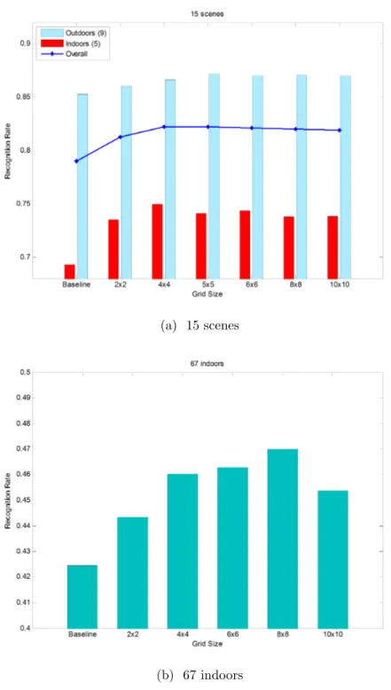
Figure 4.1 shows the recognition rates with different weight matrix(W) sizes. Geometrically partitioning the spatial layout into 5× 5 and 8 × 8 grids yields the best results for the scenes and 67-indoor scenes datasets, respectively. The 15-scenes dataset can be separated into five indoor and nine outdoor categories. We

CHAPTER 4. EXPERIMENTAL SETUP AND RESULTS 28

ignore the industrial category since it contains both indoor and outdoor images. Observe that incorporating spatial information improves the performance rate of the outdoor categories by 2% only. The performance rate for the indoor categories is improved by up to 6%. This difference can be explained by the more orderly form of the descriptors extracted from the indoor images. This improvement is 4.5% for the 67-indoor scenes dataset due to further difficulty and intra-class variations.

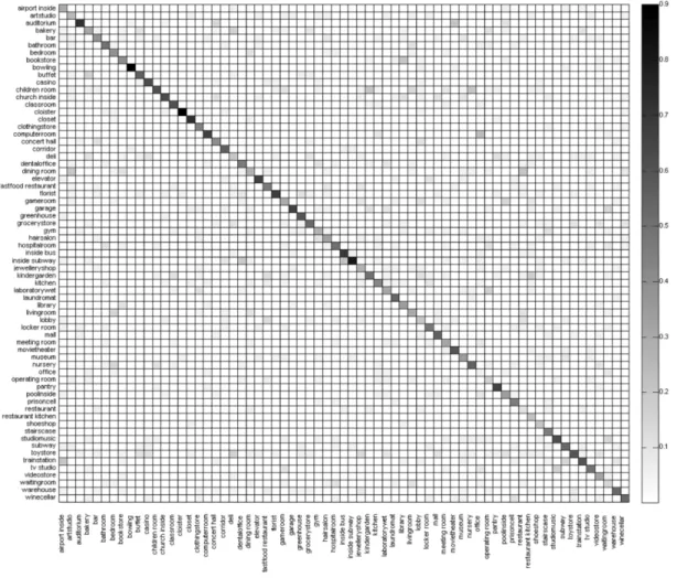
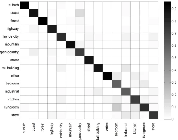
Table 4.2 compares our method with the state-of-the-art scene recognition algorithms. Our method achieves more than 7% improvement over the best pub-lished result in the 67-indoor benchmark [28] and shows competitive performance in the 15-scenes dataset. Figures 4.2 and 4.3 show the confusion matrix for the 67 indoor scenes and 15 scenes datasets, respectively.

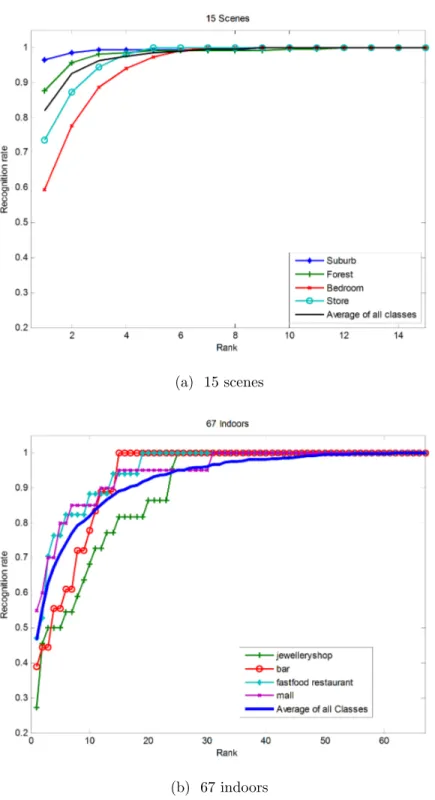
Our method also induces rankings that could naturally be used as a pre-processing step in another recognition algorithm. As shown in Figures 4.4 (a) and (b), our method returns the correct category within the top ten results by ranking the categories for a query image with 82% overall accuracy in the 67-indoor scenes benchmark. This rate is near 100% considering the returned top three results in the 15-scenes dataset (cf. Figure 4.4 (a)). Hence one can utilize this aspect of our algorithm to narrow down category choices, consequently increasing their final recognition rate by analyzing other information channels of the query image with different complementary descriptors or classification methods. Figure 4.5 shows a set of classified images.

CHAPTER 4. EXPERIMENTAL SETUP AND RESULTS 29

(a) 15 scenes

(b) 67 indoors

CHAPTER 4. EXPERIMENTAL SETUP AND RESULTS 30

Figure 4.2: Confusion matrix for the 67-indoor scenes dataset. The horizontal and vertical axes correspond to the true and predicted classes, respectively.

CHAPTER 4. EXPERIMENTAL SETUP AND RESULTS 31

Figure 4.3: Confusion matrix for the 15-scenes dataset. The columns and rows denote the true and predicted classes, respectively.

CHAPTER 4. EXPERIMENTAL SETUP AND RESULTS 32

(a) 15 scenes

(b) 67 indoors

Figure 4.4: Recognition rates based on rankings. Given a query image, if the true category is returned in the top-k results, it is considered a correct classification.

CHAPTER 4. EXPERIMENTAL SETUP AND RESULTS 33

Table 4.3: Recognition Rates for each Category (67-Indoors)

Category Rate Category Rate Category Rate airport inside 0.30 elevator 0.62 movietheater 0.65 artstudio 0.25 fastfood restaurant 0.47 museum 0.35 auditorium 0.72 florist 0.68 nursery 0.70 bakery 0.26 gameroom 0.25 office 0.05 bar 0.44 garage 0.56 operating room 0.16 bathroom 0.50 greenhouse 0.65 pantry 0.65 bedroom 0.38 grocerystore 0.67 poolinside 0.30 bookstore 0.40 gym 0.28 prisoncell 0.40 bowling 0.90 hairsalon 0.38 restaurant 0.10 buffet 0.60 hospitalroom 0.50 restaurant kitchen 0.30 casino 0.63 inside bus 0.74 shoeshop 0.26 children room 0.50 inside subway 0.76 stairscase 0.40 church inside 0.68 jewelleryshop 0.32 studiomusic 0.68 classroom 0.78 kindergarden 0.50 subway 0.48 cloister 0.90 kitchen 0.48 toystore 0.55 closet 0.72 laboratorywet 0.23 trainstation 0.60 clothingstore 0.50 laundromat 0.55 tv studio 0.50 computerroom 0.67 library 0.45 videostore 0.32 concert hall 0.40 livingroom 0.35 waitingroom 0.24 corridor 0.62 lobby 0.25 warehouse 0.52 deli 0.21 locker room 0.43 winecellar 0.48 dentaloffice 0.43 mall 0.45

dining room 0.33 meeting room 0.27

Table 4.4: Recognition Rates for each Category (15-Scenes)

Category Rate Category Rate

suburb 0.96 tallbuilding 0.86 coast 0.88 office 0.95 forest 0.95 bedroom 0.57 highway 0.86 industrial 0.61 insidecity 0.79 kitchen 0.73 mountain 0.92 livingroom 0.80 opencountry 0.72 store 0.77 street 0.88

CHAPTER 4. EXPERIMENTAL SETUP AND RESULTS 34

Figure 4.5: Classified images for a subset of indoor scenes. Images from the first four rows are taken from the 67-indoor scenes and the last two rows are from the indoor categories of the 15-scenes dataset. For every query image the list of ranked categories is shown on the right side. The bold name denotes the true category.

CHAPTER 4. EXPERIMENTAL SETUP AND RESULTS 35

4.4

Evaluation and Results for Auto-annotation

The IAPR dataset we used for evaluation consists of 19875 images. 17665 of these images are used for codebook construction and 1962 images are used for testing purposes. Figure 4.6 displays sample images. For each label, images were obtained having been annotated with it and SIFT descriptors were extracted from patches with bin sizes of 8 and 16 pixels. Then from randomly chosen 100K descriptors a codebook was constructed using K-means consisting of 200 visual words for the particular label. In the testing phase Equation (3.9) was used with different k settings. In both training and testing we scaled the images to have 4:3 aspect ratio (or 3:4 if image height is larger than its width). The performance is measured by calculating the mean precision and recall over all keywords/concepts. The precision of a keyword is defined as the number of images correctly assigned by that word divided by the total number of images assigned by it. Recall of a keyword is defined as the number of images correctly assigned by that word divided by the number of images annotated with that particular word in the ground truth annotation. Table 4.5 shows results with different k settings and Table 4.6 compares our method with a state-of-the-art baseline technique in the auto-annotation literature. Although our method’s performance is inferior there

Figure 4.6: Sample images with respective human annotations from the IAPR dataset.

is much space for improvement. As we mentioned before not all visual words of a category truly describe the concept, hence weighting the visual words with respect to their representative power will likely increase the annotation performance. We also did not take into account the spatial arrangement of the visual words as in the recognition task. Although huge spatial variations of the concepts exist, one

CHAPTER 4. EXPERIMENTAL SETUP AND RESULTS 36

Table 4.5: Annotation performance with different k settings. There are total of 291 concepts.

K= 200 k= 5 k = 10 k = 15 k = 20 k = 25 k = 30 Mean precision 0.07 0.08 0.10 0.11 0.10 0.10

Mean recall 0.05 0.09 0.13 0.17 0.20 0.23 # of words with recall > 0 118 158 194 224 238 252 may still benefit from incorporating the spatial structure especially with concepts that appear in similar schemes/areas in an image. Context modeling for auto-matic image annotation has also attracted attention from the vision community recently. Incorporating the contextual information of the semantic labels has shown to increase the annotation performance [38]. Thus integrating contextual information into the metric function would also enhance annotation accuracy.

Table 4.6: Performance comparison with a state-of-the-art baseline technique NNbMF Makadia et al. [36]

k= 15 k = 5 Mean precision 0.11 0.26 Mean recall 0.13 0.16 # of words with recall> 0 194 199

4.5

Runtime Performance

Compared to learning-based methods such as the popular Support Vector Ma-chines (SVM), the Nearest-Neighbor classifier has a slow classification time, es-pecially when the dataset is too large and the dimension of the feature vectors is too high. Several approximation techniques have been proposed to increase the efficiency of this method, such as [47], and [48]. These techniques involve pre-processing the search space using data structures, such as KD-trees or BD-trees. These trees are hierarchically structured so that only a subset of the data points in the search space is considered for a query point. We utilize the Approximate Nearest Neighbors library (ANN) [47]. For the 67 indoor scenes benchmark, it

CHAPTER 4. EXPERIMENTAL SETUP AND RESULTS 37

takes approximately 0.9 seconds to form a tree structure of a category codebook and about 2.0 seconds to search all query points of an image in a tree structure, using an Intel Centrino Duo 2.2 GHz CPU. Without quantizing, it takes about 100 seconds to search all the query points. For the 15-scenes benchmark, it takes about 1.5 seconds to construct a search tree and 4.0 seconds to search all query points in it. Without quantizing, it takes approximately 200 seconds to search all the query points.

The CUDA implementation of the K-nearest neighbor method [49] further increases the efficiency by parallelizing the search process. We observed ∼0.2 seconds per class needed to search the query points extracted from an image using a NVIDIA Geforce 310M graphics card.

The annotation runtime performance was only tested with the CUDA imple-mentation of the K-NN method. It takes ∼30 seconds to annotate an image.

Chapter 5

Conclusion and Future Work

We proposed a simple, yet effective nearest-neighbor based metric function for recognizing indoor scene images. In addition, given an image our method also induces rankings of categories for a possible pre-processing step for further clas-sification analyses. Our method also incorporates the spatial layout of the visual words formed by clustering the feature space. Experimental results show that the proposed method effectively classifies indoor scene images compared to state-of-the-art methods. We are currently investigating how to further improve the spatial extension part of our method by using other estimation techniques to better capture and model the layout of the formed visual words.

We also employed the proposed metric function for auto-annotation. Although performance of our method is inferior in this domain, we believe that there is much space for improvement. Integrating contextual, spatial information into the metric function will likely improve the annotation accuracy. Also weighting the visual words according to their discriminative power and using complementary features can also enhance the performance.

Bibliography

[1] M. Szummer and R. Picard, “Indoor-outdoor image classification,” in Pro-ceedings of the IEEE International Workshop on Content-Based Access of Image and Video Database, pp. 42–51, January 1998.

[2] A. Torralba, K. Murphy, W. Freeman, and M. Rubin, “Context-based vision system for place and object recognition,” in Proceedings of the IEEE Inter-national Conference on Computer Vision, vol. 1 of ICCV ’03, pp. 273–280, October 2003.

[3] A. Vailaya, A. Jain, and H. J. Zhang, “On image classification: city vs. landscape,” in Proceedings of the IEEE Workshop on Content-Based Access of Image and Video Libraries, pp. 3–8, June 1998.

[4] A. Oliva and A. Torralba, “Modeling the shape of the scene: A holistic representation of the spatial envelope,” International Journal of Computer Vision, vol. 42, pp. 145–175, May 2001.

[5] I. Ulrich and I. Nourbakhsh, “Appearance-based place recognition for topo-logical localization,” in Proceedings of the IEEE International Conference on Robotics and Automation, vol. 2 of ICRA ’00, pp. 1023–1029, 2000.

[6] A. Bosch, A. Zisserman, and X. Muoz, “Scene classification using a hybrid generative/discriminative approach,” IEEE Transactions on Pattern Analy-sis and Machine Intelligence, vol. 30, pp. 712–727, April 2008.

[7] S. Lazebnik, C. Schmid, and J. Ponce, “Beyond bags of features: Spatial pyramid matching for recognizing natural scene categories,” in Proceedings

BIBLIOGRAPHY 40

of the IEEE Computer Society Conference on Computer Vision and Pattern Recognition, vol. 2 of CVPR ’06, pp. 2169–2178, 2006.

[8] S. Se, D. Lowe, and J. Little, “Vision-based mobile robot localization and mapping using scale-invariant features,” in Proceedings of the IEEE Interna-tional Conference on Robotics and Automation, vol. 2 of ICRA ’01, pp. 2051– 2058, 2001.

[9] A. Pronobis, B. Caputo, P. Jensfelt, and H. Christensen, “A discriminative approach to robust visual place recognition,” in Proceedings of the IEEE/RSJ International Conference on Intelligent Robots and Systems, pp. 3829–3836, October 2006.

[10] A. Quattoni and A. Torralba, “Recognizing indoor scenes,” in Proceedings of the IEEE Conference on Computer Vision and Pattern Recognition, CVPR ’09, pp. 413–420, June 2009.

[11] P. Espinace, T. Kollar, A. Soto, and N. Roy, “Indoor scene recognition through object detection,” in Proceedings of the IEEE International Con-ference on Robotics and Automation, ICRA ’10, pp. 1406–1413, May 2010. [12] P. Gehler and S. Nowozin, “On feature combination for multiclass object

classification,” in Proceedings of the IEEE International Conference on Com-puter Vision, ICCV ’09, pp. 221–228, October 2009.

[13] J. Yang, K. Yu, Y. Gong, and T. Huang, “Linear spatial pyramid matching using sparse coding for image classification,” in Proceedings of the IEEE Con-ference on Computer Vision and Pattern Recognition, CVPR ’09, pp. 1794– 1801, June 2009.

[14] J. Wu and J. Rehg, “Beyond the Euclidean distance: Creating effective visual codebooks using the histogram intersection kernel,” in Proceedings of the IEEE 12th International Conference on Computer Vision, ICCV ’09, pp. 630–637, September 29-October 2 2009.

[15] K. Mikolajczyk and C. Schmid, “A performance evaluation of local descrip-tors,” IEEE Transactions on Pattern Analysis and Machine Intelligence, vol. 27, pp. 1615–1630, October 2005.

BIBLIOGRAPHY 41

[16] D. G. Lowe, “Distinctive image features from scale-invariant keypoints,” International Journal of Computer Vision, vol. 60, pp. 91–110, November 2004.

[17] D. Wolpert and W. Macready, “No free lunch theorems for optimization,” IEEE Transactions on Evolutionary Computation, vol. 1, pp. 67–82, April 1997.

[18] O. Boiman, E. Shechtman, and M. Irani, “In defense of nearest-neighbor based image classification,” in Proceedings of the IEEE Conference on Com-puter Vision and Pattern Recognition, CVPR ’08, pp. 1–8, June 2008.

[19] L. Fei-Fei, R. Fergus, and P. Perona, “Learning generative visual models from few training examples: An incremental Bayesian approach tested on 101 object categories,” in Proceedings of the IEEE CVPR Workshop on Generative-Model Based Vision, CVPRW ’04, pp. 178–187, June 2004.

[20] G. Grin, A. Holub, and P. Perona, “Caltech 256 Object Category Dataset,” Tech. Rep. UCB/CSD-04-1366, California Institute of Technology, 2006.

[21] A. Opelt, M. Fussenegger, A. Pinz, and P. Auer, “Weak hypotheses and boosting for generic object detection and recognition,” in Proceedings of the European Conference on Computer Vision, ECCV ’04, pp. 71–84, 2004.

[22] R. Datta, D. Joshi, J. Li, James, and Z. Wang, “Image retrieval: Ideas, influences, and trends of the new age,” ACM Computing Surveys, vol. 40, no. 2), (Article no. 5, 60 pages, 2008.

[23] J. Vogel and B. Schiele, “A semantic typicality measure for natural scene cat-egorization,” in Proceedings of the 26th DAGM Symposium on Pattern Recog-nition Symposium, Lecture Notes in Computer Science, vol. 3175, (T¨ubingen, Germany), pp. 195–203, August 2004.

[24] L. Fei-Fei and P. Perona, “A bayesian hierarchical model for learning natural scene categories,” in Proceedings of the IEEE Computer Society Conference on Computer Vision and Pattern Recognition, vol. 2 of CVPR ’05, pp. 524– 531, June 2005.

BIBLIOGRAPHY 42

[25] P. Quelhas, F. Monay, J.-M. Odobez, D. Gatica-Perez, and T. Tuytelaars, “A thousand words in a scene,” IEEE Transactions on Pattern Analysis and Machine Intelligence, vol. 29, pp. 1575–1589, September 2007.

[26] V. Viitaniemi and J. Laaksonen, “Spatial extensions to bag of visual words,” in Proceedings of the ACM International Conference on Image and Video Retrieval, CIVR ’09, Article no. 37, (New York, NY, USA), pp. 1–8, ACM, 2009.

[27] A. Bosch, X. Mu˜noz, and R. Mart´ı, “Review: Which is the best way to organize/classify images by content?,” Image and Vision Computing, vol. 25, pp. 778–791, June 2007.

[28] N. Morioka and S. Satoh, “Building compact local pairwise codebook with joint feature space clustering,” in Proceedings of the European Conference on Computer Vision, ECCV ’10, pp. 692–705, 2010.

[29] Y. Mori and H. Takahashi, “Image-to-word transformation based on dividing and vector quantizing images with words,” in First International Workshop on Multimedia Intelligent Storage and Retrieval Management, MISRM ’99, 1999.

[30] P. Duygulu, K. Barnard, J. F. G. d. Freitas, and D. A. Forsyth, “Object recognition as machine translation: Learning a lexicon for a fixed image vocabulary,” in Proceedings of the 7th European Conference on Computer Vision, Lecture Notes in Computer Science, vol. 2353, (London, UK), pp. 97– 112, Springer-Verlag, 2002.

[31] J. Shi and J. Malik, “Normalized cuts and image segmentation,” in Pro-ceedings of the IEEE Computer Society Conference on Computer Vision and Pattern Recognition, CVPR ’97, pp. 731–737, June 1997.

[32] J. Jeon, V. Lavrenko, and R. Manmatha, “Automatic image annotation and retrieval using cross-media relevance models,” in Research and Development in Information Retrieval, pp. 119–126, 2003.