Classification of target primitives with sonar using two non-parametric data fusion methods

a г й :-.ΐ; i * Ті-П t·, n r ■:-’'-1 Ѵ?Ш '■'·; \ β /ѵ .-ѵ ; ^■■' ■[ '■j'j^^ ■ ·:\ ^ï‘ S' ■j'* i t ' ^J 'L / .} - 1,J . 'J S- S' ■ Sj J ^

# f k V v : -r·; .·) и -іЦ - \ ^ ;·:· s''ï {Ş V >··. ? r .%· -·>·* Й

w ‘ m^'m- «··■ «-HI 'w·' ‘.^· *' ЧГ·«- W w ■ «** >^' ■ me'm W »' * « i;i м/ V « i ) · W « H, mà Λ -mj »%!/ M i)l 4k

■ГГ^ ··.'·-·· · . *:" «¿C b C; ..· :и ■)>’■«.· Л>, >!j>..i!îiиА »г* : i í, i} . ^ί*Η * · / Λ 4· i ■ .- г·.'^ VJ*, fili Vtó“ V f-'isi 'W·/*, *■, · ’*/.>.*ѵ :^ ’..„• ν’ ^-‘ ·.■..·'^ - .«I ·■- .■ w Φ ^ Ù?

CLASSIFICATION OF TARGET PRIMITIVES WITH

SONAR USING TWO NON-PARAMETRIC DATA

EUSION METHODS

A THESIS

SUBMITTED TO THE DEPARTMENT OF ELECTRICAL AND ELECTRONICS ENGINEERING

AND THE INSTITUTE OF ENGINEERING AND SCIENCES OF BILKENT UNIVERSITY

IN PARTIAL FULFILLMENT OF THE REQUIREMENTS FOR THE DEGREE OF

MASTER OF SCIENCE

By

Birsel Ayriilu

July 1996

I certify that I have read this thesis and that in my opinion it is fully adequate, in scope and in quality, as a thesis for the degree of Master of Science.

Assist. Prof. Dr. Billur Barshan(Supervisor)

I certify that I have read this thesis and that in my opinion it is fully adequate, in scope and in quality, as a thesis for the degree of Master of Science.

r

Assoc. Prof. Dr. Ofner Morgül

I certify that I have read this thesis and that in my opinion it is fully adequate, in scope and in quality, as a thesis for the degree of Master of Science.

Assist. Prof. Dr. Orhan Arikan

Approved for the Institute of Engineering and Sciences:

Prof. Dr. Mehmet B yay

ABSTRACT

CLASSIFICATION OF TARGET PRIMITIVES WITH

SONAR USING TWO NON-PARAMETRIC DATA

FUSION METHODS

Birsel Ayriilu

M.S. in Electrical and Electronics Engineering

Supervisor: Assist. Prof. Dr. Billur Barstian

July 1996

In this study, physical models are used to model reflections from target prim­ itives commordy encountered in a mobile robot’s environment. These tcirgets are differentiated by employing a multi-transducer pulse/echo system which relies on both cimplitude and time-of-flight (TOP) data in the feature fusion process, cillowing more robust differentiation. Target features are generated as being evidentially tied to degrees of belief which are subsequently fused for multiple logical soncirs at different geographical sites. Feature data from multiple logical sensors are fused with Dernpster-Shafer rule of combination to improve the performance of classification by reducing perception uncertainty. Using three sensing nodes, improvement in differentiation is 20% without false decision, however, at the cost of additional computation. Simulation results are verified by experiments with real sonar systems. As an alternative method, neural networks are used for incorporating lecirning of identifying pcirameter relations of target primitives. Amplitude and time-of-flight measurements of .‘]1 sensor pairs cire fused with these neural networks. Improvement in differ­ entiation is 72% with 28% false decision at the cost of elapsed time until the network learns these patterns. These two approaches help to overcome the vul­ nerability of echo amplitude to noise and enable the modeling of non-parametric uncertainty.

Keywords : ultrasonic transducers^ sonar, target classification, sensor-hased robotics, multi-sensor data fusion and integration, non-parametric data fusion, evidential reasoning, belief functions, Dempster-Shafer rmle of combination, logical sensing, artificial neural networks.

ÖZET

HEDEF

SONAR KULLANILARAK

PARAMETRİK OLMAYAN İKİ YÖNTEMLE

SINIFLANDIRILMASI

Birsel Ayrulu

Elektrik ve Elektronik Mühendisliği Bölümü Yüksek Lisans

Tez yöneticisi: Yrd. Doç. Dr. Billur Barsİıan

Temmuz 1996

Bu çcilışıricida, hareketli robot uygulamalarında sıkça karşılaşılan hedef ilkel­ lerinden kaynaklanan yansımaların modellenmesinde fiziksel modeller kul- huııldı. Genlik ve uçuş zamanı verilerine dayanan çok dönüştürücülü dürtii/yankı sistemleri ile hedef ilkelleri tanınmaya çalışıldı. Birden çok mantıksal sonar için atanan inanç değerleri taşıyan hedef özellikleri sürekli olarak birleştirildi. Algı belirsizliklerini azaltıp smıilandırma başarısını arttırm ak için yapılan bu birleştirme işlemi için Dempster-Shafer birleşim ku­ ralı kullanıldı. Uç algılayıcı çifti kullanılarak sınıflandırma işleminde fazladan yapıları işlemlere kcirşm %20 ye varan bir başarım artışı elde edildi. İkinci bir yöntem olarak, tanıtım parametre yakınlıklarınm beraberce öğrenilmesi için yapay sinir ağları kullanıldı. Bu ağ yapısında devrenin bu hedef ilkel­ lerini öğreninceye kadar geçen zaman ve 31 algılayıcı çiftine rağmen genlik ve uçuş zarricinı ölçümleri kullanılarak sınıflandırma işleminde %72 ye varan bir başarı ve %28 yanlış karar elde edildi. Bu çalışmada kullanılan iki yöntemin lıer biri yankı genliğinin gürültüye kcirşı olan duyarlılığının üstesinden gelm­ eye yardımcı olduğu gibi pararnetrik olmayan belirsizliklerin modellenrnesini de sağhımaktadır.

Anahtar Kelimeler : sesötesi duyucular, engel sınıflandırma, robotik algılama, pararnetrik olmayan veri tümleşimi, Dempster-Shafer birleşim kuralı, mantıksal algılama, yapay sinir ağları.

ACKNOWLEDGMENTS

I would like to thank everyone who contributed to this thesis. First of all, 1 would like to tluink Dr. Billur Bcirshan for her supervision, guidance, suggestions and encouragement throughout the development of this thesis.

I would like to thank Dr. Aydan M. Erkinen, Dr. ismet Erkmen and Dr. Ömer Morgül for their helpful suggestions.

Many thanks to Aykut Erdem for his help and encouragement.

Many thanks also to Gül Aydın, Nur Kurt, Fatma Çalışkan and Lütfiye Durak for their help.

T A B L E OF C O N T E N T S

1 INTRODUCTION 1

2 SONAR SENSING AND TARGET DIFFERENTIATION

ALGORITHM 5

2.1 Physical Reflection Models of Sonar from Different Target Prim­ itives ... .5 2.2 Target Differentiation Algorithm ... 8

3 LOGICAL SENSING AND FEATURE FUSION OF MULTI­

PLE SENSOR PAIRS 15

3.1 Logical S e n s in g ... 1.5 3.1.1 Feature Fusion from Multiple Sonars for Plane-Corner

Id e n tific a tio n ... 16 3.1.2 Fusion of Range and Azimuth E s tim a te s ... 18 3.1.3 Inclusion of Acute Corner Tcirget Type in the Classifica­

tion P ro c e s s ... 22 3.2 Sirnulcition R e s u l t s ... 24 3.2.1 Feature Fusion for Plane-Corner IdentifiCcition... 24 3.2.2 Simulation Results of Fusion of Range and Azimuth Es­

timates ... 28 3.2.3 Simuhition Results with Acute Corner Tcirget Model 31

4 VERIFICATION WITH EXPERIMENTAL DATA 41

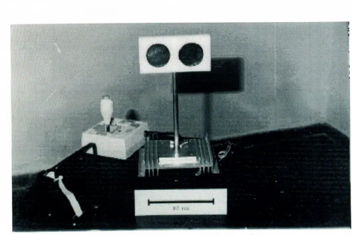
4.1 Experimental S e t - u p ... 41

4.2 Experirnentcü Results with Polaroid T ransducers... 42

4.3 Experimental Results with Panasonic T rausducers... -52

5 DIFFERENTIATION OF TARGET PRIMITIVES WITH ARTIFICIAL NEURAL NETWORKS 85 5.1 Introduction to Artificial Neurcil N e tw o rk s ... 85

5.2 Target Classification with Artificial Neural Networks 87 6 CONCLUSION 106 6.1 D iscussion... 106

6.2 Conclusion... 107

A GEOMETRIC TARGET AND ECHO SIGNAL MODELS 108 A.l Plcxiicir Target M o d e l... 108

A.2 Corner Target M o d e l... 110

A.3 Edge Target M o d e l... 112

A.4 Cylinder Target M o d e l...113

A.5 Acute Corner M o d e l ...116

A.6 Effect of Transducer Separation and Range on TOE and Ampli­ tude C haracteristics...124

B CHOICE OF NOISE MULTIPLICITY FACTOR k IN THE CLASSIFICATION ALGORITHM 130

D AMPLITUDE CHARACTERISTICS OF EDGES AND

CYLINDERS 137

E RELATIONSHIP BETWEEN AND at

E. 1 Relation betwoien <ta and at in a Typical Sonar Echo

E.2 Relationship between a^. and at in a Linecir Signal Model

140

. 140 . 145

LIST OF F IG U R E S

2.1 A typical echo of the ultrasound ranging system... 6 2.2 Sensitivity region of an ultrasonic transducer pair... 7 2.3 Configuration of the trcinsducer pair with respect to a point target. 7 2.4 Target primitives modeled cuid differentiated in this study. . . . 8 2.5 The TOF characteristics of targets when the target is at r = 2

m (a) phme (b) corner (c) edge with 6 ^ = 90° (d) cylinder with

i'c = 20 cm. 9

2.6 TOF characteristics of acute corner at r = 2 m with (a) Oc = 30° (b) 0, = 45° (c) 0c = 60° (d) 0c = 90°. 10 2.7 Amplitude characteristics when the targets are at r — 2 m(a)

plcine (b) corner (c) edge with 0e — 90° (d) cylinder with Vc — 20 cm... 13

3.1 Common coordinate system for n pairs of sonar sensors... 19 3.2 Projected range and azimuth for transducer pair i. 19 3.3 Position of a plane with respect to each sensor pciir... 21 3.4 Belief assignment for a single transducer pciir. 25 3.5 Classification with a single transducer pair... 26 3.6 Chissification and data fusion with three transducer pairs. 26 3.7 Clcissilication with a single transducer pair without the (ta term

3.8 Improvement in the probability of correct classification caused by data fusion with three transducer pairs... 27 3.9 Projected range and azimuth estimates at <;^ = 90° for the sen­

sor pair which is located at (a),(b) (—0.5.1.0) (c),(d) (—2.0,2.0) (e),(f) (2.0,2.0) (g),(h) Fused range and azimuth estimates. . . . 29 3.10 Projected range and azimuth estimates at = 135° for the sen­

sor pair which is located at (a),(b) (—0.5.1.0) (c),(d) (—2.0,2.0) (e),(f) (2.0,2.0) (g),(h) Fused range and azimuth estimates. . . . 30 3.11 Position of the transducer pair and acute corner... 31 3.12 Assignment of beliefs by a transducer pair when an acute corner

of 6 c = 30° at r — 2 m is scanned for noise standard deviation values (a) a a — 0.0 (b) aA = 0.002 (c) cr^ = 0.003. ... 32

3.13 Assignment of beliefs by a transducer pair when cui acute corner at r — 2 m with 6 c ■ 45° is scanned for noise standard deviation values (a) cta — 0.0 (b) (Ta = 0.002 (c) <7a = 0.003... 33 3.14 Assignment of beliefs by a transducer pair when an cicute corner

cit ?’ = 2 rn with 6 c = 60° is scanned for noise standard deviation Vcilues (a) (Ja = 0.0 (b) = 0.002 (c) cta = 0.003... 34

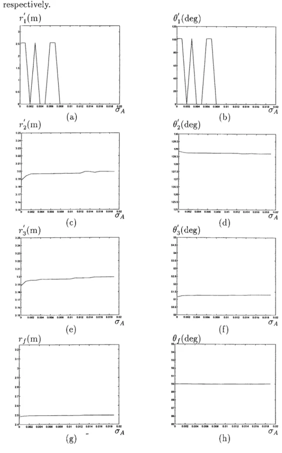
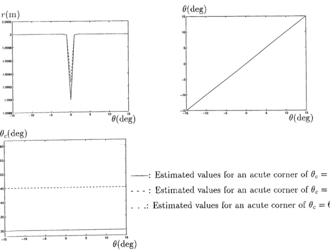
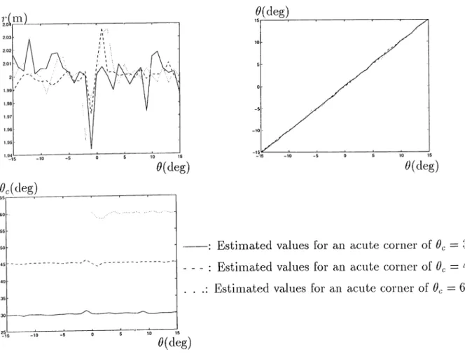
3.15 Estinuited values of range r, inclination angle 6 , and angle of acute corner 6 c, without noise for acute corners of 6 c = 30°, 45° and 60°... 35 3.16 Estimated values of range r, inclination angle 6 , and angle of

acute corner 6 c, with cta = 0.002 for acute corners of 6 c ~

30°, 45° and 60°... 36

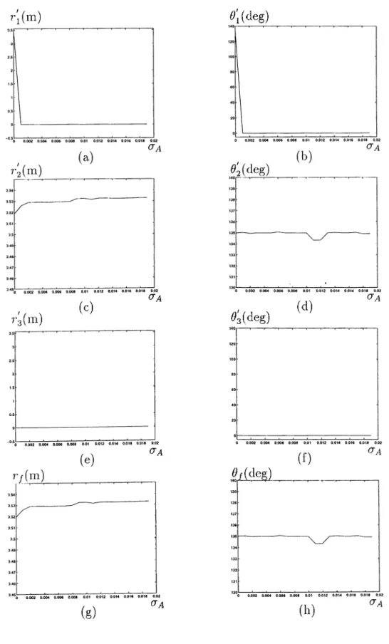
3.17 Estimated values of range inclination angle 6 , and angle of acute corner 6 c, with aA = 0.003 for acute corners of 6 c — 30°, 45° and 60°... 37 3.18 Classification results with a single transducer pair by the second

approach when an acute corner at r = 2 in is scanned with (a) 6 c = 30° (b) il, = 45° (c) = 60°... 39

3.19 The classification result for the acute corner of &c = 60" when

at and aji terms are replaced with zero in the corresponding

cilgorithms. 39

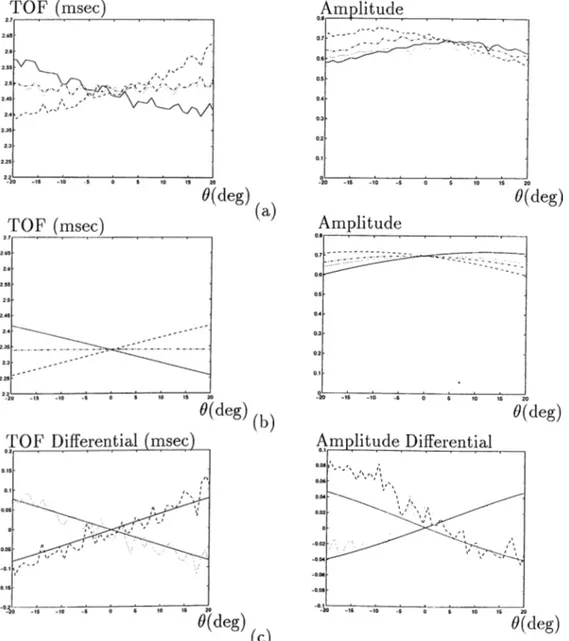
4.1 Comparison of TOF chcii’cicteristics of a phme and the theoretical predictions when a Polaroid transducer pair with separation d = 15 cm is employed at r = 80 cm (a) experimental results (b) theoretical results (c) differential T O F... 43 4.2 Configuration of Polaroid transducer pair in the real system. . . 44 4.3 Differentials in TOF characteristics of a plane when a Polaroid

ti'cinsducer pair with separation d = 15 cm is employed at the range values (a) r =30 cm (b) r =50 cm (c) r =70 cm (d) r =90 cm (e) r =110 cm (f) r =130 cm... 45 4.4 Comparison of TOF and amplitude characteristics of a cylinder

of ?’c = 7.5 cm with the theoretical predictions when a Polaroid transducer pair with separation d = 15 cm is employed at r = 80 cm (a) experimental results (b) theoretical results (c) differenticd signals... 46 4.5 Differentials in TOF and amplitude characteristics cylinder with

rj'c - 7.5 cm when a Polaroid transducer pair with separation

d = 15 cm is employed at the range values (a),(b) r =50 cm (c),(d) r =70 cm (e),(f) r =90 cm (g),(h) r =110 cm. ... 47 4.6 Comparison of TOF and amplitude characteristics of a cylinder

of Vc — 5.0 cm with the theoretical predictions when a Polaroid transducer pair with separation d = 15 cm is employed at r = 80 cm (a) experimental results (b) theoretical results (c) differential sigricils... 48 4.7 Differentials in TOF and amplitude characteristics of a cylinder

with I'c — 5.0 cm when a Pohiroid transducer pair with separa­ tion d = 15 cm is employed at the range values (a),(b) r =50 cm (c),(d) r =70 cm (e),(f) r =90 cm (g),(h) r =110 cm... 49

4.8 Comparison of TOF and amplitude characteristics of a cylinder of 7’c = 2.5 cm with the theoretical predictions when a Polaroid trcuisducer pair with separation d = 15 cm is emplo3^ed at r = 80

cm (a) experimental results (b) theoretical results (c) differential signals... 50 4.9 Differentials in TOF and cimplitude chariicteristics of a cylinder

with Tc = 2.5 cm when a Polaroid transducer pair with separa­ tion d = 15 cm is errp^loyed at the range values (a),(b) r =50 cm (c),(d) r =70 cm (e),(f)r =90 cm (g),(h) r =110 cm. 51 4.10 Configurcition of the Pcinasonic transducer pair in the real system. 53 4.11 Cross-section of the Panasonic transducer... 54 4.12 Comparison of TOF and amplitude characteristics of a phme

with the theoretical predictions when a Panasonic transducer pair with separation d = 24 cm is employed at r = 50 cm (a) experimental results (b) theoretical results (c) differential sigiicds. 56 4.13 Differentials in TOF and amplitude characteristics of a plane

when a Panasonic transducer pair with separation d = 24 cm is employed at the range values (a),(b) r =20 cm (c),(d) r =30 cm

(e),(f) r =40 cm (g),(h) r =50 cm. 57

4.14 Differentials in TOF cind amplitude chciracteristics of a plane when a Panasonic transducer pair with separation d = 24 cm is employed at the range values (a),(b) r =60 cm (c),(d) r =80 cm (e),(f) r =100 cm (g),(h) r =120 cm... 58 4.15 Comparison of TOF and amplitude charcicteristics of a corner

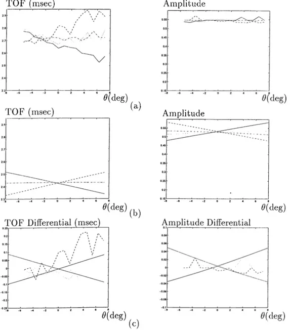
with the theoretical predictions when a Panasonic ti’cinsducer pair with separation d = 24 cm is employed cit r = 40 cm (a) experimental results (b) theoretical results (c) differenticil sigiicils. 59 4.16 Differentials in TOF and amplitude chciracteristics of a corner

when a Panasonic transducer pair with separation d — 24 cm is employed at the range values (a),(b) r =40 cm (c),(d) r =60 cm

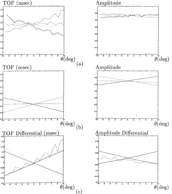
4.17 Comparison of TOF and amplitude characteristics of an acute corner of Oc = 60° with the theoretical predictions when a Pana­ sonic transducer pair with separation d = 24 cm is employed at

r = 40 cm (a) experimental results (b) theoretical results (c)

differential signals.

4.18 Differentials in TOF and amplitude characteristics of an acute corner of 0c - 60° when a Panasonic transducer pair with sepa­ ration d = 24 cm is emi^loyed at the range values (a),(b) r — 40 cm (c),(d) r = 60 cm (e),(f) r = 80 cm (g),(h) r = 100 cm. . . 4.19 Comparison of TOF and amplitude characteristics of a cylinder of 7'c = 7.5 cm with the theoi’etical predictions when a Panasonic transducer pciir with separation d — 24 cm is employed at r = 20 cm (a) exiDerimental results (b) theoreticcd results (c) differentiell signals... ... 4.20 Differentials in TOF and amplitude characteristics of cV cylinder

with 'I'c — 7.5 cm when a Panasonic transducer pair with sepci- ration d = 24 cm is employed at the riinge values (a),(b) r = 20 cm (c),(d) r = 40 cm (e),(f) r = 60 cm (g),(h) r = 80 cm. . . . 4.21 Comparison of TOF and amplitude characteristics of a cylinder

of Tc = 5.0 cm with the theoretical predictions when a Panasonic transducer pair with separation d = 24 cm is employed at r = 40 cm (a) experimental results (b) theoretical results (c) differential

61

62

63

64

SI 65

4.22 Differentials in TOF and amplitude characteristics of a cylinder with ry = 5.0 cm when a Panasonic transducer pciir with sepa­ ration d = 24 cm is employed at the range values (a),(b) ?· = 20 cm (c),(d) = 40 cm (e),(f) r == 60 cm (g),(h) r = 80 cm. . . . 66 4.23 Cornpcirison of TOF and amplitude characteristics of a cylinder

of Vc — 2.5 cm with the theoretical predictions when a Panasonic transducer pair with separation d = 24 cm is employed at ?’ = 40 cm (a) experimental results (b) theoretical results (c) differential signals... 67

4.24 Differentials in TOF and amplitude characteristics of a cylinder with '/’c = 2.5 cm when a Panasonic transducer pair with sepa­ ration d = 24 cm is employed at the range vcilues (a),(b) r =40 cm (c),(d) r =60 cm... 68 4.25 Comparison of TOF and amplitude characteristics of a cylinder

of ?’c = 7.5 cm with the theoretical predictions when a Panasonic transducer pair with separation d = 8 cm is employed at r = 40 cm (a) experimental results (b) theoretical results (c) differential signals... 69 4.26 Differentials in TOF and amplitude characteristics of a cylinder

with Vc = 7.5 cm when a Panasonic transducer pciir with sepa­ ration d = 8 cm is employed at the range values (a),(b) r = 20 cm (c),(d) r = 40 cm (e),(f) r = 60 cm... 70 4.27 Differentials in TOF and cirnplitude characteristics of a cylinder

with 7'c — 7.5 cm when a Pcumsonic transducer pair with sepci- ration d = 8 cm is employed at the range values (a),(b) r = 80 cm (c),(d) r = 100 cm (e),(f) r = 120 cm... 71 4.28 Comparison of TOF and amplitude characteristics of a cylinder

of Vc = 5.0 cm with the theoretical predictions when a Panasonic trcvnsducer pair with separation d = 8 cm is employed at ?■ = 40 cm (a) experimental results (b) theoretical results (c) differential signals... 72 4.29 Diflerenticds in TOF and amplitude characteristics of a cylinder

with '/y = 5.0 cm when a Panasonic transducer pair with sepa­ ration d = 8 cm is employed at the range values (a),(b) r = 20 cm (c),(d) r = 40 cm (e),(f) r = 60 cm (g),(h) = 80 cm... 73 4.30 Comparison of TOF and amplitude characteristics of a cylinder

of = 2.5 cm with the theoretical predictions when a Panasonic transducer pair with separation d = 8 cm is employed at r = 20 cm (a) experimental results (b) theoretical results (c) differential signals... 74 4.31 Differenticils in TOF and amplitude characteristics of a cylinder

with Tc = 2.5 cm when a Pcinasonic trcinsducer pair with sepa- riition d = 8 cm is employed at the range values (a),(b) v — 20 cm (c),(d) r = 40 cm (e),(f) r = 60 cm (g),(h) r = 80 cm... 75

4.32 Comparison of TOF and amplitude charcicteristics of a cylinder of 7’c ■ 1.5 cm with the theoretical predictions when a Paiicisonic transducer pair with separation d = 8 cm is employed at r = 40 cm (a) experimental results (b) theoretical results (c) differential signals... 76 4.33 Differentials in TOF and amplitude characteristics of a, cylinder

with Tc = 1.5 cm when a Panasonic transducer pair with sep¿i- ration d = 8 cm is employed at the range values (a),(b) r = 20 cm (c),(d) r = 40 cm (e),(f) r = 20 cm (g),(h) r = 40 cm... 77 4.34 Belief assignment to a plane at r — 50 cm scanned with a, Pana­

sonic triinsducer pair with separiition d = 24 cm... 79 4.35 Estimated (a) range and (b) azimuth values of a plane at r = 50

cm scanned with a Panasonic transducer pair with sel^aration d = 24 cm... 79 4.36 Belief assignment to a corner cit r = 80 cm which is scanned

with Pciiicisonic transducers with separation d = 24 cm... 80 4.37 Estimated (a) range (b) azimuth and (c) wedge angle of a corner

at r = 80 cm scanned with Panasonic transducers with separa­ tion d - 24 cm... ... 80 4.38 Belief assignment to an acute corner of = OO'' at r = 40

cm scanned with a Paucisonic transducer pair with separation d = 24 cm... 81 4.39 Estimated (a) range (b) azimuth ¿ind (c) angle of an cicute corner

of Oc — 60° at r — 40 cm scanned with a Panasonic trcinsducer pair with separation d = 24 cm... 81 4.40 Rcinge readings of the transducer pair when located at

(—0.21,0.17) in a rectangular room... 83 4.41 Belief assignment for the sensors located at (a) (0.0,0.0) (b)

(-0.21,0.17) (g-) (0.35,0.29). 83

4.42 Pairwise fused beliefs for the Panasonic transducers located at (a) (0.0,0.0) and (-0.21,0.17) (b) (0.0,0.0) and (0.35,0.29) (c) (—0.21,0.17) and (0.35,0.29) (d) Results when the decision of all three pairs are fused... 84

5.1 The two most common choices for the activation function; (a) sigmoid (b) hyperbolic tangent functions... 86 5.2 Structure of the neural network used in this study... 89 5..‘1 Percentage of success of the neural network which is trained with

the i:>atterns at r = 0.5 m for (a) plane (b) corner (c) edge of dg = 90“ (d) cylinder of iy = 15 cm (e) acute corner of dg = 60“ (f) acute corner of dg = 45“ (g) acute corner of dg = 30“ (h)

ovei'cdl success of this network. 94

5.4 Percentage of success of the neural network which is triiined with the patterns at r — 0.5 m for all target primitives at (a) r - 0.5 rn (b) r = 1.0 m (c) r = 1.5 m (d) r = 2.0 rn (e) r = 2.5 m (f)

overall success of this network. 95

5.5 Percentcxge of success of the neural network which is trained with the patterns at r = 1.0 m for (a) plane (b) corner (c) edge of dg = 90“ (cl) cylinder of rg = 15 cm (e) acute corner of dg = 60“ (f) cicute corner of dg = 45“ (g) acute corner of dg = 30“ (h)

overall success of this network. 96

5.6 Percentage of success of the neural network which is trained with the patterns at ?" = 1.0 m for all target primitives at (a) r = 0.5 m (b) r = 1.0 m (c) r = 1.5 m (cl) r = 2.0 m (e) r = 2.5 m (f)

overall success of this network. 97

5.7 Percentage of success of the neural network which is trained with the patterns at r = 1.5 m for (a) plane (b) corner (c) edge of dg = 90“ (cl) cylinder of ?y = 15 cm (e) acute corner of dg = 60“ (f) acute corner of dg = 45“ (g) acute corner of dg — 30“ (h)

ovcii'cill success of this network. 98

5.8 Percentage of success of the neural network which is learned with the patterns at r = 1.5 m for all target primitives at (a) r = 0.5 m (b) r = 1.0 m (c) r = 1.5 m (cl) r = 2.0 m (e) r = 2.5 m (f)

5.9 Percentage of success of the neural network which is trained with the patterns at r = 2.0 m for (a) plane (b) corner (c) edge of

Oc = 90^' (d) cylinder of iy = 15 cm (e) acute corner of Oc = 60*^

(f) acute corner of Oc = 45° (g) acute corner of Oc = -30° (h) overall success of this network...100 5.10 Percentage of success of the neural network which is trained with

the patterns at r = 2.0 m lor all target primitives at (a) ?■ = 0.5 m (b) r = 1.0 m (c) r — 1.5 m (d) ?■ = 2.0 rn (e) ?’ = 2.5 rn (f) overall success of this network...101 5.11 Percentage of success of the neural network which is trained with

the patterns at r = 2.5 rn for (a) phine (b) corner (c) edge of

9e = 90° (d) cylinder of Vc = 15 cm (e) acute corner of Oc = 60°

(f) acute corner of Oc = 45° (g) acute corner of Oc = 30° (h) overall success of this network... 102 5.12 Percentage of success of the neural network which is trained with

the patterns at r = 2.5 m for cill target primitives at (a) r = 0.5 m (b) r = 1.0 m (c) r = 1.5 in (d) r = 2.0 m (e) r = 2.5 m (f) overall success of this network...103 5.13 Percentage of success of the neural network which is trained with

the patterns at r = 0.5,1.0,1.5,2.0 and 2.5 m for (a) plane (b) corner (c) edge of Oe = 90° (d) cylinder of ry = 15 cm (e) acute corner of Oc = 60° (f) acute corner of Oc = 45° (g) acute corner of Oc - 30° (h) overall success of this network... 104 5.14 Percentage of success of the neural network which is trained

with the patterns at r = 0.5,1.0,1.5,2.0 and 2.5 m for all target primitives at (ci.) r = 0.5 in (b) r = 1.0 m (c) r = 1.5 m (d)

r = 2.0 m (e) r -- 2.5 m (f) overall success of this network. . . . 105

A.l Geometry of the problem with the given sensor pair when the target is a plane... 108 A.2 Geometry of the problem when the target is a corner... 110 A.3 Geometry of the problem when each surface reflects specularly. . I l l A.4 Geometry of the problem when the target is an edge... 112

A.5 Geometry of the problem when the target is a cylinder with radius i'c... 113 A.6 Amplitude curves of the detected signal in the case of (a) plaricu·

target (b) cylindrical target with radius 10 m ... 115 A.7 Geometry of the problem when the target is an acute corner. . . 116 A.8 Geometry of the problem when the tcirget is an acute corner and

0 ^ \0 \ — Oo, ^1 + ^o]...117 A.9 Geometry of the problem when the tcirget is an acute corner

with critical angle O2 ...117 A. 10 Geometry of the problem when each surface of acute corner is

considered a specular reflector when 0 ^ [61 — 0 o,0 2 )... 119 A. 11 Geometry of the problem when each surface of acute corner is

considered a specular reflector and 0 6 [—0 2 ·, ^2]· (a) 0 € {—0 2 , 0), (b) 0£{O ,02Í {c) 0 ^ Q ° ...123

A. 12 A planar target falls (a) within the intersection of the sensitivity pcitterns of both transducers (b) outside the intersection of the sensitivity patterns so thcit cross signals are not detected... 126 A. 13 TOF and amplitude differentials versus trcuisducer separation at

various I'cinge values for (a)-(b) plane (c)-(d) corner (e)-(f) edge of 0e — 90" (g)-(h) cylinder of = 15 cm... 128 A. 14 Maximum TOF and cimplitude differentials versus transducer

separation at various range values for cicute corners of (a)-(b)

0, = 60" (c)-(d) 0, = 45" (e)-(f) 0, = 30"... 129

B. l Noisy amplitude for a plane at ?■ = 2 rii with noise standard deviation (a) = 0 (b) aA = 0.005 (c) (Ta = 0.01 (d) aA = 0.03

(e) (7^ = 0.05 (f) (T^ = 0.1...131

B.2 Noisy amplitude for a plane at ?’ = 2 in with noise standard deviation (a) cta = 0 (b) cta = 0.001 (c) aA = 0.002 (d) d/i = 0.003 (e) (7^ =J).004 (f) (7^ = 0.005... 132 B.3 Classification results of one transducer pair when kA = 0...133

в .4 Classification results for multiples of noise stanclcird deviation,

ал, with (a) кл = 0.5 (b) — 1.0 (c) k^ = 1.5 (d) k^ = 2.0 (e)

кл = 3.0 (f) кл = 4.0... 134

D.l Amplitude characteristics of an edge with (a) 0^ = 30" (b) 0^ = 45" (c) 0^ = 60" (cl) = 75" (e) = 90"...138 D. 2 Amplitude characteristics of a cylinder with (a) Гс = 5 cm

(b) '/’c = 20 cm (c) Гс = 40 cm (d) Гс = 80 cm (e) r,, = 1 m (f) r, = 10 m ...139

K.l A typical echo waveform... 141 E. 2 StandcU’d deviation and mecin of TOF estimate over 1000

reiil-izations when a typical echo waveform is used with (a) r = 0.005 (b) T = 5сгл (c) r = пал and cr,4 = 0.005... 143

E.3 True values (left column) ¿uid bias (right column) in the TOF measurements over 1000 realizations when a typical echo wave­ form is used with (a) r = 0.005 (b) r = 5сгд (c) r = пал and (ТЛ = 0.005... 144 E.4 A typiccil echo waveform and threshold level r ...145 E.5 Standard deviation and mean of ТОБ' estimate over 1000 real­

izations when cl linear signal model of form y{t) = at is used with (a) r = 0.005 (b) r = (c) r = псга and (Xa — 0.01. . . 146 l'h6 True value (left column) and bias (right column) in the TOF

measurements over 1000 realizations when a linear signal model of form y(t) = at is used with (a) r = 0.005 (b) r = 5aA (c) r = 7i<7a and (7a = 0.01...147

E.7 Standard deviation and mean of TOF estimate over 1000 real­ izations when a linear signal model of form y(t) — lOOZ is used with (a) r = 0.005 (b) r = 5cr^ (c) r = mcr^ and = 0.01. . . 148 E.8 True value (left column) and bias (right column) in the TOF

rneasLirciments over 1000 realizations when a linear signal model of form y(t) — lOOi is used with (a) r = 0.005 (b) r = 5aA (c) r = ncTA and = 0.01...149

E.9 Standard deviation and mean of TOF estimate over 1000 real­ izations when a linear signal model of form y{t) = 1000/ is used with (a) r = 0.005 (b) r = 5cr^ (c) r = hcta and a a = 0.01. . . 150 E.IO True value (left column) and bias (right coluimi) in the TOF

rnecisurernents over 1000 realizations when a linecir signal model of form y(t) = 1000/ is used with (a) r = 0.005 (b) r = 6 aa (c) r = naA and = 0.01...151

LIST OF T A BLES

3.1 Plane/corner differentiation by Dempster-Shcifer rule of combi-iicition... 17 3.2 Target differentiation by Dernpster-Shafer rule of combination. . 23 3.3 Relcitionship between cr^ and at... . . .■... 32 3.4 Maximum differences between TO F’s for acute corners for three

vcilues oi Oc... 37 4.1 Minimum cind mciximum range values at which chita can be col­

lected for the target primitives. .32

•5.1 Nundser of learning cycles and the avercige error for the network which is trained with the patterns at range r. 88 5.2 Desired output patterns of the designed neural network... 90 5.3 Success of recognition at different ranges of the neurcd network

which is trcdned with the pcitterns at r - 0.5 m ... 90 5.4 Success of recognition at different riinges of the neurcd network

which is trained with the patterns at ?’ = 1.0 rn... 91 5.5 Success of recognition at different ranges of the neural network

which is trained with the patterns at r = 1.5 m ... 91 5.6 Success of recognition at different ranges of the neural network

which is trainecTwith the patterns at r = 2.0 m ... 91 5.7 Success of recognition at different ranges of the neural network

5.8 Success of recognition cit different ranges of the neural network which is trained with the patterns at r = 0.5, f.0 ,1.5,2.0 and 2.5 in... 93 A.l The fixed inclination angle 6 for all target primitives... 124 A.2 The critical d/r values for edge and cylindrical target primitives. 127

C hapter 1

IN T R O D U C T IO N

There is no single sensor which perfectly detects, locates and identifies targets under all circumstances. Although some sensors are more accurate at locating and tracking objects, they do not provide identity information or vice versa. This points to the need for combining data from multiple sensors via data fusion techniques. The primary aim of the data fusion is to combine data, from multiple sensors to perform inferences that may not be possible from a single sensor. Data fusion applications span a wide domain including automatic target recognition, mobile robot navigation, target tracking, ciircra.ft navigation and military applications [1, 2]. In robotics a.pplications, data fusion enables intelligent sensors to be incorporated into overall operation of a robot so that they can interact with and operate in an unstructured environment without tlie conq^lete control of a. human operator [3].

Qualitcitive benefits which are gained through multisensor data fusion in­ clude improved operational performance, extended spaticd coverage, reduced ambiguity of inferences, improved detection, improved system reliability and enhanced spatial resolution. Quantitatively, the benefit of multisensor data fusion is the improvement of the accuracy of inferences such as estimation of location or identity declaration.

Data fusion can be accomplished by using geometrically, geographically or physiccilly different sensors at different levels of representation such as signal- level, pixel-level, feature-level and symbol-level fusion. In this study, we use |)hysically identical sonar sensors to combine intbrmation when they are located at geographiccilly different sensing sites. Feature-level fusion will be used to provide a system performing an object recognition task with additional features

Problems associated with multisensor data fusion center around the m eth­ ods used for modeling the error or uncertainty in sensory information, data fusion process and operation of the overall system. There are т а л у frame­ works tor multisensor data fusion. In this study two of them are used: The first one is the Dempster-Shafer evidence processing which is used in the data fusion at the level of evidence. Second one is artificial neural networks which provide a fairly well-established formalism with which to model the multisensor fusion process.

that can be used to increase its recognition capabilities.

One mode of sensing which is potentially very useful cuid cost-effective lor mobile robot applications is sonar. Since acoustic sensors are light, ro­ bust and inexpensive devices, they are widely used in applications such as navigation of autonomous vehicles through unstructured environments [4, 5], map-building [6, 7], target-tracking [8] and obstcicle avoidcince [9]. Although there are difficulties in the interpretation of sonar data due to multiple specuhir reflections, poor angular resolution of soruir and establishing correspondence between multiple echoes on different receivers [10], these difficulties can be overcome by employing accurate physical models for the reflection of soiicu·. d'he most popular sonar rcinging system is based on the time-of-flight (TOF) measurement which is the time elapsed between the trcinsmission of a pulse and its reception [11]. Since the amplitude of sonar sigmils is very prone to environ­ mental conditions and since standard electronics for the Polaroid sensor [12] does not provide the echo amplitude directly, most sonar systems exploit only TOF inlbrmation. However, for better chissification of some common target primitives, multi-transducer pulse/echo systems can be employed which rely on both cunplitude and TOF infbrmation to differentiate these targets. In ear­ lier work by Barshan and Kuc, both TOF and amplitude of the echo signal is used to differentiate planes and corners using a statistical error model for the noisy signals [13]. Here we extend this work to develop algorithms which cover additional target types and data fusion techniques. Differential models of planes, edges, corners and cylinders hcive also been used by other researchers in target trcxcking applications [14]. In most navigation systems including sonar, two-dimensional sensing models are employed where it is assumed that tar­ gets extend into the third dimension with the Sciine horizontal cross-section. However, it is not the case that the tcirgets are in the same horizontal plane of the sensor in general. This problem has been handled by some researchers by providing the sensor with the flexibility to track 3-D targets which are not necessarily in the same horizontal plane as the sensor [15, 16, 17].

Sensoi'y information from a single sonar has poor angulcir resolution and is not sufficient to differentiate some target primitives such as phuie and cor­ ner [13]. Many researchers employ multiple sensor configurations in their ap­ plication which Ccin be of the same type, or of different t}^pes complernentciry in nature. Flynn proposed a model for combining the information from sonar and infrared sensors to build more accurate maps of the environment, in particular door edges, where sonar may fail due to its low resolution [18]. Durrant-Whyte modeled information obtained from multiple sensors to deal effectively with cooperative, competitive, and complementary interactions between various in­ formation sources [19]. A neural network model is proposed for sensory fusion based on the target localization system of the barn owl [20]. To overcome the problems that origimite from the difficulties in the interpretation of sonar data Ibr cicoustic imaging, ci system which combines acoustic hologrciphy with mul­ tilayer feedforward neui'cil networks for 3-D object recognition is proposed in [21]. Neural networks are also used in sonar appliccitions [22] and-identification of ships from observed parametric radar data [23]. A comparison between neu­ ral networks cuid standard classifiers for radar-specific emitter identification is provided by Willson [24].

The objective in this thesis is to fuse information from uncertain envi­ ronmental data acquired by multiple sonars at distinct geographical locations for strategic target recognition using two non-pararnetric methods. First, the ultrasonic reflection process from commonly encountered target primitives is modeled such that soncir pairs became evidential logiccd sensors. Logical sen­ sors, as opposed to physiccil sensors that acquire real data, process real sensory data in order to generate perception units which are context-dependent inter- [iretations of the real data [25]. By processing the real data, logical sensors classify the tcirget primitives which are limited to plane, corner and cicute corner initially. An automated perception system for mobile robots fusing uncertain sensory information must be reliable in the sense that it is predictable. There­ fore quantitative cxpprocxches to uncertainty are needed. These considerations favor measure-based methods handling sensory data (both physical and logical) at different levels of granularity related to the resolution of the data cxs well as the time constants of the different sensors. This desire motivates our attem pt to abstract the sensor integration problem in a conceptual model where un­ certainty about evidence' and knowledge can be measured and systematically leduced. To overcome the vulnerability of echo amplitude to noise, multiple sensors are used in the decision making, and as a first attem pt, belief function approach is employed. Decisions of these sensing units are then integrated using Dempster-Shcxfer ride of combimxtion. In the second approach, artificial

neurcil networks are employed to reduce the efFect of non-parametric uncer­ tainty in the model of ultrasonic reflection process and increase the number of target primitives which Ccin be identified.

Chcipter 2 explains the sensing conhguration used in this study and intro­ duces the target primitives. A differentiation algorithm which is employed to identify the target primitives with the measurements of a sensor pair is also provided in this chapter.

In Chapter 3, beliefs are assigned to phine, corner and acute corner based on both TOF and amplitude chciracteristics of the delta. This section also includes the feature fusion of multiple sonars which forms the basis of logiccil sensing, aimlyzes the consensus of multiple sensors obtained by using the Dempster- Shafer rule of combination and its sensitivity to chcinging values of signal-to- noise ratio.

In Chcipter 4, real data collected from these targets are given. Simulation results in Chapter 3 are also supported by these real data.

In Chcipter 5, neural networks are reviewed briefly and the classificcition process with these networks are introduced. The sensitivity of neural network classifiers to chcinging vcilues of signal-to-noise ratio is investigated.

In Chapter 6, discussion and concluding remarks are given, and directions for future research cire motivated.

In Appendix A, geometrical models of target primitives with corresponding echo signal models are provided. Appendix B investigcites different values of the noise multiplicity factor k cind its choice in the classification algorithm developed in Chapter 2. The coefficients of the polynomial which is used to estimate range for an acute corner type target primitives are given in Appendix C. The amplitude characteristics of an edge with various angle values and that of a cylinder with various rcidius values are provided in Appendix D. In Appendix E, the nonlinear relationship between amplitude noise standard deviation and standard deviation in TOF estimates is investigated. Computer

C hapter 2

S O N A R SE N SIN G A N D

T A R G E T

D IF F E R E N T IA T IO N

A L G O R IT H M

111 this chapter, basic principles of sonar sensing are introduced. 'Fhe sens­

ing coniigui’crtion and the target primitives which are used in this study are described. A difFerentiation cdgorithrn is developed to identify and locate the target primitives from the measurements of a single sonar pair.

2.1

P h y sica l R eflectio n M o d els o f Sonar

from D ifferent Target P r im itiv e s

The most popular soricir ranging system is the TOF system. In this system, an echo is produced when the transmitted pulse encounters an object and a range value r is generated when the echo amplitude waveform first e.xceeds a |)ixiset tlireshold level r (Figure 2.1):

r —do (2.1)

exceeds the threshold level and c is the si^eed of sound in aird Assuming Gaussian-distributed noise, r is usually set equal to 4—5 times the viilue of the noise stcindard deviation of which can be estimated based on experimentcil data.

In this study, fcir-field model of a piston type transducer having a circuhu· a.perture is used [26]. The amplitude of the echo decreases with inclination

angle 0 , which is the deviation angle from normal incidence as illustrated

in Figure 2.2. The echo amiDlitude falls below the threshold level when the inclination angle 0 is greater than Oq which depends on the aperture size and

the resonant frequency of the transducer by:

Oo = sin- 1 Q.61c' (2.2)

where a is the transducer aperture radius and fo is its resonant frequency [13].

Figure 2.1: A typical echo of the ultrasound ranging system.

With a. single transducer, it is not possible to estimate the azimuth of a target with better resolution than the angular resolution of sonar which is cip- proxirnately 2 0 o· In our system, two identical acoustic transducers a and h with center-to-center separation d are employed to improve the angular resolution (Figure 2.2). Each transducer can operate both as transm itter and receiver, due to the reciprocity principle [27]. The typical shape of the sensitivity region of an ultrcisonic transducer pair is given in Figure 2.2. The extent of this region is in general different for each target type since targets with different features exhibit different reflectivities, cross-sections and reflection characteristics.

The pressure amplitude pattern of the transducer in the far zone is well q. __{= ni/s, where T is absolute temperature in Kelvin. At room temperature}

Figure 2.2: Sensitivity region of an ultrasonic trcuisducer pair.

approximated by a Gaussian function centered around zero with stanchircl de- vicition ax = ^ [Id]:

0^

Po'^'rnin 2cj^ r \

P[&) — --- e T tor r > r. (2.3)

Moreover, lor a point target the amplitude of the detected signal is the product of the beam patterns of the transmitter and receiver:

-e ^

2 .

А{ви02) = Р for Г1 ,Г2 >Г,„ (2.4)

ГХГ2

where A^ax is the maximum amplitude obtained when 0i = O2 = 0^ cuid ?-i , _ Here, Oi and $2 are the respective inclination angles of transmitter and receiver, and r'l and ?’2 are the distances from the target as illustrated in

Figure 2.3 [13].

point target

Idgure 2.3: Configuration of the transducer pair with respect to a point target. A point target in 2 -D corresponds to a line target which could be a very

by a very small sphere. In this study, the target primitives employed cire phme, corner, cíente corner, edge and cylinder whose horizontal cross-sections are illustrated in Figure 2.4. The word target is used here to refer to any environment feature which is capable of being observed b}^ ci. sonar sensor. These target primitives constitute the basic building blocks for most of the surfaces likely to exist in a robot’s environment. Since the wavelength of sonar (A = 7.0 mm at 49.4 kHz) is much larger than the typical roughness of object surfaces encountered in laboratory environments, targets in these environments reflect acoustic beams specularly like a mirror [5]. Hence, while modeling the received sigimls from these tcirgets, all reflections are considered to be specular which allows transducers both transmitting and receiving to be viewed as a separate transm itter T and virtual receiver R in all cases [5].

/

PLANE CORNER ACUTE CORNER

Figure 2.4: Target primitives modeled and differentiated in this study.

Detailed physical reflection models of these tcirget primitives with corre­ sponding echo signals cire provided in Appendix A.

2.2

Target D ifferen tiation A lg o rith m

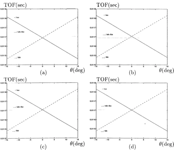
In the differentiation of target primitives which are introduced in the previous section, both TOF and amplitude characteristics must be used. In Figure 2.5 and 2.6, TOF characteristics for each primitive target are given over the range of —Oo < 0 < Oo where 0o is taken as 15". Note that the TOF characteristics of plane, corner, edge cind cylinder have the same form. Initially, to differentiate an acute corner from the rest of the tcirgets, these characteristics are used in Algorithm I which is introduced next. In the following, yUgorithm 1 is

based on TOF cornparisoji whereas Algorithms 2 and 3 are based on amplitude comparison of the return sigmils.

sec) TOF(sec)

Figure 2.5: The TOF characteristics of targets when the target is at r = 2 ni (a) plane (b) corner (c) edge with 6e = 90° (d) cylinder with ry. = 20 cm.

Algorithm 1: Acute Corner DifFereiitiation:

• if [iaaiO) - tabiO)] > kat aiid [hbiO) - tab{0)] > kt(Tt

then acute corner.

• if [tabiO) - taa{0)] > k at Or [tab{0) ~ tbb{0)] > hat then plane, corner, edge or cxjlinder.

where tab{0) denotes the TOF reading extracted at angle 0 from Aab(r,0,d, t) which is the signal transmitted by a and received by b.

TOF(sec) TOF(sec) -15 -10 -5 (a) (c) TOF(sec) -15 -10 -5 0 5 10 15 -15 -10 -5 0 5 10 15 0{deg) TOF(sec) (b) i>(deg) d(deg)

Figure 2.6: TOF characteristics of acute corner at r = 2 m with (a) Oc = 30“ (b) e, = 45“ (c) e, = 60“ (d) = 90“.

In this algorithm, at is the standard deviation of the TOF estimate which is in general nonlinearly related to the additive noise on the signal amplitude. This relationship is investigated in Appendix E. A multiple of at, ktat, is used to improve the robustness of the differentiation algorithiTi to noise.

The azimuth 0 and angle Oc of an acute corner can be estimated as:

0 -- sin ^ Or — sin“ ^ j r l - vL)(2,·^ + 2dr{rl + r-2J lyt 2 I (»'»2 ^aa

^ ^

where the geometry for Vaa and rtb are given in Appendix A. For ¿1 = 0“:

(2.5)

Cp{rabnb + íP - rl^ - r¡i,)

\J 4(?’a6 - nbY - (P (2.7)

To estimate range r for 6 ^ 0°, a, second-order polynomial must be solved:

o 9 cP

A:iP + 5a; + C = 0 where x = 2 r + — (2.8)

The coefficients of this polynomial are functions of Vaa, ri>b, rb,,. and d

given in Appendix C.

Note that when angle Oc is close to 90°, it is not possible to differentiate an acute corner by this algorithm. This algorithm can be used safely when 0c is in the range [0°,60°].

In the identification of the rest of the targets, amplitude charcicteristics given in Figure 2.7 must be used since their TOP charcicteristics have the same form. Amplitude characteristics of edges with various 0^ and cylinders with various 7'c are given in Appendix D. Based on the amplitude chciracteristics.

Algorithm 2 can be used to differentiate the phmar target from the rest of the target primitives.

Algorithm 2: Plane Differentiation:

• if [AaaiO) - AabiO)] > ^acta and [Ab6(f') - Ac,b{0)\ > kA(TA

then plane with

r = Ta + n

0 = sin_X f ^^6 '^ a

(2.9)

(2.10)

if [A.^l,(0) - AaJO)] > k^UA o r [Aa6(f') - A¡a(0)\ > kAUA then corner, edge or cxjlinder.

Here Aab{0), Aaa{0) and Abbi0) denote the maximum values of Aab{r, 0, d, t),

A„.a{r,0,d, t), Abb(r,0,d,t) at angle 0, whose functioned forms are provided in

Appendix A. The and r¡, are the perpendicular distances ol the respective transducers from the target whose geometry is also illustrated in Appendix A.

In this algorithm, different values for have been tested and the results are presented in Appendix B. Based on these results, it is appropriate to choose

kA = 1 .

In order to differentiate corner target primitive from edge and cylinder, amplitude measurements over the range —Oo < 0 < Oo must be taken. Since the maxima of Aaa{0)·, Aab{0)·, Ahh{0) are the same for a right-cUigle corner, this tyi^e of target can be differentiated from edge and cylinder by using Algorithm 3.

Algorithm 3: Corner Differentiation:

' if [max{Aaa(^)} - max{Afcfc(6<)} < cr^] and [max{Ab6(i^)} - rnax{/lafc(<?)} < œa]

then corner with

r — 0 = r2 _L r2 - ^ _{+ ^6 2} sm 2dr (2.11) (2.12)

else edge or cylinder.

In the above algorithm, max{Aaa.(^)} corresponds to the maximum ampli­ tude over the range —0o < 0 < 0o- With the given number of measurements, it is not possible to determine the orientation of the two planes forming the corner. Only the orientation of the line where the two planes intersect can be found with respect to the line-of-sight. To find the orientation of the planes, measurements which include reflections from the two constituent planes are necessary.

Referring to Figure 2.7, edge and cylinder targets can be distinguished over a small interval near 0 — 0°. At <? = 0°, ^„^(0) = Ao6(0) = /l6(,(0) for an edge but this equality is not true for a cylinder. Depending on the radius of the cylinder, it may be possible to differentiate edge and cylinder with this configuration of transducers. An edge is a target with zero radius of curvature. For the cylinder, the radius of curvature has two limits of interest. As —>■ 0 the characteristics of the cylinder approaches thcit of an edge. On the other hand as Tc —> oo, the characteristics is more similar to that of a plane. By assuming the target is a cylinder first cind estimating its I’cidius of curvature [28] it may be possible to distinguish these two targets for relatively large values

of Tc. For an edge, expressions for range r and azimuth 0 given in Equations

2 .ff and 2.12 are the same as in the case of a corner. In the case of cylinder,

in addition to range and azimuth, the radius of cylinder can also be estimated. These estimates are given by:

(2.13)

(2 .1 4 )

r ^ V ^ 2 e ^ s i i r ^ [ r l - r l ) + 2 r c i r a - n ■ 2^ ( n + T 2 ) 2 -- ( r l + r l ) 2 ( ^ r i, + V a — Amplitude Amplitude

Figure 2.7: Amplitude characteristics when the targets are cit r — 2 m(a) plane (b) corner (c) edge with 9e — 90° (d) cylinder with = 20 cm.

The ratio of transducer separation to operating range (i//?') is an important parameter in the differentiation of target primitives directly affecting how well these target primitives can be differentiated lyy their TOF and amplitude char­ acteristics. The further apart are the transducers, larger are the differentials in 'COF and amplitude as long as the sensitivity patterns of the targets overlap. T'his supports improved differentiation of the targets. In the limit as ^ 0 which corresponds to the case that either the transducers are too close together or the target is too far, the transducers behave as a single transducer and the differential signals are not reliable. This situation is equiv^alent to the case of trying to differentiate the targets using a single transd^rcer at a fixed location, which is not feasible. The effect of transducer separation d and range r on the maximum differentials is provided in Appendix A.

In this chapter, basic concepts of sonar sensing and target primitives used in this study are introduced. TOF and amplitude characteristics of each tar­ get tvpes are given and differentiation algorithms are developed. In the next chapter, these algorithms will be used by multiple decision-making sonars to identifv and locate an unknown target.

C hapter 3

LOGICAL SE N SIN G A N D

F E A T U R E F U S IO N OF

M U LTIPLE SE N SO R PA IR S

'riiis chcipter focuses on the development of a logical sensing module that |:)ro- duces evidential information from uncertain cind partial information obtained by multiple sonars at geographically different sensing sites. The Ibrniation of such evidential information is accomplished with the theory of belief functions. As a first attem pt, belief values are generated for each sensor pair cind assigned to tlie detected features: plane and corner. These features and their evidential metric obtained from multiple sonars are then fused using the Dempster-Shafer rule of combination. Acute corner is added as an additioiicil feature in the belief function approach and simulation results are presented.

3.1

L ogical Sensing

Belief function is a mapping from a class of sets to the interval [0,1] that assigns numerical degrees of support based on evidence [30]. This is a generalization of probabilistic approaches Tsirice one is allowed to model ignorance about a given situation. Unlike probability theory, a belief function brings a metric to the intuitive idea that a portion of one’s belief can be committed to a set but need not be also committed to its complement. In the target classification problem, ignorance corresponds to not having any information on the type of target that

the transducer pair is scanning.

To differentiate the target primitives, differences in the reflection charac­ teristics of these targets are exploited and formulated in terms of degrees of belief. This logical sensor model of sonar perception is novel in the sense that it models the uncertainties associated with the target type, its range and az­ imuth as detected by each sensor pair. The uncertainty in the measurements of each sonar pixir is represented by a belief function having target type or

ftaiure, and tcirget location r and 9 as focal elements with degrees of belief l)(.) associated with them:

BF = {feature, r, 9 ; b{ feature), b(r), b{9)} (3.1)

3.1.1

F eature Fusion from M u ltip le Sonars for P la n e-

C orner Id en tifica tio n

In this study, we first focus on differentiation of two of the target types intro­ duced, namely plane and corner. In section 3.1.3, the method will be extended to include the acute corner.

Logical sensing of target primitives is accomplished through a metric as degrees of belief assigned to plane and corner according to the amplitude and 'LOF characteristics of the received signals described in the previous chapter. 13a.sed on these characteristics, belief assignment to the feature focal element is nicide cxs follows

[AaaiO) - Aabi9)][M0) - ^akiO)] h

max[Aaa(i^) - Aah{9)] max[A66(i?) - (3.2) 6 (c) = /2 max

0

Aa|,i0)-Aaa{9)] + l·i[Aal,{O)-A^,b{O)]

Aab(0)-Aaa{O)] + h max[/lai,(0)-A6b(<?)] if h ^ 0 or ^ 0 J

if 7, = /3 = 0

where b{p) and 6(c) are beliefs assigned to plane and corner fecitures respectively

and Ii, I'z and /3 are the indicators of the conditions given below:

h =

/2 =

/3 =

1 if [Aaa{9) - Aai,(f')] > aiid [Abb{9) - Aab{9)] > kA(TA^,^

0 otherwise

1 if [Aab{9) - Aaa{0)\ > kAC^A

0 otherwise

1 if [Aab{9) - Abb{9)] > kA(TA

0 otherwise

(3.5)

Remaining belief is assigned to an unknown target, representing ignorcince, as:

b{u) = 1 - [b{p) + 6(c)] (3.7)

Decision of multiple sensor pciirs are fused with Dempster-Shafer rule of combination [30]. Consider belief functions obtained from two sonar pairs as independent sources of evidence (Table 3.1):

BFi = {/¿,6(/i)}·^^ = {2J,c ,u ;6 (p),6(c),6 (ri)l (3.8)

= {i'.nKi/i)}^! = { p ,c ,u ;6(p),6(c),6(u)} (3.9) Consensus is obtained ¿is the orthogonal sum:

B F - BFi © BF2 = {hk,b(Jik)}i=i = {p,c,u-,bc{p),bcic),bc(u)} (3.10)

which is both associative and commutative. The sequenticd co-rnbination of multiple bodies of evidence can be obtained for n sensor pairs as:

B F = {{{B F i © BF2) © B F s) ... © BFn)

Using the Dempster-Shafer rule of combination: ... . _ ZEh,=f,ng,Hfi)b{gj)

where J2J2hk=fingj=0 b(fi)b{gj) is a measure of conflict.

(3.11) (3.12) BFi BF2 plane blip) corner 6 1(c) unknown bi{u) plane b2{p) plane biip)b2{p) 0 bi{c)b2ip) plane bi{u)b2ip) corner 62(c) 0 bl{p)b2 ic) corner 6i(c)62(c) corner 6i(г¿)62(c) unknown b2(u) plane bi{p)b2{u) corner 6i(c)62(u) unknown 6i(li)62('u)

Table 3.1: Plane/corner differentiation by Dempster-Shafer rule of combina­ tion.

Referring to Table 3.1, intersection of events plane and unknown is plane, similarly intersection of events corner and unknown is corner. The intersection of plane and corner is an empty set.

The consensus belief function representing the feciture fusion is based on the fecitures of plane, corner and acute corner. The metrics of the fusion are:

bi{p)b2{p) + bi{p)b2{u) + bi{u)b2{p)

b{p) =

1 — conflict (3.13)

^ blic)b2ic) + bi{c)b2{u) + bi{u)b2{c)

1 — conflict

^ bi(u)b2iu)

b(u) = - — ^

1 - conflict (3.15)

In the above equations, the term “conflict” represents the disagreement in the consensus of two logical sensing units thus representing the degree of mismatch in the fusion of fecitures perceived at two different sensing sites. The metric evaluating conflict is expressed as:

conflict = 6i(p)6'2 (c) + bi{c)b2 {p) (3.16) Tlie beliefs are then rescaled after discounting this conflict and may be used in further data fusion processes.

3.1.2

Fusion o f R an ge and A z im u th E stim a te s

Assignment of belief to range and angle measurements is based on the simple observation that the closer the target is to the face of the transducer, the more accurate is the range reading, and the closer the target is to the line- of-sight of the transducer, the more accurate is the angle estimate. This is due to the physical i^roperties of sonar: signal amplitude decreases with r and with |t^|. At large ranges and larger angular deviations, sigiicil-to-noise ratio is smaller. Most accurate measurements are obtained along the line-of-sight (A = 0'^) and cit nearby ranges to the sensor pair. Therefore, belief assignments to range and azimuth estimates derived from the TOF measurements are made as follows [31]: ^ rnn.n' ^ b{r) = m

=

Note that, belief of r takes its maximum value of one when r = r„,,in its minimum value of zero when r = Vmax· Similarly, belief of 0 is one when

0 = 0" and zero when 0 =

±0o-Since each sensor pair takes measurements in own its sensor-centric coor­ dinate frame, the beliefs of range and azimuth information need to be first