An investigation of the leverage anomaly at Istanbul Securities Exchange

1 ,ν -'?· "ί' r‘" ■" ■ i ■’ i ^ t * i- ‘ '^ . % 7 .-i ··■ .■ ''!· ' , V ?»· '.' I " '*■· ·4». , ■'•r· . ' ■.. · , ^ Γ · .■. : » * Л ^ »■ r·· ' ^••: _ . · / / ¿ - ■' ' " ' ■ 5 Ä ) ( ^ - 5 ·

■ZS8

A3S

Ί9 Β 5

C ' /

AN INVESTIGATION OF THE LEVERAGE ANOMALY

AT ISTANBUL SECURITIES EXCHANGE

A THESIS

Submitted to the Faculty of Management

and the Graduate School of Business Administration

of Bilkent University

in Partial Fulfillment of the Requirements

For the Degree of

Master of Business Administration

By

i>0

CELAL AKKAYA ^

W6 *Sïùé.Ç ‘ / F ? Я S T v'V 4;· .'v' \) Л

I certify that I have read this thesis and in my opinion it is fiilly adequate, in scope and quality, as a thesis for the degree of the Master of Business Administration.

Assoc. Prof Kürşat Aydoğan

I certify that I have read this thesis and in my opinion it is fully adequate, in scope and quality, as a thesis for the degree of the Master of Business Administration.

I certify that I have read this thesis and in my opinion it is fully adequate, in scope and quality, as a thesis for the degree of the Master of Business Administration.

Assist. Prof Yüce

Approved for the Graduate School of Business Administration

A B S T R A C T

AN INVESTIGATION OF THE LEVERAGE ANOMALY AT ISTANBUL SECURITIES EXCHANGE

CELAL AKKAYA M.B.A. in Management

Supervisor: Assoc. Prof. K iirjat Aydogan December 1995, 55 pages

This study investigates the presence of ‘leverage effect’ at Istanbul Securities Exchange for the period January 1990 - December 1993.

Two leverage variables are used, the ratio of book equity to book assets, BE/A and the ratio of market equity to book assets, ME/A. We interpret BE/A as a measure of book leverage, while ME/A as a measure of market leverage.

In portfolio comparison methodology, each year, portfolios are formed according to the previous year’s ratio of book equity to book assets and ratio o f market equity to book assets and then the average monthly returns of the current year are compared. In addition, the cross-sectional regression approach of Fama-MacBeth (1973) is applied to determine which of the variables significantly explain the average return of stocks. The results show that a significant ‘leverage effect’ is not encountered at Istanbul Securities Exchange for the period of January 1990 - December 1993 in terms of book leverage and market leverage variables.

Ö Z E T

İSTANBUL MENKUL KIYMETLER BORSASINDA BİR ANOMALİ ARAŞTIRMASI

CELAL AKKAYA

Yüksek Lisans Tezi, İşletme Enstitüsü Tei Yöneticisi: Doç. Dr. K ürşat Aydoğan

Aralık 1995, 55 sayfa

Bu çalışma İstanbul Menkul Kıymetler Borsası’nda firma borçluluğu etkisi olup olmadığını Ocak 1990 - Aralık 1993 döneminde araştırmaktadır.

Borçluluk durumunun değişkenleri olarak, sermayenin kitap değerinin (book value) toplam aktiflere oranı, BE/A ve sermayenin pazar değerinin (market value) toplam aktiflere oranı, ME/A kullanılmıştır. BE/A kitap borçluluğu, ME/A pazar boçluluğu olarak tanımlanmıştır.

Portföy karşılaştırmalan ile yapılan analizde , her sene, hisse senetleri bir önceki senenin kitap borçluluk durumu ve pazar borçluluk durumu değerlerine göre sıralanarak portföyler oluşturulmuş ve portföylerin o seneki aylık getirileri karşılaştırılmıştır. Ayrıca, hangi değişkenlerin hisse senedi getirilerini istatiksel olarak açıkladığını bulabilmek için Fama-MacBeth(1973)’in kesit regresyonu metodu -kullanılmıştır. Ocak 1990 - Aralık 1993 döneminde, kitap ve pazar borçluluk durumu değişkenleriyle yapılan analizde, güçlü bir firma borçluluk etkisine rastlanmamıştır.

ACKNOWLEDGEMENTS

I wish to express my gratitude to Associate Professor Kür§at Aydogan for his supervision during the preparation of this thesis.

I also wish to express my thanks to my family for their invaluable supports all my life.

TABLE OF CONTENTS Abstract Özet Acknowledgements Table of Contents I. INTRODUCTION

II. THE PREVIOUS RESEARCH ON MARKET EFFICIENCY

III. DATA AND METHODOLOGY A. Data

B. Methodology

1. Calculation of ps

P age

2. Tests of Leverage Effect by Portfolio Comparison Approach 3. Tests of Leverage Effect By

Cross-sectional Regression Approach IV. FINDINGS

A. Summary Statistics About Data B. Results of t-tests Based on

Portfolio Comparison Approach C. Results of t- tests Based on

Cross-sectional Regression Approach V. CONCLUSIONS

VI. LIST OF REFERENCES Appendices I I iii iv 1 4 15 15 17 17 18 19 21 21 22 28 31 33 37 IV

I. INTRODUCTION

Capital markets serve to transfer funds between lenders (savers) and borrowers (producers) efficiently. A market is evaluated as allocationally efficient when prices are determined in a way that equates the marginal rates of return (adjusted for risk) for all producers and savers. But operational efficiency deals with the cost of transferring funds. In perfect capital markets, transaction costs are assumed to be zero. So, efficient capital markets imply operational efficiency as well as asset prices that are allocationally efficient. According to market efficiency hypothesis, security prices reflect all relevant information in an efficient market.

Several research have been conducted on market efficiency tests. The 1970 review by Fama divides work on market efficiency into three categories;

(1) weak form tests (How well do past returns predict future returns?)

(2) semi-strong form tests (How quickly do security prices reflect public information announcements?)

(3) strong-form tests (Do any investors have private information that is not fully reflected in market prices?) [Fama 1991]

But the first category now covers the more general area of tests for return predictability. It also includes the work on forecasting returns with variables like dividend yield and interest rates. However, an asset pricing model and capital market efficiency are joint and inseparable hypothesis. If capital markets are inefficient, then the assumptions of the asset pricing model are invalid and a different model is required. If the asset pricing model is inappropriate, even though capital markets are efficient, then the asset pricing model is the wrong tool to use in order to test for efficiency. So tests are only conducted on the reflection of information in the context of equilibrium pricing model. In addition, the discussion of predictability also considers the cross-sectional predictability of returns, that is, tests of asset pricing models and the anomalies (like the size effect) discovered in the tests.

One of the asset pricing models is the model of Sharpe(1964), Lintner(1965) and Black(1972). The SLB model gave a summary measure of risk, market (3 interpreted as market sensitivity. It suggested that (1) expected returns are a positive linear function of market beta (the covariance of a security's return with the return on the market portfolio divided by the variance of the market return) and (2) (3 is the only measure of risk needed to explain the cross-section of expected returns.

The empirical attacks on the SLB began in the late 1970’s with studies that identify variables that contradict the model's prediction that market ps suffice to describe the cross-section of expected returns. In an efficient market, if SLB is correct, we do not expect an anomaly to explain the variation in cross-sectional returns.

Size effect, dividends/price (D/P) ratio effect, leverage effect, book/market value (B/M) effect and eamings/price (E/P) ratio effect are identified and determined as the different types of anomalies in the cross-section of regression of expected returns. Leverage effect refers to average returns of stocks with high leverage are substantially higher than that of the stocks with low leverage.

At Istanbul Securities Exchange, some studies has been conducted about the presence of weak and semi-strong form efficiency. Civelekoölu(1993) used the cross-sectional predictability of returns with an asset pricing model and the anomalies for the first time. He has found that there exists a weak "E/P effect" in the years 1991 and 1992. However, a significant "Size effect" is not encountered at ISE as opposed to the case in developed capital markets.

In this study, the aim is to jointly test the market efficiency with an asset pricing model by investigating the presence of a leverage anomaly at ISE for the period January 1990 - December 1993 by using two variables, book leverage and market leverage.

The arrangement of this thesis is in the following manner. In Section 2, the empirical studies on anomalies and a rewiew of literature about market efficiency is presented. In section 3, the data and methodology used in this study are explained. In section 4, leverage effect is tested by portfolio comparison approach and by cross-sectional regression approach. The findings are also discussed for market leverage and book leverage. In Section 5 the findings are presented with a summary of the model and the results.

II. THE PREVIOUS RESEARCH ON MARKET EFFICIENCY

The purpose of capital markets is to transfer funds between lenders (savers) and borrowers (producers) efficiently. In a somewhat limited sense, efficient capital markets imply operational efficiency as well as asset prices that are allocationally efficient. Asset prices are correct signals in the sense that they fully and instantaneously reflect all available relevant information and are useful for directing the flow of funds from savers to investment projects that yield the highest return (even though the return may reflect monopolistic practices in product markets). Capital markets are operationally efficient if intermediaries, who provide the service of channeling funds from savers to investors, do so at the minimum cost that provides them a fair return for their services.

Fama(l970,1976) has done a great deal to operationalize the notion of capital market efficiency. He defines three types of efficiency, each of which is based on a different notion of exactly what type of information is understood to be relevant in the phrase "all prices fully reflect all relevant information."

l.W eak Form Efficiency; No investor can earn excess returns consistently by developing trading rules based on historical price or return information. In other words, the information in past prices or returns is not useful or relevant in achieving excess returns. In a weakly efficient

market, present prices reflect all information contained in the record of past prices, that is, investors cannot consistently earn abnormal returns by observing the past prices.

2. Semi-strong Form Efficiency; No investor can earn excess returns consistently from trading rules based on any publicly available information. Examples of publicly available information are annual reports of companies, investment advisory data such as "Heard on the Street" in the Wall Street Journal, or ticker tape information. In a semistrongly efficient market, prices reflect all available information, that is, security prices adjust rapidly and correctly to the announcement of all available information.

3. Strong Form Efficiency; No investor can earn excess return consistently using any information, whether publicly available or not. In a strongly efficient market, present prices reflect all information, both privately held and insider information together with publicly available information.

Early research on weak-form efficiency only concerns with the forecast power of past returns. But this category now covers the more general area of tests for return predictability, which also includes the work on forecasting returns with variables like dividend yields and interest rates. Since market efficiency and equilibrium pricing issues are inseperable, the discussion of predictability also considers the cross-sectional predictability of returns, that is.

tests of asset pricing models and the anomalies (like the size effect, the leverage effect) discovered in the tests.

According to the CAPM, the only relevant parameter necessary to evaluate the expected return for every security is its systematic risk. Therefore if the CAPM is true and if markets are efficient, the expected return of every asset should fall exactly on the security market line. Any deviation from the expected return is interpreted as an abnormal return, and can be taken as evidence of market inefficiency if the CAPM is correct. However, CAPM and capital market efficiency are joint and inseperable hypotheses. If capital markets are inefficient, then the assumptions of the CAPM are invalid and a different model is required. And if the CAPM is inappropriate, even though capital markets are efficient, then the CAPM is the wrong tool to use in order to test for efficiency.

The joint hypothesis problem is more serious obstacle to inferences about market efficiency as it’s mentioned in the CAPM model. But market efficiency per se is not testable. It must be tested jointly with a model of equilibrium, an asset pricing model. According to the 1970 review [Fama(1970)], what can be only tested is whether information is properly reflected in prices in the context of an asset pricing model. As a result, if an anomalous evidence is found on the behavior of security returns, it is ambiguous that market is inefficient or the model of equilibrium, the asset pricing model is bad. [Fama( 1991)]

The asset pricing model of Sharp (1964), Lintner (1965) and Black (1972) has long shaped the way academics and practioners think about average returns and risk. The central prediction of the model is that the market portfolio of invested wealth is mean-variance efficient in the sense of Markowitz (1959). The efficiency of the market portfolio implies that (a) expected returns on securities are a positive linear function of their market P (the slope in the regression of a security's return on the market's return) and (b) market Ps suffice to describe the cross-section of expected returns.

Black , Jensen and Scholes (1972) and Fama and French (1973) find that, as predicted by the SLB model, there is a positive simple relation between average stock returns and P during the pre-1969 period. But Reinganum (1981) and Lakonishok and Shapiro (1986) and Fama and French (1992) find that the relation between P and average return disappears during the more recent 1963-1990 period, even when P is used alone to explain average returns. Fama and French (1992) show that the simple relation between P and average return is also weak in the 50 year 1941-1990 period. Tests do not support the most basic prediction of the

SLB model, that average stock returns are positively related to market Ps.

There are other empirical contradictions of the SLB model . The most prominent is the size effect of Banz (1981). He finds that market equity, ME (a stock's price times shares outstanding), adds to the explanation of the cross-section of average returns provided

by market (3s. Average returns on small (low ME) stocks are too high given their (3 estimates, and average returns on large stocks are too low.

Statman (1980) and Rosenberg, Reid, and Lanstein (1985) find that average returns on U.S stocks are positively related to the ratio of a firm's book value of common equity ,BE, to its market value, ME. Chan, Hamao, and Lakonishok (1991) find that book to market equity, BE/ME, also has a strong role in explaning the cross-section of average returns on Japanese stocks. Chan, Hamao and Lakonishok (1991) and Fama (1991) find that BE/ME has strong explanatory power; controlling for (3, higher BE/ME are associated with higher expected returns.

Basu (1983) shows that eamings-price ratios (E/P) help explain the cross-section of average returns on U.S stocks in tests that also include size and market p. Ball (1978) argues that E/P is a catch-all proxy for unnamed factors in expected returns; E/P is likely to be higher (prices are lower relative to earnings) for stocks with higher risks and expected returns, whatever the unnamed sources of risk.

Fama and French (1988) use D/P to forecast returns on the value-weighted and equally weighted portfolios of NYSE stocks from 1 month to 5 years. They find that D/P explains small fractions of monthly and quarterly return variances. However, fractions of variance explained grow with the return horizon and are around 25% for 2 to 4 year returns.

DeBondt and Thaler (1985-1987) find that the NYSE stocks identified as the most extreme losers over a 3- to 5- year period tend to have strong returns relative to the market during the following years. On the contrary, the stocks that are extreme winners tend to have weak returns relative to the market in subsequent years.

Zarowin (1989) finds no evidence for the DeBondt- Thaler hypothesis that the winner- loser results are because of overreaction to extreme changes in earnings. He argues that the winner-loser effect is related to the size effect of Banz (1981).

Another contradiction of the SLB model is the positive relation between leverage and average return documented by Bhandari (1988). It is plausible that leverage is associated with risk and expected return, but in the SLB model, leverage risk should be captured by market P . Bhandari finds, however, that leverage helps explain the cross-section of average stock returns in tests that include size(ME) as well as p. Firm's debt equity ratio (DER) is used as the natural proxy for the risk of common equity of a firm. An increase in the DER 6f a firm increases the

risk of its common equity. Though it does not follow that, cross-sectionally, the common equity of a higher DER firm always has higher risk since the firm-level may vary, DER is expected to be positively correlated to the risk of common equity across firms. Thus, DER is used as a proxy for the risk of common equity when an adequate measure of risk is not known or cannot be calculated from available information. In conjunction with the estimation errors in P, use of a proxy for the market portfolio, and possible changes in P over time suggests that P alone may

not be as good a proxy for true P during test period. For example, to the extent that the firm P is relatively stable, a higher DER during the test period relative to that during the P calculation period will indicate a higher-than-estimated common equity p during the test period in addition to (P; an estimate of P, is used to control for P, based on a market proxy and calculated from a period termed the P calculation period, which does not overlap with the corresponding test period). Also, usually the data requirements are such that the P calculation period for a firm excludes the period surrounding the time it drops out of the data set. Then the combination of low return on the market proxy and low "residual" return for a firm is more likely to be excluded from P calculation since such a combination is more likely to cause that firm to go bankrupt and drop out. This sample selection bias will bias P downward in all practical cases. Since the probability of bankruptcy increases as DER increases, a higher DER may indicate more downward bias in P .

Bhandari (1988) concluded,that the expected common stock returns are positively related to the ratio of debt (non-common equity liabilities) to equity, controlling for the P and firm size and including as well as excluding January, though the relation is much larger in January. This relationship is not sensitive to variations in the market proxy, estimation technique, etc.

B ook value o f total assets - B o o k value o f com m on equity

DER=-Market value of common equity

Fama and French (1992) find that unlike the simple relation between P and average return, the univariate relations between average return and size , leverage, E/P, and BE/ME are strong. Their bottom line results are; (a) P does not seem to help explain the cross-section of average stock returns , and (b) the combination of size and book to market equity seems to absorb the roles of leverage and E/P in average stock returns, at least during 1963-1990 sample period. They used two variables as a measure of leverage effect in the Fama-MacBeth regressions. The ratio of book assets to market equity , A/ME, and the ratio of book assets to book equity, A/BE. A/ME and A/BE are interpreted as a measure of market leverage and book leverage. The average slopes for the two leverage variables are opposite in sign but close in absolute value. So the difference between market and book leverage that helps explain average returns. But the difference between market and book leverage is book-to-market equity, In(BE/ME)=In ( A/ME) - In (A/BE). A high book-to-market ratio says that a firm's market leverage is high relative to its book leverage; the firm has a large amount of market imposed leverage because the market judges that its prospects are poor and discounts its stock price relative to book value. So, tests suggest that the relative-distress effect, captured by BE/ME, can also be interpreted as an involuntary leverage effect, which is captured by the difference between A/ME and A/BE.

Some empirical tests are also achieved to investigate the market efficiency at Istanbul Securities Exchange (ISE). On these studies, market is generally found as inefficient in terms of weak-form efficiency and strong-form efficiency.

Başçı (1989) carried out a study on distributional and time series behavior of common stock returns at ISE for the period 1986-1988. He finds that published past price information cannot be used to obtain better forecasts of future prices. This observation is parallel with the random walk behavior, that is the weak form efficiency. However, the test of variance-time function indicate significant long term dependence for most stocks which is against the weak form efficiency hypothesis.

Alparslan (1989) carried out a study by applying weak-form efficiency tests at ISE. He used statistical tests of independence (autocorrelation and run tests) and tests of trading rules (filter rules) in these tests. Runs and autocorrelation tests could not reject the weak-form efficiency. However, the results of the filter tests show that for some stocks the market could have been beaten by an investor. Alparslan concluded that the market is inefficient in the weak

sense.

Ünal (1992) uses daily adjusted closing prices of twenty major stocks for the period 1986-1991. The tests are carried out on independence , randomness and distribution of daily

prices. He also tests whether some mechanical trading rules consistently and significantly profitable over a buy-and-hold policy by trade rules tests. All his results are against weak-form efficiency at ISE.

Çadırcı (1990) carried out a study as an empirical test on semi-strong form efficiency. Market adjustment to the release of stock dividend / rights offering information for the stocks listed at ISE first market for the period 1986-1989 is investigated. The results of her study demonstrates that the adjustment process is slow and, positive cumulative abnormal returns are observed after the event date. So, she rejects the market efficiency in semi-strong form efficiency at ISE.

Civelekoğlu (1993) carried out a study by jointly testing the market efficiency with an asset pricing model by investigating the presence of a size efifect and E/P effect anomalies at ISE for the period January 1990 - December 1992. The results reveal that there exists a weak "E / P effect" in the years 1991 and 1992. However, a significant "size effect" is not encountered at ISE as opposed to the case in developed capital markets.

Kurdoğlu (1994) investigated the performance of portfolios consructed by single index model with historical (least squares regression) ^s and estimated future Ps by Vasieck’s Bayesian Estimation Technique. The Ps of the stocks were very volatile. Even if previous studies have

shown that Vasieck’s adjusted P outperforms the historical one, in this study, this could’nt be shown for ISE.

Timur (1993) found that the information reflected in the past prices of the . monetary variables have significant effects on the ISE composite index.

Many of the front line empirical anomalies in finance (like the size effect) come out of tests directed at asset pricing models. Given the joint hypothesis problem, one can't tell whether such anomalies result from misspecified asset pricing models or market inefficiency. This ambiguity is sufficient justification to review tests of asset pricing models.

The aim of this study is to jointly test the market efficiency with an asset pricing model by investigating the presence of a leverage effect anomaly at ISE for the period January 1990 - December 1993.

I1I.DATA AND METHODOLOGY

A. Data

The data used in this study includes the monthly returns of the stocks listed at the Istanbul Securities Exchange ( ISE ) and the leverage figures over the period January 1988 to December 1993. The stocks that satisfy the following condition are considered in the study. The condition is to have 36 consecutive monthly returns starting 24 months before and ending 12 months after the beginning of the year T (T= 1990.. 1993). Financial firms are excluded because the high leverage that is normal for these firms probably does not have the same meaning as for

nonfmancial firms, where high leverage more likely indicates distress.

Adjusted monthly closing price figures , book value of total assets and book value of common equity values as of the last trading day of year T, are obtained by using data from the monthly bulletins of ISE and balance sheets that are publicly available at SPK. The above mentioned figures are used in the calculation of monthly returns and leverage ratios of the stocks.

For monthly "risk-free rate", monthly returns of the treasury bills with three months of maturity are used. This data is taken from the monthly bulletins of Central Bank of Turkey.

The firms that satisfy the condition at ISE are taken into consideration. For the tests in 1990, total number of stocks traded during the year is 114, 37 of them satisfy the condition. For the year 1991, 45 stocks out of 142, for the year 1992, 62 out of 152 satisfy the condition. In

1993, 85 stocks have 36 consecutive monthly returns. (Appendix 1 through 4)

Book leverage of a stock for the year T is computed as the ratio of book equity to total assets as of the last trading day of the year T-1. Market leverage of a stock for each month of the year T is also computed as the ratio of market equity to total assets. Market equity figures for each month of year T are obtained in the following way. For each month of test year T, total number of shares outstanding in year T-1 are multiplied with the closing price of the stock in the previous month. Total number of shares outstanding are also calculated by dividing paid-in- capital figures in year T-1 by 1000 that is taken as a nominal value of one stock.

B.Methodology

1. Calculation of Ps:

For the calculation of P coefficients for individual stocks, 24 months of data prior to year T are used to estimate the market model regression.

Rj f R f t= “ jt+ Pjt (Rm t ■ R f t)+ t t = T-24,... ,T-1 (1)

where

Rj t i return on stock j in month t

Rm t : return on equally weighted market portfolio in month t

R f t 5 return on risk free asset in month t measured as monthly return of quarterly treasury bills.

Pjt : stock j's relative risk for year T (estimated OLS slope)

« jt : differentials or abnormal return for stock)

t : month t of year T (T=1988..1992)

2. Tests of Leverage Effect by

Portfolio Comparison Approach:

The methodology of this section is based on the studies of Basu(1983) and Reinganum (1981). The leverage ratios are calculated for each year T ( T=1990.. 1993) with the figures of year T-1. Then the stocks are sorted in ascending order. According to its leverage ratio, each stock is assigned one of three portfolios. For example; portfolio PI contains highly risky stocks with the lowest leverage ratios (since as (equity/total assets) ratio decreases, (debt/total assets) ratio increases for the same stock), whereas P3 contains the stocks with highest leverage ratios.

The above portfolio formation procedure is repeated each year from 1990 to 1993. So the portfolio composition changes each year. The reason beyond why we form three portfolios is to make meaningful statistical inferences from these data. Tests are applied between the low leveraged portfolio (LLP) and the high leveraged portfolio (HLP) by discarding the middle leveraged portfolio (MLP).

With this data, the null hypothesis that whether there exists a difference in average returns and mean |3s between high and low leverage portfolios is tested with a t-test at the 0.05 significance level. In addition, whether the abnormal returns of the portfolios formed are different

than zero or not is also tested with a t-test. Abnormal return can be defined as the difference between average monthly return of a portfolio formed based on book leverage or market leverage and average monthly return of the equally weighted market portfolio.

2. Tests of Leverage Effect by Cross-sectional Regression Approach:

The. methodology of this section is based on the cross-sectional regression approach of Fama and MacBeth (1973). The following linear relationship is the assumption;

E(Ri)= XQ+ xiPi+ x2LRi where

E(Rj) = expected return on stock i

XQ = expected return on zero-beta portfolio

XI = expected market risk premium

*2 = constant as a measure of contribution leverage ratio to the expected return of stock i.

LR[ = natural logarithm of market leverage ratio of stock i

Pi = stock i's relative risk (estimated OLS slope)

The parameters in the linear equation will be estimated by using that past data. Fama (1976) used a constrained optimization procedure to generate minimum variance portfolios with mean returns. The cross-sectional regression will be performed on the defined linear relation on a period by period basis.

Each month the cross-section of returns on stocks are regressed on the stock P and leverage ratio. P and leverage ratio are the hypothesized factors to explain the expected returns. At the beginning of each year T (T= 1990 ... 1993), the hypothesized factors P and leverage ratios are updated. As in the previous test,P is the slope of the regression line of the most recent 24 months time series monthly return data of each stock in the monthly return data of equally weighted market portfolio. Leverage ratio is also calculated from the figures as it’s mentioned in the portfolio comparison approach.

The time series mean of the monthly regression slopes between Jan. 1990 and Dec. 1993 provides standard Fama-MacBeth tests of which explanatory variables, P and/or leverage ratio have nonzero expected premiums over the test period. So, null hypothesis that mean of time series regression coefficient (x) is

zero tested for P and leverage ratios for each Xj, i=l,2.

IV.FINDINGS

A. Summary Statistics About Data

Not all stocks traded at ISE are used in tests. As described before, for a stock to be taken in the sample, it should have 36 consecutive monthly returns starting 24 months before and ending 12 months after the beginning of year T (T=1990, 1991, 1992, 1993). Number of securities that satisfy condition is 37 for the year 1990. This number is 45, 62 and 85 for the years 1991,1992 and 1993 respectively.

For each stock in the sample, descriptive statistics about their monthly returns are given in Appendix 1, 2, 3, 4. They consist of average, minimum, maximum, standard deviation and median of the monthly returns for each stock.

The regression results for each test year T to determine the market risk of each security are presented in Appendix 7, 8, 9, 10. 24 monthly returns of stocks before the year are used as the data in the calculations. The monthly closing prices are adjusted for any stock-split, rights offering and dividend payments, p and a coefficients, F values and their t-statistics are presented in the above mentioned appendices.

All the t-ratios for P are found to be significant. However, t-ratios for a coefficients are found to be insignificant. Calculated F-values are greater than the critical F values.

So the regression is considered as significant. Finally, t-statistics for a means that the stocks are neither underpriced nor overpriced.

B. Results of t-tests Based on Portfolio Comparison Approach

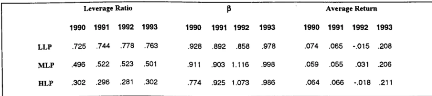
In each test year T (T= 1990 .. .1993), 3 portfolios (HLP, MLP, LLP) are formed based on book and market leverage ratio of stocks as described in the methodology section. Summary statistics about those portfolios are summarized in Table 1. They include the average book equities, market equities, total assets, leverage ratios with the average 3 coefficients and the monthly returns for the year T.

Years 1990 1991 1992 1993

No.of Stocks Included In The Portfolios 12

15

21

28

As it can be seen in the above summary table, the minimum number of stocks in the portfolios is 12 in 1990 and the maximum number of stocks is 28 in 1993.

TABLE 1. SUMMARY STATISTICS

SORTED ON BOOK LEVERAGE

LLP MLP HLP

Leverage Ratio Average Return 1990 1991 1992 1993 1990 1991 1992 1993 1990 1991 1992 1993

.725 .744 .778 .763 .928 .892 .858 .978 .074 .065 -.015 .208

.496 .522 .523 .501 .911 .903 1.116 .998 .059 .055 .031 .206

.302 .296 .281 .302 .774 .925 1.073 .986 .064 .066 -.018 .211

SORTED ON MARKET LEVERAGE

Leverage Ratio Average Return 1990 1991 1992 1993 1990 1991 1992 1993 1990 1991 1992 1993 LLP .931 1.001 1.089 3.246 .904 .924 1.066 .964 .025 .274 .101 .112

MLP .341 .320 .402 .943 .872 .951 .946 .905 .606 .515 -.052 .184

HLP .150 .135 .132 .283 .995 .942 .881 .826 .048 .006 -.050 .169

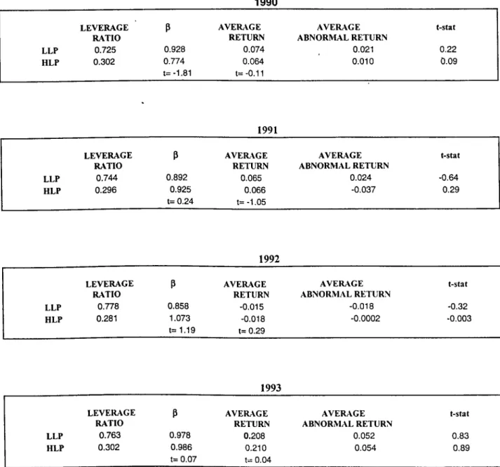
t-statistics indicating whether the mean returns of the portfolios are equal or not and t-statistics showing whether the abnormal returns of the portfolios (average monthly portfolio return minus average return on equally weighted market portfolio) are different from zero or not are presented in Table 2 and Table 3.

According to the results, t-statistics suggest that there is no “Book Leverage Effect” and “Market Leverage Effect” for the stocks traded at ISE, that is the stocks with high leverage do not outperform the stocks with low leverage.

In terms of book leverage, in 1990, low leveraged firms earned average monthly return of 7.4% while the average monthly return of high leveraged firm 6.4% as opposed to the expectations. But in 1991 and 1993, high leveraged firm returns were slightly above the ones of the low leveraged firm. In 1992, they were slightly below; -1.81% versus -1.53%.

With market leverage figures, in 1990 and 1993, high leveraged firm returns were considerably above the returns of the low leveraged firms. But even in these years’ tests, leverage effect is not encountered.

TABLE 2. LOW AND HIGH LEVERAGE PORTFOLIOS

SORTED ON BOOK LEVERAGE

1990 LEVERAG E R A T IO P AVERAGE RETURN AVERAG E A B N O R M A L RETURN t- s ta t LLP 0.725 0.928 0.074 0.021 0.22 HLP 0.302 0.774 t=-1.81 0.064 t= -0.11 0.010 0.09 1991

LEVERAG E P AVERAGE AVERAGE t- s ta t

R A T IO RETURN A B N O R M A L RETURN

LLP 0.744 0.892 0.065 0.024 -0.64

HLP 0.296 0.925 0.066 -0.037 0.29

t= 0.24 t=-1 .0 5

1992

LEVERAG E P AVERAGE AVERAG E t- s ta t

R A T IO RETURN A B N O R M A L RETURN LLP 0.778 0.858 -0.015 -0.018 -0.32 HLP 0.281 1.073 -0.018 -0.0002 -0.003 t= 1 .1 9 t= 0.29 1993 LEVERAG E R ATIO P AVER.VGE RETURN AVERAGE A B N O R M A L RETURN t-s ta t LL P 0.763 0.978 0.208 0.052 0.83 HLP 0.302 0.986 t= 0.07 0.210 t:= 0.04 0.054 0.89 Note:

1) t- statistics for P and average return of portfolios are for the null hypothesis that meanP and return ofhigh and low leverage portfolios are equal

2) t-statistics for average excess return of portfolios are for the null hypothesis the mean excess return of the portfolios are zero.

TABLE 3. LOW AND HIGH LEVERAGE PORTFOLIOS

SORTED ON MARKET LEVERAGE

1990 LEVERAG E R ATIO P AVERAGE RETURN AVERAGE A B N O R M A L RETURN t-s ta t LLP 0.931 0.904 0.025 -0.02 9 -0 .0 3 3 HLP 0.150 0.995 t= 6.13 0.048 t= 0.66 0.0 42 0.3 7 1991 LEVERAG E R A T IO P AVERrVGE RETURN AVERAGE ABN O R M AL RETURN t- s ta t LLP 1.001 0.924 -0.009 -0.051 -0.65 HLP 0.135 0.944 t=1.41 0.006 t= 0.18 -0.03 6 -0.3 9 1992 L E V E R A G E R A T IO P A V E R A G E RETU R N A V E R A G E A B N O R M A L R E T U R N t-stat LLP 1.089 1.066 -0.053 -0.05 6 -0.9 3 HLP 0.132 0. 881 t=-7.93 -0.050 t= 0.05 -0.05 2 -0.85 1993 LEVERAG E R A T IO P AVERAGE RETURN AVERAGE A B N O R M A L RETURN t-sta t LLP 3.246 0.964 0.112 -0.04 4 -0.7 5 HLP 0.283 0.826 t= -5 .4 4 0.169 t= 0.95 0.0 13 0.21 Note:

1) t-statistics for P and average return of portfolios are for the null hypothesis that mean P and return of high and low leverage portfolios are equal.

2) t-statistics for average excess return of portfolios are for the null hypothesis thatmean excess return of the portfolios are zero.

For the mean Ps of high and low book leverage portfolios, tests in 1990, 1991, 1992, 1993 indicated that they are not different from each other. But it is interesting that mean P of the low leveraged firms is smaller than the one of high leveraged firms except 1990.

In the tests of the mean ps of high and low market leveraged portfolios, it can be concluded that they are different from each other in 1990 and 1992. In 1990 and 1991, the mean ps conform with the expectations that high leveraged firms has higher risk level and accordingly higher ps than ps of low leveraged firms. But in years 1992 and 1993, the figures is opposed to the expectations.

Average abnormal return data shows that in 1990, high book leveraged stocks earned average monthly abnormal return 1% while this number is only 2.1% for low book leveraged stocks, t-statistics testing the null hypothesis that abnormal returns for low and high market leveraged portfolios in 1990 are -0.3250 and 0.3682 respectively. For the period between January 1990-December 1993 , we can not conclude that high leveraged firms outperform above the equally weighted market portfolio.

Book leverage figures are minimum 0.2814 in 1992, and maximum 0.7782 in the same year and portfolio average does not change slightly over the years. But in the analysis with market leverage, low leveraged portfolio changes from 0.9305 in 1990 to 3.2458 in 1993. So the use of market leverage increases the sensitivity of the analysis.

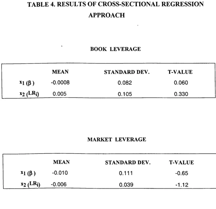
C. Results of t-tests Based on Cross-sectional Regression Approach

For each month of test year T (T= 1990... 1993), cross-section of monthly stock returns are regressed on P and leverage ratio as described in the methodology section. P and leverage ratio data for each stock are updated every year.

Average slopes of each monthly cross-sectional regressions with value of the regressions are presented in Appendix 5 and Appendix 6. Mean of each monthly Fama-MacBeth coefficients together with their t-statistics testing whether they are equal to zero or not are presented in Table 3. The results reveal that all of the variables, P or leverage ratio are found to be insignificant.

A major shortcoming of using Fama-MacBeth approach is that the approach assumes that the coefficients estimated every period are drawn from a stationary distribution. Changes over time in the levels of the explanatory variables will invalidate this assumption. The use of estimated Ps rather than true Ps are another drawback in the cross-sectional regressions.

In addition to above mentioned shortcomings, due to small number of stocks in the sample, individual stocks are used in this test rather than portfolios which, in fact, give better results. (Fama and French (1992)). Therefore, values are quite low in each monthly cross-sectional regression.

APPROACH

TABLE 4. RESULTS OF CROSS-SECTIONAL REGRESSION

BOOK LEVERAGE

MEAN STANDARD DEV. T-VALUE

^i(P)

-0.0008 0.082 0.060

%2 (LRi) 0.005 0.105 0.330

MARKET LEVERAGE

MEAN STANDARD DEV. T-VALUE

*1 (P) -0.010 0.111 -0.65

12 (LRi) -0.006 0.039 -1.12

In the analysis, P is also found to be insignificant. So the results of this approach are not consistent with the findings of Fama and MacBeth (1973) and Black, Jensen and Scholes (1972). However, our findings on the relationship between P and average return are similar to the more recent work by Fama and French (1992), and Lakonishok and Shapiro.

The existence of leverage effect is investigated for common stocks traded in Istanbul Stock Exchange for the period January 1990 - December 1993. Two different methods are implemented for this purpose.

First method makes use of a comparison of the average return and other characteristics of portfolios of common stocks based on leverage ratios. Due to insufficient number of stocks that meet the criteria to be included in the test sample in each year, HLP and LLP are formed each year where HLP consist of high leveraged stocks (with low leverage ratio) and LLP consist of low leveraged stocks (with high leverage ratio). This procedure is repeated for both market leverage and book leverage. The average returns of these portfolios are compared in each year from 1990 to 1993 and the null hypothesis of the mean difference in returns is zero is tested.

The findings of the comparison of portfolios with different leverage ratio and the market value shows no evidence for the presence of a leverage effect at ISE. However with market leverage figures, in 1990 and 1993,high leveraged firm returns were considerably above the returns of the low leveraged firms.But even in these year’s tests, leverage effect is not encountered in tests.

V. CONCLUSIONS

The second method implemented is the procedure of Fama-MacBeth (1973) applied to the stocks for the same period. Each month from January 1990 to December 1993, monthly stock returns are regressed on the hypothesized variables of estimated (3s and leverage ratio of the common stocks. Then, the average of the slopes of these regressions form a time series data that indicates which variables are significant in explaining the average monthly returns of the common stocks.

The results of Fama-MacBeth procedure shows that (3 and leverage ratio are insignificant in explaining the average monthly returns of the common stocks as it is consistent with the results of the first method.

With the results of two approaches, it can be concluded that there is no leverage effect at ISE for the period January 1990 - December 1993. Even the use of updated (3s and market leverage figures has not improved the results in such a way that to conform with the studies of Bhandari (1988) and Fama and French (1992).

Alparslan, S.M. (1989) “ Tests of weak form efficiency in Istanbul Stock Exchange”, Thesis submitted to the Department of Management and the Graduate School of Business Administration of Bilkent University.

Ball, Ray. (1978) “ Anomalies in relationships between securities’ yields and yield surrogates”. Journal of Financial Economics 6,159-178.

Banz, Rolf W. (1981) “The relationhip between return and market value of common stocks”. Journal of Financial Economics 9, 3-18.

Basel E. (1989) “The behavior of stock returns in Turkey: 1986-1988”, Thesis submitted to the Department of Management and the Graduate School of Business Administration of Bilkent University.

Basu, Sanjoy. (1983) “ The relationship between earnings yield, market value, and return for NYSE common stocks:Further evidence”. Journal of Financial Economics 12,

129-156.

Bhandari, Laxmi Chand. (1988) “Debt/Equity ratio and expected common stock retums:Empirical Evidence”, Journal of Finance 43, 507-528.

Black, Fischer. (1972) “Capital market equilibrium with restricted borrowing”. Journal of Business 45,444-455.

Black, Fischer, Michael C. Jensen, and Myron Scholes. (1972) “The capital asset pricing model: Some empirical tests, in M. Jense, ed.” Studies in the Theory of Capital Markets (Praeger, New York, NY)

VI. LIST OF REFERENCES

Campbell, John Y., and Robert Schiller.(1988) ” Stock prices, earnings and expected dividends”. Journal of Finance 43,661-676.

Cadirci, Begum. (1990) “The adjustment of security prices to the release of stock dividend/ rights offering information”. Thesis submitted to the Department of Management and the Graduate School of Businesss Administration of Bilkent University.

Chan, Louis K., Yasushi Hamao and Josef Lakonishok, (1991) “Fundamentals and stock returns in Japan”, Journal of Finance 46, 1739-1789.

Christie, Andrew A. and Michael Hertzel, ( 1981 ) “ Capital asset pricing anomalies: Size and other correlations “ , Manuscript ( University of Rochester, Rochester, NY)

Civelekoglu, Hakan. (1993) ” An investigation of anomalies at ISE: Size and E/P effects”. Thesis submitted to the Department of Management and the Graduate School of Businesss Administration of Bilkent University.

DeBondt, Werner F.M., and Thaler, Richard H. (1987), “Further evidence on investor overreaction and stock market seasonality”. Journal of Finance, 42, 557-581.

Fama, Eugene F. (1970) “ Efficient capital markets:A review of theory and empirical work”. Journal of Finance 25, 383-417.

Fama, Eugene F. (1991) “ Efficient capital markets: II ”, Journal of Finance 46, 1575-1617.

Fama, Eugene F., and MacBeth James D. (1973) “Risk, Return and Equilibrium: Empirical Tests”, Journal of Political Economy 31; 607-36

Fama, Eugene F., and Kenneth R. French. (1988) “ Dividend yields and expected stock returns”, Journal of Financial Economics 25,23-49.

Fama, Eugene F., and Kenneth R. French. (1992) ’’The cross-section of expected stock returns”. Journal of Finance 47,427-465.

Jensen, Michael C. (1978) “ Some anomalous evidence regarding market efficiency “, Journal of Financial Economics 6, 96-101.

Jobson J.D. and Korkie B. (1982) “Potential Performance and Tests of Portfolio Efficiency”, Journal of Financial EconomicslO, 433-66.

Kurdoglu, C.Gurer.(1994).”Performance measure of portfolios with historical and adjusted rates”. Thesis submitted to the Department of Management and the Graduate School of Businesss Administration of Bilkent University.

Lakonishok, Josef and Alan C. Shapiro (1986) ’’Systematic risk, total risk and size as determinants of stock market returns”. Journal of Banking and Finance 10, 115-132.

Lintner, John. (1965) “ The valuation of risk assets and the selection of risky

investments in stock portfolios and capital budgets”.

Review of Economics and Statistics 47,13-37.

Markowitz, Harry. (1959) Portfolio Selection: Efficient Diversification of Investments (Wiley, New York, NY)

Reinganum, Marc R. (1981) “Misspecification of Capital Asset Pricing: Anomalies Based on Earnings’ Yields and Market Values.”, Journal of Financial Economics 9, 19-46.

Rosenberg, Barr, Kenneth Reid and Ronald Lanstein. (1985) “ Persuasive evidence of market inefficiency”. Journal of Portfolio Management 11,9-17.

Sharpe, William F. (1964) “ Capital asset prices: A theory of market equilibrium under conditions of risk”. Journal of Finance 19,425-442.

Statman, Dennis. (1980) “ Book values and stock'returns”. The Chicago MBA; A journal of Selected Papers 4,25-45.

Timur, Murat (1993).”Production of ISE Composite Index”, Thesis submitted to the Department of Management and the Graduate School of Business Administration of Bilkent University.

Unal, Mustafa. (1992) “ Weak form efficiency tests in Ystanbul Stock Excheinge” Thesis submitted to the Department of Management and the Graduate School of Business Administration of Bilkent University.

Zarowin, Paul.(1989) ’’Does the stock market overreact to corporate earnings information?”. Journal of Finance 44, 1385-1399

MONTHLY RETURN STATISTICS

1990

AKÇİMENTO ANADOLU CAM ARÇELİK BAGFAŞ BOLÜ ÇİMENTO BRİSA ÇELİK HALAT ÇUKUROVA ÇİMSA DÖKTAŞ ECZACIBAŞI YAT. EGE GÜBRE ERDEMİR GOOD YEAR GÜBRE FAB. GÜNEY BİRA HEKTAŞ İZMİR D.ÇELİK İZOCAM KARTONSAN KAV KEPEZ ELEKTRİK KOÇ HOLDİNG KOÇ YATIRIM KORDSA KORTARIM METAŞ OLMUKSA OTOSAN PINAR SU

AVG. MIN. MAX. STD.DEV. MEDIAN

0.008 -0.127 0.591 0.200 -0.070 0.048 -0.244 0.511 0.190 0.031 0.039 -0.205 0.480 0.212 -0.048 0.072 -0.281 0.677 0.279 -0.026 0.074 -0.311 0.738 0.294 0.036 0.020 -0.266 0.594 0.226 0.006 0.032 -0.206 0.804 0.282 -0.060 0.045 -0.218 0.767 0.241 -0.009 0.018 -0.219 0.478 0.190 -0.016 0.056 -0.387 0.413 0.231 0.077 0.164 -0.345 1.685 0.510 0.000 0.065 -0.340 1.114 0.407 0.018 0.150 -0.412 2.440 0.735 0.000 0.019 -0.306 0.814 0.303 -0.021 0.035 -0.250 1.000 0.376 -0.105 0.050 -0.149 0.337 0.154 0.022 0.024 -0.274 0.541 0.198 0.009 -0.054 -0.367 0.455 0.222 -0.047 0.045 -0.290 0.605 0.237 0.006 0.027 -0.167 0.644 0.211 -0.022 -0.002 -0.339 0.378 0.222 -0.057 0.146 -0.180 1.652 0.497 -0.014 0.201 -0.325 1.591 0.514 0.050 0.100 -0.217 0.482 0.208 0.112 -0.007 -0.184 0.471 0.186 -0.062 -0.017 -0.273 0.539 0.259 -0.105 0.049 -0.340 1.636 0.517 -0.085 0.063 -0.254 0.543 0.245 -0.043 0.099 -0.408 0.593 0.301 0.039 0.081 -0.310 0.773 0.324 0.024 37

PINAR SUT PIMA§ SARKUYSAN T.DEMiRDOKUM T.SIEMENS T.§i§ECAM YASA§

AVG. MIN. MAX. STD.DEV. MEDIAN

0.038 -0.300 0.567 0.211 0.015 0.125 -0.400 0.775 0.353 0.015 0.070 -0.169 0.414 0.203 0.034 0.122 -0.286 .0.836 0.317 0.016 0.117 -0.337 0.732 0.338 0.026 0.246 -0.351 1.650 0.526 0.060 0.054 -0.211 0.853 0.291 -0.041

APPENDIX. 1

38

MONTHLY RETURN STATISTICS

1991

AVG. MIN. AKÇİMENTO ANADOLU CAM AKÇELİK BAGFAŞ BOLU ÇİMENTO BRİSA ÇELİK BALAT ÇUKUROVA ÇİMSA DEVA DÖKTAŞ ECZACIBAŞI YAT. EGE GÜBRE ERDEMİR GOOD YEAR GÜBRE FAB. GÜNEY BİRACILIK HEKTAS İZM İR D.ÇELİK İZOCAM KARTONSAN KAV KEPEZ ELEKTRİK KOÇ HOLDİNG KOÇ YATIRIM KORDSA KORTARIM KÖYTAŞ VIARET MARMARİS A.YUNUS MENSUCAT SANTRAL METAŞ OLMUKSA OTOSAN PINAR ET PINAR SU PINAR SÜT PİMAŞ RABAK 0.064 -0.049 0.135 0.008 0.051 0.002 0.027 0.024 0.082 0.038 0.164 0.123 -0.018 0.068 0.127 0.010 0.148 0.011 0.137 0.156 0.027 0.067 -0.014 0.064 0.098 0.063 0.064 0.067 0.147 0.030 -0.014 0.143 -0.022 0.048 0.065 0.049 0.019 -0.001 0.067 -0.221 -0.325 -0.172 -0.397 -0.392 -0.210 -0.250 -0.288 -0.269 -0.736 -0.680 -0.327 -0.278 -0.247 -0.218 -0.262 -0.381 -0.365 -0.286 -0.217 -0.179 -0.320 -0.307 -0.158 -0.184 -0.200 -0.292 -0.375 -0,250 -0.250 -0.273 -0.275 -0.298 -0.338 -0.154 -0.258 -0.308 -0.324 -0.352 MAX. 0.617 0.286 0.660 0.333 0.909 0.255 0.736 0.467 0.489 0.840 1.298 1.023 0.238 0.746 1.303 0.333 0.882 0.598 1.333 0.655 0.309 0.831 0.316 0.489 0.619 0.333 0.566 0.426 0.714 0.310 0.500 1.529 0.207 0.848 0.885 0.444 0.447 0.500 0.513 STD.DEV. MEDIAN 0.276 0.196 0.256 0.219 0.342 0.171 0.283 0.273 0.257 0.376 0.481 0.365 0.155 0.299 0.391 0.182 0.349 0.262 0.474 0.310 0.148 0.310 0.200 0.204 0.272 0.155 0.260 0.280 0.320 0.166 0.207 0.551 0.135 0.316 0.287 0.237 0.242 0.257 0.261 0.009 -0.077 0.078 -0.018 -0.032 0.011 -0.030 -0.059 0.009 0.045 0.126 -0.011 -0.014 -0.037 0.086 0.015 0.093 -0.017 -0.003 0.155 0.016 0.002 -0.024 0.031 0.013 0.062 -0.015 0.076 0.047 0.047 -0.047 -0.049 -0.052 -0.016 -0.041 -0.045 -0.033 -0.044 0.043 39

AVG. MIN. MAX. STD.DEV. MEDIAN SARKUYSAN 0.107 -0.317 0.667 0.313 0.047 T.DEMiRDOKUM 0.172 -0.292 1.069 0.376 0.143 T.SIEMENS 0.104 -0.286 0.850 0.336 0.016 T.§i§ECAM -0.047 -0.275 0.410 0.185 -0.020 TELETA§ 0.131 -0.306 0.578 0.241 0.097 YASA§ 0.041 -0.242 0.536 0.227 -0.037

APPENDIX. 2

40

MONTHLY К Е Т иШ STATISTICS

1992

AKAL TEKSTİL AKÇİMENTO AKSA ALARKO ANADOLU CAM AKÇELİK AYGAZ BAGFAŞ BOLU ÇİMENTO BRİSA ÇANAKKALE ÇİM. ÇELİK HALAT ÇİMSA ÇUKUROVA DEVA DOĞUSAN DÖKTAŞ ECZACIBAŞIYAT. EGE END. EGE GÜBRE ERCİYAS BİRA ERDEM IR GOOD YEAR GORDON IŞIL GÜBRE FAB. GÜNEY BİRA HEKTAŞ İZM İR D.ÇELİK İZOCAM KARTONSAN KAV KEPEZ KOÇ HOLDİNG KOÇ YATIRIM KORDSA KORTARIM KÖYTAŞ MAKİNA TAKIM MARET

AVG. МШ. MAX. STD.DEV. MEDIAN

0.175 -0.217 0.707 0.137 0.307 0.035 -0.305 0.535 0.054 0.209 0.059 -0.200 0.424 0.042 0.203 0.016 -0.436 0.576 -0.029 0.289 0.070 -0.296 0.857 0.000 0.314 -0.004 -0.241 0.403 -0.037 0.173 -0.012 -0.208 0.294 -0.028 0.143 -0.032 -0.267 0.240 -0.024 0.149 -0.030 -0.350 0.367 0.000 0.202 0.029 -0.379 0.318 0.015 0.213 0.091 -0.194 0.614 0.060 0.255 0.029 -0.258 0.447 0.007 0.193 -0.006 -0.122 0.081 -0.018 0.059 0.057 -0.192 0.443 0.036 0.160 -0.050 -0.371 0.286 -0.061 0.195 -0.027 -0.327 0.444 -0.057 0.205 -0.021 -0.324 0.279 -0.063 0.220 -0.046 -0.371 0.202 -0.081 0.192 0.041 -0.253 0.376 0.063 0.213 0.036 -0.229 0.550 -0.024 0.229 0.092 -0.192 0.425 0.112 0.186 -0.029 -0.274 0.403 -0.051 0.173 0.075 -0.149 0.520 0.032 0.200 0.055 -0.415 0.625 0.036 0.263 -0.001 -0.270 0.294 -0.019 0.180 0.064 -0.242 0.362 0.048 0.182 0.017 -0.337 0.459 -0.014 0.227 -0.052 -0.243 0.233 -0.067 0.141 0.020 -0.296 0.296 0.035 0.156 -0.013 -.0.344 0.250 0.000 0.154 -0.058 -0.359 0.399 -0.083 0.250 0.044 -0.364 1.037 -0.044 0.347 -0.012 -0.301 0.415 -0.017 0.201 0.012 -0.195 0.340 -0.043 0.180 -0.055 -0.197 0.180 -0.075 0.116 -0.056 -0.420 0.167 -0.041 0.174 -0.005 -0.558 0.389 -0.025 0.297 -0.035 -0.411 0.514 -0.075 0.269 -0.009 -0.333 0.370 0.042 0.192 41

MAR. MARTI MAR. A.YUNUS MENS.SANTRAL METAŞ NET HOLDING OKANTEKSTİL OLMUKSA OTOSAN PİMAŞ PINAR ET PINAR SU PINAR SÜT PINAR UN PROFİLO PEG RABAK SANTRAL H. SARKUYSAN SİFAŞ T.DEMİRDÖKÜM T.SIEMENS T.ŞİŞECAM TELETAS YASAŞ

AVG MIN. MAX. STD.DEV. MEDIAN

-0,001 -0.194 0.289 -0.024 0.154 -0.005 -0.223 0.206 -0.027 0.118 -0.058 -0.280 0.278 -0.061 0.155 0.049 -0.143 0.364 0.019 0.165 -0.017 -0.233 Ö.174 -0.019 0.107 -0.049 -0,205 0.238 -0.068 0.123 0.009 -0.200 0.500 -0.039 0.193 0.093 -0.304 0.677 0.000 0.270 0,051 -0.441 0.479 0.049 0.239 0.024 -0.258 0.478 -0.084 0.267 -0.024 -0.357 0.308 -0.046 0.186 0.045 -0.293 0.519 0.072 0.228 -0.007 -0.569 0.311 -0.010 0.247 -0.055 -0.390 0.255 -0.063 0.174 -0.074 -0.429 0.229 -0.091 0.206 -0.090 -0.375 0.125 -0.043 0.164 0.002 -0.360 0.507 -0.020 0.205 -0.090 -0.586 0.364 -0.092 0.275 0.037 -0.328 0.577 0.026 0.238 0.062 -0.302 0.750 0.018 0.274 -0.049 -0.290 0.364 -0.054 0.176 -0.014 -0.338 0.537 -0.060 0.263 0.042 -0.339 0.548 -0.021 0.293

APPENDIX. 3

42

MONTHLY RETURN STATISTICS

1993

AKAL TEKSTİL AKÇİMENTO AKSA ALARKO ANADOLU САМ AKÇELİK AYGAZ BAGFAŞ BOLU ÇİMENTO BRİSA ÇANAKKALE ÇİMENTO ÇELİK HALAT ÇİMSA ÇUKUROVA DEVA DOĞUSAN DÖKTAŞ ECZACIBAŞI YATIRIM EGE ENDÜSTRİ EGE GÜBRE ERCİYAS BİRA ERDEMİR GOOD YEAR GORBON IŞIL GÜBRE FAB. GÜNEY BİRA HEKTAŞ İZM İR D.ÇELİK İZOCAM KARTONSAN KAV KEPEZ ELEKTRİK KOÇ HOLDİNG KOÇ YATIRIM KORDSA KORTARIM KÖYTAŞ MAKİNA TAKIM MARET MARMARİS MARTI MAR. A.YUNUS MENSUCAT SANTRAL

AVG. MIN. MAX. STD.DEV. MEDIAN

0.158 -0.141 0.354 0.163 0.177 0.163 -0.177 0.567 0.208 0.155 0.092 -0.136 0.347 0.172 0.126 0.267 -0.061 0.596 0.192 0.304 0.188 -0.041 0.972 0.269 0.120 0.181 -0.068 ' 0.506 0.182 0.191 0.109 -0.120 0.272 0.150 0.128 0.247 -0.120 0.905 0.258 0.239 0.228 -0.246 0.611 0.273 0.277 0.270 -0.122 0.778 0.308 0.265 0.097 -0.182 0.558 0.184 0.114 0.186 -0.359 0.692 0.284 0.219 0.207 -0.040 0.655 0.216 0.139 0.127 -0.110 0.533 0.188 0.145 0.190 -0.065 0.403 0.165 0.173 0.374 -0.156 1.500 0.441 0.442 0.184 -0.196 0.592 0.244 0.161 0.191 -0.255 0.546 0.290 0.278 0.235 -0.140 0.569 0.219 0.301 0.377 -0.078 1.490 0.416 0.286 0.093 -0.153 0.623 0.204 0.044 0.288 -0.197 1.132 0.423 0.306 0.176 -0.049 0.300 0.128 0.225 0.235 -0.153 1.917 0.568 0.080 0.283 -0.107 0.619 0.215 0.257 0.156 -0.125 0.567 0.227 0.087 0.166 0.000 0.515 0.139 0.165 0.332 -0.080 0.565 0.234 0.412 0.130 -0.177 ■0.500 0.217 0.106 0.275 -0.022 0.632 0.220 0.274 0.218 -0.146 0.605 0.232 0.194 0.190 -0.115 0.867 0.283 0.064 0.199 -0.146 1.159 0.324 0.160 0.166 -0.267 0.461 0.239 0.222 0.196 -0.089 0.422 0.175 0.262 0.113 -0.073 0.500 0.184 0.000 0.167 -0.180 0.809 0.279 0.140 0.367 -0.265 1.366 0.467 0.333 0.221 -0.042 0.579 0.202 0.164 0.207 0.000 0.579 0.205 0.111 0.194 -0.283 1.225 0.383 0.110 0.061 -0.254 0.841 0.283 0.000 43

AVG. MIN. MAX. STD.DEV. MEDIAN METAŞ 0.329 -0.127 0.782 0.322 0.398 NET HOLDİNG 0.250 -0.131 0.656 0.254 0.184 OKAN TEKSTİL 0.221 -0.179 0.477 0.229 0.267 OLMUKSA 0.179 -0.179 0.552 0.230 0.228 OTOSAN 0.280 -0.131 1.071 0.371 0.106 PİMAŞ 0.320 -0.026 1.402 0.490 0.053 PINAR ET 0.211 -0.302 0.778 0.290 0.254 PINAR SU 0.310 -0.151 1.174 0.361 0.303 PINAR SÜT 0.365 0.077 1.131 0.347 0.252 PINAR UN 0.279 -0.143 0.726 0.256 0.237 PROFİLO PEG 0.185 -0.211 0.666 0.255 0.192 RABAK 0.205 -0.179 0.541 0.252 0.258 SARKUYSAN 0.201 -0.064 0.670 0.256 0.135 SİFAŞ 0.226 -0.298 1.027 0.387 0.185 T.DEMİRDÖKÜM 0.140 -0.146 0.440 0.187 0.105 T.SIEMENS 0.147 -0.150 0.400 0.178 0.179 T.ŞİŞECAM 0.298 -0.194 1.310 0.418 0.202 TELETAŞ 0.324 -0.207 0.903 0.384 0.295 YASAŞ 0.283 -0.208 1.133 0.368 0.264 ASLAN ÇİMENTO 0.130 -0.210 0.500 0.211 0.077 DENİZLİ CAM 0.294 -0.021 0.817 0.295 0.169 ECZACIBAŞI İLAÇ 0.139 -0.154 0.347 0.159 0.148 EGE b i r a 0.115 -0.075 0.630 0.203 0.033 ENKA 0.159 -0.028 0.655 0.208 0.060 FENİŞ 0.062 -0.046 0.174 0.063 0.044 GENTAŞ 0.191 -0.105 0.797 0.293 0.127 İMP 0.266 -0.328 1.055 0.396 0.271 İNTEMA 0.154 -0.190 0.677 0.276 0.067 KELEBEK 0.193 -0.219 1.029 0.319 0.107 KENT GIDA 0.086 0.010 0.290 0.085 0.058 KONYA ÇİMENTO 0.105 -0.094 0.300 0.131 0.112 KÜTAHYA 0.121 -0.080 0.580 0.228 0.012 MARDİN ÇİMENTO 0.145 -0.196 0.344 0.199 0.204 MARSHALL 0.202 -0.216 0.692 0.236 0.180 PETKİM 0.387 -0.260 1.167 0.429 0.260 SABAH 0.159 -0.233 0.641 0.285 0.101 THY 0.376 -0.074 1.430 0.422 0.288 TRAKYA CAM 0.223 -0.090 0.496 0.198 0.233 TÜRK TUBORG 0.140 -0.090 1.130 0.332 0.061 ÜNYE ÇİMENTO 0.169 -0.138 0.478 0.192 0.199 UŞAK 0.176 -0.103 0.857 0.311 0.019 VESTEL 0.208 -0.240 0.534 0.235 0.230 YÜNSA 0.229 -0.056 0.710 0.248 0.194 44

CROSS - SECTIONAL REGRESSION STATISTICS

BOOK LEVERAGE

Month

xi(3)

t-stat X2(LRi) t-stat

1990 1 2 3 4 5 6 7 8 9 10 11 12 0.0281 -0.0130 -0.0590 0.1760 -0.1490 -0.0104 0.2273 0.0212 -0.0166 -0.0074 0.0472 -0.0417 0.09 -0.11 -0.65 2.46 -1.34 -0.15 1.01 0.33 -0.19 -0.13 0.92 -0.85 -0.3020 0.0783 0.0454 0.0785 0.0001 0.0677 0.4269 0.0707 0.0637 0.0014 -0.0457 0.0669 -1.39 0.91 0.71 1.55 0.00 1.34 2.67 1.58 1.04 0.03 -1.26 1.93 5.40% 2.40% 2.10% 24.00% 5.20% 5.00% 22.50% 8.10% 3.00% 0.00% 5.30% 9.90% 1991 1 2 3 4 5 6 7 8 9 10 11 12 0.0290 -0.1790 -0.1190 -0.0289 0.0529 -0.0128 0.0940 0.1260 -0.0577 -0.1250 0.2120 0.0364 0.19 -1.75 -2.17 -0.94 0.82 -0.21 1.28 1.84 -1.33 -2.02 1.67 0.20 -0.0630 -0.3670 -0.0490 0.0167 0.0681 0.0316 0.0002 0.0494 0.0282 0.0243 0.0612 -0.0157 -0.59 -1.63 -1.30 0.79 1.54 0.74 0.00 1.05 0.94 0.57 0.70 -0.37 1.00% 10.30% 11.60% 4.00% 5.90% 1.50% 3.80% 8.40% 6.90% 10.30% 6.40% 1.30% 1992 1 2 3 4 5 6 7 8 9 10 11 12 0.0317 -0.0049 0.0177 -0.0037 0.0523 0.0023 0.0361 0.0829 -0.0114 0.0191 -0.0187 0.0548 0.94 -0.20 0.62 -0.10 2.26 0.05 0.99 2.69 -0.33 0.64 -0.88 1.57 -0.0848 0.0472 -0.0628 -0.0051 0.0441 0.0067 0.0122 0.0525 -0.0513 0.0010 -0.0014 0.0368 -2.19 1.67 -1.93 -0.12 1.67 0.13 0.29 1.49 -1.28 0.01 -0.06 0.92 9.60% 4.80% 7.00% 0.00% 10.70% 0.00% 1.70% 12.80% 2.70% 0.70% 1.20% 4.90% 45

1993

Month X1(P) t-stat X2(LRi) t-stat

1 0.0000 0.02 -0.0157 -0.48 0.30% 2 0.0661 1.26 0.0379 1.02 2.90% 3 -0.0480 -1.08 0.0044 0.14 1.40% 4 -0.0999 -1.04 0.0359 0.53 1.70% 5 -0.0276 1.44 -0.1120 -2.12 5.15% 6 -0.0225 -0.30 0.0002 0.00 0.10% 7 -0.0864 -1.57 -0.0081 -0.20 2.90% 8 -0.0107 -0.18 0.0084 0.20 0.10% 9 -0.0780 -1.32 0.0799 1.89 6.40% 10 -0.0132 -0.31 -0.0208 -0.69 0.70% 11 ■ -0.0366 -0.43 -0.1053 -1.73 3.60% 12 -0.0974 -1.39 0.0050 0.11 2.30%

APPENDIX. 5

46

CROSS - SECTIONAL REGRESSION STATISTICS

MARKET LEVERAGE

M onth

xi(p)

t-stat X2(LRi) t-stat

1990 1 2 3 4 5 6 7 8 9 10 11 12 -0.1428 -0.3976 0.1081 0.1347 -0.2747 0.0400 0.0692 0.0976 0.1373 0.0157 -0.0776 -0.0037 -0.43 -3.51 1.15 1.74 -2.78 0.54 0.27 0.67 1.65 0.30 -1.56 -0.07 -0.1287 -0.0697 0.0382 0.0310 -0.0233 0.0033 0.0470 0.0228 0.0157 -0.0176 -0.0156 0.0255 -1.31 -1.94 1.19 1.11 -0.64 0.12 0.49 0.46 0.56 - 1.00 -0.47 1.61 4.82% 28.23% 5.75% 9.16% 18.56% 0.84% 0.74% 1.60% 7.59% 3.39% 7.85% 7.39% 1991 1 2 3 4 5 6 7 8 9 10 11 12 0.1353 -0.1531 -0.0737 -0.0489 0.0933 0.0266 0.0995 0.1920 -0.0278 -0.2071 0.0953 -0.0097 0.84 -1.51 -1.19 -1.47 1.26 0.38 1.15 2.34 -0.52 -2.97 0.64 -0.13 -0.0745 -0.1166 -0.0161 0.0035 0.0177 0.0371 0.0075 -0.0128 -0.0098 0.0163 0.0091 0.0222 -1.36 -3.36 -0.71 0.28 0.68 1.58 0.27 -0.53 -0.60 0.75 0.20 1.09 5% 26% 5% 5% 5% 6% 3% 12% 2% 18% 1% 3% 1992 1 2 3 4 5 6 7 8 9 10 11 12 -0.0158 -0.1016 0.0691 0.0450 -0.0352 0.0422 -0.0580 -0.0774 -0.1257 -0.0166 0.0564 0.0917 -0.24 -2.34 1.33 0 65 -0.78 0.51 -0.78 -1.15 -1.74 -0.27 1.33 1.41 -0.0542 0.0157 -0.0378 -0.0057 0.0250 0.0342 0.0018 0.0499 -0.0112 -0.0235 -0.0163 0.0355 -2.37 0.88 - 1.88 -0.22 1.50 1.13 0.08 2.49 -0.53 -1.32 -1.28 1.72 9.23% 8.55% 7;01% 0.72% 3.93% 3.21% 1.07% 9.95% 6.09% 3.21% 4.80% 8.37% 47

Month X1(P) t-stat X2(LRi) t-stat 1993 1 2 3 4 5 6 7 8 9 10 11 12 0.0493 0.0098 -0.0431 -0.0936 -0.0522 -0.0229 -0.0317 0.0376 -0.0548 -0.0875 0.0924 0.0721 0.94 0.18 -0.79 -0.82 -0.59 -0.27 -0.45 0.51 -0.66 -1.53 0.80 0.81 0.0181 0.0215 0.0022 0.0118 -0.0523 -0.0663 -0.0004 -0.0128 -0.0097 0.0033 -0.0492 0.0078 0.97 1.19 0.14 0.36 -2.09 -2.82 -0.02 -1.83 -1.33 0.28 -1.48 0.28 2.41% 1.86% 0.76% 0.85% 6.14% 9.50% 0.25% 3.92% 3.45% 2.77% 3.06% 0.93%

APPENDIX. 6

48

SUMMARY STATISTICS ABOUT BETA ESTIMATION 1990 AKÇİMENTO ANADOLU CAM AKÇELİK BAGFAŞ BOLU ÇİMENTO BRİSA ÇELİK HALAT ÇİMSA ÇUKUROVA DÖKTAŞ ECZ. YAT. EGE BİRA EGE GÜBRE ERDEMİR GOOD YEAR GÜBRE FAB. GÜNEY BİRA HEKTAŞ İZM İR D.ÇELİK İZOCAM KARTONSAN KAV KEPEZ ELEKT. KOÇ HOLDİNG KOÇ YATIRIM KORDSA KORTARIM METAŞ NASAŞ OLMUKSA OTOSAN PINAR SU PINAR SÜT PİMAŞ SARKUYSAN T.DEMİRDÖK. T.SIEMENS T.ŞİŞE CAM YASAŞ P t-ratio 1.297 5.248 0.906 8.87 0.818 6.518 0.95 5.057 0.831 5.765 0.692 5.062 0.71 8.712 1.93 4.397 0.875 8.194 0.951 7.583 1.349 10.241 0.997 6.468 0.858 5.284 1.292 7.963 1.256 4.107 0.27 1.739 0.967 5.767 0.686 4.185 0.815 6.091 0.832 5.212 0.657 4.627 0.788 5.764 0.704 5.591 0.963 7.83 0.771 8.489 0.714 4.357 0.577 3.103 0.624 3.679 i 0.876 3.148 1.085 7.54 0.868 8.541 0.48 2.265 0.623 4.508 0.548 2.026 0.918 6.318 0.884 11.587 1.247 6.845 0.784 4.413 0.755 4.553

APPENDIX. 7

a t-ratio F-value R^ 0.006 0.121 27.544 0.555 0.019 0.87 78.686 0.781 0.04 1.499 42.485 0.659 0.0239 0.591 25.576 0.538 0.041 1.33 33.238 0.602 0.004 0.139 25.623 0.538 0 -0.057 75.903 0.775 0.109 1.66 19.337 0.659 0.024 1.05 67.145 0.753 0.008 0.295 57.495 0.723 0.041 1.454 104.871 0.827 0.078 2.353 41.84 0.655 -0.03 -0.86 27.916 0.559 0.109 3.13 63.406 0.742 -0.046 -0.693 16.869 0.434 -0.059 -1.773 3.025 0.121 0.027 0.736 33.259 0.776 0.029 0.831 17.511 0.443 -0.042 -1.475 37.098 0.628 0.03 0.882 27.167 0.553 0.018 · 0.58 21.407 0.493 0.031 1.072 33.228 0.602 0.011 0.416 31.259 0.587 0.017 0.68 61.314 0.736 0.009 0.47 72.071 0.766 -0.018 -0.523 18.988 0.463 0.045 1.126 9.627 0.304 -0.03 -0.818 13.537 0.381 -0.025 -0.417 9.911 0.311 0.006 0.208 56.848 0.721 0.021 Û.961 72.957 0.768 -0.002 -0.046 5.129 0.189 0.022 0.774 20.321 0.48 0.022 0.38 4.106 0.157 0.039 1.26 39.916 0.645 -0.018 -1.087 134.248 0.859 -0.017 -0.427 46.852 0.68 0.041 1.066 19.477 0.469 0.026 0.735 20.726 0.485 49

SUMMARY STATISTICS ABOUT P ESTIMATION

1991

AKÇİMENTO ANADOLU САМ AKÇELİK BAGFAŞ BOLU ÇİMENTO BRİSA ÇELİK HALAT ÇİMSA ÇUKUROVA DEVA DÖKTAŞ ECZACIBAŞI YAT. EGE GÜBRE ERDEMİR GOOD YEAR GÜBRE FAB. GÜNEY BİRA HEKTAŞ İZM İR D.ÇELİK İZOCAM KARTONSAN KAV KEPEZ KOÇ HOLDİNG KOÇ YATIRIM KORDSA KORTARIM KÖYTAŞ MARET MAR.A. YUNUS MEN. SANTRAL METAŞ NASAŞ OLMUKSA OTOSAN PINAR ET PINAR SU PINAR SÜT PİMAŞ RABAK SARKUYSAN TELETAŞ

P t-ratio a t-ratio F-value R^

0.965 7.499 -0.013 -0.409 56.233 0.719 0.81 6.944 0.004 0.129 48.223 0.687 0.63 4.326 0.031 0.867 18.716 0.46 0.837 5.959 0.011 0.309 35.51 0.617 0.737 4.129 0.039 0.895 17.045 0.437 0.762 6.49 -0.019 -0.643 42.12 0.657 0.894 -0.781 -0.019 8.926 79.676 0.784 1.164 6.47 0.011 0.279 41.872 0.655 0.891 9.854 -0.009 -0.405 97.093 0.815 0.999 2.821 0.092 1.055 7.955 0.515 0.836 6.734 -0.002 -0.051 45.349 0.673 1.242 4.198 0.08 1.101 17.625 0.445 1.057 5.248 -0.03 -0.599 27.545 0.556 2.004 6.74 0.038 0,525 45.433 0.674 1.41 5.89 -0.059 -0.992 34.683 0.612 0.673 3.144 -0.043 -0.807 9.887 0.31 0.673 3.144 -0.043 -0.807 9.887 0.557 0.737 5.237 0.008 0.225 27.43 0.555 0.815 6.589 -0.057 -1.87 43.419 0.664 0.852 6.423 0.004 0.11 41.256 0.652 0.691 4.84 0.018 0.507 23.424 0.516 0.913 9.12 -0.025 -1.014 83.176 0.791 1.144 4.854 0.005 0.087 23.56 0.517 1.229 4.887 0.062 0.995 23.883 0.521 0.736 7.3 0.042 1.683 53.292 0.708 0.647 4.175 -0.043 -1.134 17.433 0.442 0.836 5.055 -0.033 -0.803 25.551 0.537 0.368 1.276 0.073 1.026 1.629 0.069 0.437 2.261 0.035 0.733 5.111 0.188 0.688 3.366 -0.025 -0.503 11.33 0.34 0.669 4.578 -0.015 -0.413 20.954 0.488 1.151 4.562 -0.037 -0.595 20.809 0.486 1.657 4 .Ш -0.026 -0.284 19.21 0.466 0.926 5.801 -0.024 -0.604 33.65 0.605 0.94 7.918 -0.005 -0.184 62.703 0.74 0.179 0.802 0.013 0.232 0.643 0.028 0.673 4.285 -0.031 -0.808 18.361 0.455 0.789 6.406 -0.011 -0.351 41.031 0.651 0.679 2.414 0.019 0.275 5.825 0.209 1.535 4.842 -0.034 -0.437 23.44 0.516 0.798 5.729 0.031 0.904 32.816 0.599 0.986 5.108 -0.043 -0.904 26.095 0.543 50

P t-Ratio a t-Ratio F-value R^ T.DEMiRDOKUM 1.092 13.37 -0.021 -1.031 178.77 0.89 T.SIEMENS 1.368 9.31 -0.025 -0.692 86.67 0.798 T.^i^ECAM 1.425 6.709 0.056 1.076 45.005 0.672 YASA§ 0.897 5.737 0.012 ' 0.314 32.913 0.599 APPENDIX. 8 51