Modeling and optimization of multi-scale machining operations

(1)

MODELING AND OPTIMIZATION OF MULTI-SCALE MACHINING OPERATIONS

A THESIS

SUBMITTED TO THE DEPARTMENT OF INDUSTRIAL ENGINEERING

AND THE GRADUATE SCHOOL OF ENGINEERING AND SCIENCE OF BILKENT UNIVERSITY

IN PARTIAL FULFILLMENT OF THE REQUIREMENTS FOR THE DEGREE OF

MASTER OF SCIENCE

by Fevzi Yılmaz

(2)

I certify that I have read this thesis and that in my opinion it is full adequate, in scope and in quality, as a dissertation for the degree of Master of Science.

___________________________________ Asst. Prof. Yiğit Karpat (Advisor)

______________________________________ Prof. Selim Aktürk

______________________________________ Asst. Prof. Melih Çakmakcı

Approved for the Graduate School of Engineering and Science

____________________________________ Prof. Levent Onural

(3)

ABSTRACT

MODELING AND OPTIMIZATION OF MULTI-SCALE MACHINING OPERATIONS

Fevzi Yılmaz

M.S. in Industrial Engineering Supervisor: Asst. Prof. Yiğit Karpat

July, 2012

Minimization of production time, cost and energy while improving the part quality is the main goal in manufacturing. In order to be competitive in today’s global markets, it is crucial to develop high precision machine tools and maintain high productive operation of the machine tools through intelligent and effective selection of machining parameters. A recent shift in manufacturing industry is towards the production of high value added micro parts which are mainly used in biomedical and electronics industries. However, the knowledge base for micro machining operations is quite limited compared to macro scale machining processes.

Metal cutting, which allows production of parts with complex shapes made from engineering materials, constitutes a large portion in all manufacturing activities and expected to remain so in upcoming years. In this thesis, modeling and optimization of macro scale turning and micro scale milling operations have been considered. A well known multi pass turning problem from the literature is used as a benchmark tool to test the performances of Particle Swarm Optimization (PSO) technique and nonlinear optimization algorithms. It is shown that acceptable results can be obtained through PSO in short time.

(4)

Micro scale milling operation is thoroughly investigated through experimental techniques where the influences of machining parameters on the process outputs (machining forces, surface quality, and tool life) have been investigated and factors affecting the process outputs are identified. A minimum unit cost optimization problem is formulated based on the pocketing operation and machining strategies are proposed for different machining scenarios using PSO technique.

Keywords: Turning, Micro milling, Process optimization, Design of experiments,

(5)

ÖZET

ÇOK ÖLÇEKLİ TALAŞLI İMALAT İŞLEMLERİNİN MODELLENMESİ VE ENİYİLEMESİ

Fevzi Yılmaz

Endüstri Mühendisliği, Yüksek Lisans Tez Yöneticisi: Yrd. Doç. Dr. Yiğit Karpat

Temmuz, 2012

İmalat endüstrisinde, özellikle biyomedikal ve elektronik endüstrilerinde kullanılmak üzere yüksek katma değerli mikro parçaların üretimine olan eğilim artmaktadır. Mikro parçaların üretilmesinde yüksek hassasiyetli kesici takımların geliştirilmesi ve işleme parametrelerinin doğru seçilmesi işlemeden yüksek verim elde edilebilmesi açısından önem teşkil etmektedir. Fakat mikro ölçekli imalat işlemleri için mevcut olan bilgi altyapısı makro ölçekli imalat işlemlerine göre oldukça kısıtlı olup geliştirilmeye gereksinim duyulmaktadır. Bu çalışmada mikro frezeleme işlemleri ile üç boyutlu geometriye sahip mikro parçaların üretimi amaçlanmıştır.

Bu yüksek lisans tezinde makro ölçekli tornalama ve mikro ölçekli frezeleme işlemleri modellenmiş ve eniyilemesi yapılmıştır. Parçacık sürü eniyilemesi yönteminin performansının doğrusal olmayan eniyileme algoritmaları ile kıyaslanması amacıyla literatürde yer alan çok geçişli tornalama işlemlerinin eniyilemesi problemi kullanılmıştır. Bu çalışma sonucunda parçacık sürüsü eniyilemesi yöntemi ile kısa sürede kabul edilebilir sonuçlar elde edilebildiği sonucuna ulaşılmıştır. Daha sonra mikro ölçekli frezeleme işlemlerinde kesme parametrelerinin işleme çıktılarına (kesme kuvvetleri, yüzey kalitesi ve takım ömrü) etkisinin araştırılması amacıyla deneysel

(6)

çalışmalar yapılmıştır. Deneysel çalışmalardan elde edilen sonuçlar dikkate alınarak cep açma işlemi için bir minimum birim maliyet eniyileme problemi matematiksel olarak modellenmiş, parçacık sürü eniyilemesi yöntemi kullanılarak farklı işleme senaryoları için stratejiler değerlendirilmiştir. İşlem eniyilemesi sonucunda işleme zamanında ve birim maliyetlerde önemli ölçüde kazanımlar elde edilebileceği gösterilmiştir.

Anahtar Sözcükler: Tornalama, Mikro frezeleme, İşleme eniyilemesi, Deneysel

(7)

ACKNOWLEDGEMENT

I would like to express my sincere gratitude to Asst. Prof. Yiğit Karpat for his invaluable guidance and support during my graduate study. He has supervised me with everlasting patience and encouragement throughout this thesis. I consider myself lucky to have a chance to work with him.

I am also grateful to Prof. M. Selim Aktürk and Asst. Prof. Melih Çakmakcı for accepting to read and review this thesis. Their comments and suggestions have been invaluable.

I would like to thank to my precious friends Fatih Harmankaya, Pelin Elaldı, Onur Uzunlar, Müge Muhafız, Hüsrev Aksüt and Nurcan Bozkaya for their endless support and motivation. I am also thankful to İsmail Erikçi, Ali Can Ergür, Bengisu Sert and all friends I failed to mention here for their friendship and support. Life and the graduate study would have not been bearable without them.

I also would like to thank Onur Uzunlar for his useful technical discussions to my work and my friends Pelin Elaldı and Müge Muhafız for their collaboration in the design of this study.

Finally, I would like to acknowledge financial support of the Scientific and Technological Research Council of Turkey (Tübitak), the State Planning Agency (DPT) of Turkey and Bilkent University.

(8)

LIST OF FIGURES

Figure 1.1 Manufacturing as percent of GDP between 1980 – 2008 (Hunter, 2010) ... 3 Figure 1.2 Shift in manufacturing sectors ROA values in US (Moavenzadeh et al., 2012) ... 4 Figure 1.3 Enabling technologies for high performance manufacturing (Kappmeyer et al., 2012)5 Figure 1.4 Material removal processes (Groover, 2012) ... 6 Figure 1.5 Machining optimization for minimum cost and maximum productivity (Groover, 2012) ... 7 Figure 2.1 Machining Model Data (Chen, 2004) ... 25 Figure 2.2 Effects of feed rate and depth of cut on cutting force (Constraints 5 and 13) ... 26 Figure 2.3 Effects of cutting speed, depth of cut and feed rate on power (Constraints 6 and 14) 29 Figure 2.4 Effects of cutting speed, depth of cut and feed rate on stability (Constraints 7 and 15) ... 31 Figure 2.5 Effects of cutting speed, depth of cut and feed rate on chip – tool interface

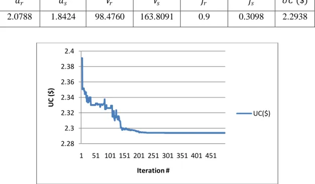
temperature (Constraints 8 and 16) ... 34 Figure 2.6 Unit production cost reduction with respect to the iteration number ... 39 Figure 3.1 The effect of minimum chip thickness (𝑅𝑒 denotes the cutting edge radius,𝑕𝑚 denotes minimum chip thickness and 𝑕 denotes undeformed chip thickness) (Chae et al., 2006) ... 45 Figure 3.2 CCD for three factors ... 52 Figure 3.3 (a) Micro Tools DT-110 (b) Kistler 9256 C1 dynamometer (c) NI PXI-7854R data acquisition card and PC (d) SEM image of micro cutting tool ... 55 Figure 3.4 Cutting tool is plunged out of the workpiece and feed direction is given in (a) and (b). Cutting tool is plunged into the workpiece with small feed rate and feed direction is given in (c) and (d) ... 57 Figure 3.5 Surface roughness measurement of experiment #2: (a) Channel #1 (b) Channel #19 61 Figure 3.6 Micro channel milling force measurements in Exp #2: (a) Channel #1, (b) Channel #9, (c) Channel #19 ... 62

(11)

Figure 3.7 Change in cutting forces ... 63

Figure 3.8 Relationship between tool wear and surface roughness ... 66

Figure 3.9 (a) Linear cutting strategy (b) Spiral cutting strategy ... 68

Figure 3.10 (a) Tool path generated by Cimatron, (b) Actual tool path after machining ... 69

Figure 3.11 As the feed direction changes (a), direction of cutting forces changes (b) ... 72

Figure 3.12 Cutting Forces with respect to axial depth of cuts (a) 80, (b) 114, (c)160 micron ... 74

Figure 3.13 ANOVA result of ∅ 0.8 mm pocket milling experiments ... 75

Figure 3.14 Tool wears of different cutting conditions ... 77

Figure 3.15 Resultant force increase due to tool wear for axial depth of cuts (a) 80 µm, (b) 114 µm and (c) 160 µm ... 79

Figure 3.16 Surface images of first pockets ... 81

Figure 3.17 Surface images of tenth pockets ... 82

Figure 3.18 The effect of cutting conditions in terms of burr formation ... 84

Figure 3.19 Experimental design of ∅ 0.4 mm cutting tool pocket milling experiments ... 87

Figure 3.20 Images of (a) fresh and (b) worn tools ... 89

Figure 3.21 Measured tool diameters values with respect to the number of passes for experiments # 1, #2 and #3 ... 90

Figure 3.22 ANOVA and regression analysis ... 92

Figure 4.1 Tool path from center to outwards ... 95

(12)

LIST OF TABLES

Table 1.1 Guideline for design of experiments (Montgomery, 2004) ... 8

Table 2.1 Particle swarm optimization parameter values ... 24

Table 2.2 Swarm size and iteration number analysis for PSO ... 36

Table 2.3 Acceleration parameter analysis for PSO ... 36

Table 2.4 Unit production cost values obtained in the literature ... 37

Table 2.5 Obtained cutting parameters and UC for a single rough cut and a single finish cut .... 38

Table 2.6 Obtained cutting parameters and UC for two rough cuts and a single finish cut ... 39

Table 2.7 Obtained cutting parameters and UC for a single rough cut and a single finish cut .... 40

Table 2.8 Obtained cutting parameters and UC for two rough cuts and single finish cut ... 40

Table 2.9 Obtained unit costs and CPU times for different initial solutions ... 41

Table 3.1 Controllable factors in experimental studies ... 54

Table 3.2 Slot milling experiment parameters ... 59

Table 3.3 Measurements of slot milling experiments for ∅ 0.8 mm cutting tool ... 60

Table 3.4 Tool life values of experiments 1,2,3 and 4 ... 64

Table 3.5 Slot milling parameters for ∅ 0.4 mm cutting tool ... 65

Table 3.6 Measurements of slot milling experiments for ∅ 0.4 mm cutting tool... 65

Table 3.7 Spindle speed and feed parameters used in ∅ 0.8 mm cutting tool pocket milling experiments... 70

Table 3.8 Axial and radial depth of cut parameters used in ∅ 0.8 mm cutting tool pocket milling experiments... 70

Table 3.9 Tool wear rates of experiment parameters ... 79

(13)

Table 3.11 Determined tool lives for burr formation criteria ... 83

Table 3.12 Measured cutting tool diameter after the preliminary study... 85

Table 3.13 Parameter ranges used in ∅ 0.4 mm cutting tool pocket milling experiments... 86

Table 3.14 Experiment parameters ... 88

Table 3.15 Tool life values obtained in the experiments ... 91

Table 4.1 Tool return and plunge feed rates ... 100

Table 4.2 Obtained results due to tool manufacturer catalogue values ... 101

Table 4.3 Obtained cutting parameters obtained by PSO ... 102

(14)

Chapter 1

Introduction

Manufacturing is defined as transformation of raw materials into finished goods through application of physical and chemical processes. Raw materials follow a sequence of manufacturing operations and as a result finished goods are obtained. The critical issue is to add value in each manufacturing step so that the finished product becomes more valuable than the starting raw material (Groover, 2012). Manufacturing requires machinery, power, labor, know-how and effective use of these is paramount for high value added manufacturing. Minimization of production time, cost and energy while improving the part quality is the main goal in manufacturing.

Globalization, which is defined as the integration and interdependency of world markets in producing consumer goods and services, has immensely impacted manufacturing industry worldwide. As a result of globalization, the rules of competition between developed and emerging nations have changed and consequently the gravity of

(15)

manufacturing industry has been shifted towards Asia. In a recent report, Moavenzadeh et al. (2012) laid out some predictions about the future of global manufacturing based on current economic developments in US and European countries. These can be summarized as:

 It is necessary to invest in infrastructure for high value added manufacturing

 Foreign direct investment is important for the growth of emerging countries and the competition will intensify in near future

 Demand for materials with superior properties (light and durable, rare eath materials, etc.) will grow which will possibly result in breakthroughs in materials sciences

 Affordable clean energy resources will differentiate the competition among developed countries

 Level of human talent will determine the prosperity of countries and companies

Figure 1.1 shows the percentage of manufacturing in gross domestic products (GDP) for various countries. It can be seen from the figure that the percentage of manufacturing has been decreasing for a long period of time whereas the percentage of service industries in the GDP has been rising. This is mainly due to the decrease in relative prices of goods, in conjunction with the simultaneous growth of the demand for services. (Moavenzadeh et al., 2012)

(16)

Figure 1.1 Manufacturing as percent of GDP between 1980 – 2008 (Hunter, 2010)

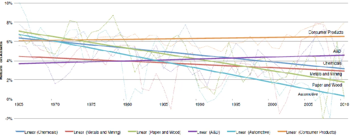
Figure 1.2 shows the historical data of return on assets (ROA) variation for different industries between 1965 and 2010 in USA. Based on the data, only the Aerospace and Defense (A&D) and Consumer Products sectors are on the rise, while the ROA of other manufacturing sectors have been declining since 1965. The most drastic decrease has been observed in labor intensive Automotive Industry which will cease adding value in near future based on the data given in Figure 1.2. It seems like the only way for developed countries to maintain their economic welfare is through innovation which explains their special interest in micro and nano technologies. It is believed that these new technologies will have profound effects on the development of future innovative consumer products.

(17)

Figure 1.2 Shift in manufacturing sectors ROA values in US (Moavenzadeh et al., 2012)

As the manufacturing industry shifts to emerging countries, so does the technological know-how. With the help of existing digital infrastructure (internet, online data storage, etc.), engineers can easily collaborate using computer aided design, engineering, and manufacturing (CAD, CAE, CAM) software even they reside in different countries. This allows faster development products based on customer requirements and reduce the time it takes to introduce the product to the market. Design and manufacturing can be streamlined, if the gaps between CAx tools and computer numerical controlled (CNC) manufacturing processes can be filled within the framework of computer aided process planning (CAPP) systems. As a result, the general objectives of manufacturing can be satisfied.

Figure 1.3 summarizes such efforts in aerospace manufacturing, where the goal is to produce the first-part-correct with minimum trial and error. Computer aided engineering tools, high level automation, physics based process knowledge are integrated from manufacturing planning to quality control of finished parts within a systematic approach. This can only be made possible through a detail oriented investigation of manufacturing

(18)

processes. Similar examples can also be given for other industries such as the production of biomedical and electronics devices.

Figure 1.3 Enabling technologies for high performance manufacturing (Kappmeyer et al., 2012)

A major class in manufacturing processes is the material removal processes. The most important processes in this category are turning, drilling, and milling processes as shown in Figure 1.4.

(19)

Figure 1.4 Material removal processes (Groover, 2012)

These processes use a cutting tool which is harder than the material being shaped in the process. The cutting tools shave off the material from the surface until the desired shape is obtained. A good surface quality can be obtained as a result of machining process. The cutting tool itself also wears out during the process based on the material properties of the tool and the part.

Machining process parameters must be set well in order to obtain an acceptable part quality considering the economics of the process. The cost of manufacturing, the speed of manufacturing and the produced part quality are conflicting objectives hence pose interesting optimization problems. In machining optimization problems, cutting speed, feed, depth of cut etc. are considered as process variables and the goal is to set these process variables to obtain minimum unit cost or maximum productivity (minimum processing time). Figure 1.5 shows the general machining optimization problems for minimum unit cost and maximum productivity cases. As cutting speed increases, machining time decreases which also decrease machining costs. However, tool life decreases as a result of faster processing which increases tooling cost which also means that machine will be idle due to tool change which will further increase total costs. Achieving optimum cutting conditions is important to minimize machining costs in aerospace industry or minimizing machining time in mold making industry.

(20)

Figure 1.5 Machining optimization for minimum cost and maximum productivity (Groover, 2012)

Unfortunately these problems cannot be solved without any experimental data since reliable calculation of process outputs such as tool life and surface quality is not possible. These can only be calculated through experimental methods. Experimentation reveals influential factors that trigger variations in a process/system, to detect most influential factors on the output of a process/system or to find out the most suitable set of factors that minimizes the effect of uncontrollable factors such as noise and develop a robust process/system. Design of experiments (DOE) technique has an important role on generating model of the process/system correctly. In order to generate an accurate model

(21)

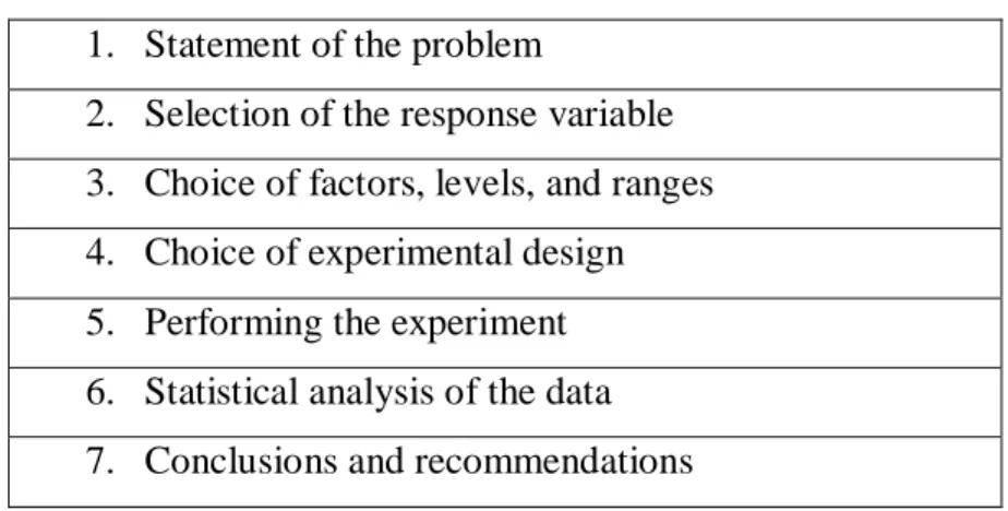
of the physical process, experiment parameters need to be well-chosen since the resulting model depends on the observed data. In manufacturing processes, DOE is widely used to improve the quality of a product, shorten the processing time and increase the life of cutting tool. Table 1.1 shows the outline of the DOE procedure.

Table 1.1 Guideline for design of experiments (Montgomery, 2004) 1. Statement of the problem

2. Selection of the response variable 3. Choice of factors, levels, and ranges 4. Choice of experimental design 5. Performing the experiment 6. Statistical analysis of the data 7. Conclusions and recommendations

It is possible to use regression techniques to represent the data obtained experimentally. Mathematical modeling techniques can be used to obtain the relationship between the objectives as a function of process parameters and various optimization techniques can be used to obtain optimum set of machining parameters. The objective functions in machining problems are usually nonlinear and constrained. As a result, evolutionary optimization algorithms are commonly employed to solve these optimization problems. The approach explained above is used in this thesis, to study macro and micro scale machining optimization problems.

1.1 Motivation

A recent trend in manufacturing industry is towards miniaturization, which has become more important in various industries such as biomedical, consumer products, electronics

(22)

in order to improve the quality of human life by producing more functional products which consume less energy. Micro power generators, fuel cells, lab-on-chip systems, stents, medical screening devices, micro robots and components of cell phones, miniature mold and dies for the mass production of plastic micro parts are some applications. It must be noted that, these are all high value added products and they can be produced in small factories with low energy requirements.

In order to produce miniature products, highly accurate micro components are required. Hence, different types of micromachining processes have been developed and used to produce micro components. Removal by mechanical force (micro milling, turning, drilling), removal by melting, vaporization, and ablation (micro electrical discharge machining, laser machining etc.) are some examples of these processes. Fabrication of micro components necessitates reliable, repeatable, cost effective and fast processes. Although lithography, laser, ion beam and micro EDM methods are available to manufacture good quality micro parts, they are not very preferable because of high costs, material and geometric limitations and time inefficiency. On the other hand, mechanical micromachining is a class of viable micro-manufacturing techniques for producing three dimensional (3D) features on various engineering materials such as metals, composite materials, ceramics and polymers. (Masuzawa, 2000)

Mechanical micromachining has advantages in manufacturing micro components. One of the advantages is that set up and tool costs are not expensive with regard to other techniques. Besides, it is possible to fabricate a broad range of materials with complex 3D geometries such as micro molds. Among mechanical micro manufacturing techniques, micro milling is considered as the most the flexible method. Unlike conventional milling process, the knowledge base for micro milling process is limited.

(23)

The general objective of this study is to contribute to the development of knowledge base for micro milling process. A particular application area is selected as the manufacturing of micro molds. Machining of micro molds can be divided into roughing and finishing processes where the roughing process can be considered as a series of pocketing operations. In this thesis, pocketing operation is investigated in detail and optimization of micro milling process is performed based on the pocketing model developed in this thesis. An evolutionary optimization technique called particle swarm optimization is used to obtain economical machining conditions. The performance of the PSO is also compared with conventional optimization algorithms.

1.2 Organization of the Thesis

The organization of the thesis is detailed below:

In Chapter 2, modeling and optimization of macro scale turning problem is considered. This section is considered as a benchmark study to test the effectiveness of particle swarm optimization (PSO) method against the results given in the literature. In Chapter 3, experimental study conducted on micro milling is explained. Factors affecting micro milling forces, burr formation and surface roughness are explained and tool life expressions for micro milling is obtained. In Chapter 4, mathematical modeling of square pocket milling operation is developed and optimization of the pocketing operation is performed. In Chapter 5, conclusions are drawn and future research directions are given.

(24)

Chapter 2

Modeling and Optimization of

Macro-Scale Turning Operation

Material removal processes are one of the most frequently used methods in manufacturing. Turning, milling and drilling are the most important operations among the material removal processes. This chapter focuses on the process parameter optimization for pass macro-scale turning operation. Firstly, literature on multi-pass macro-scale turning operations is summarized. Secondly, the mathematical formulation of the multi-pass turning operation problem from the literature is explained. Thirdly, Particle Swarm Optimization algorithm is explained. And finally, a numerical example is given in order to test and compare the performance of PSO and nonlinear optimization algorithms with the results reported in the literature.

(25)

2.1 Literature Review on Multi Pass Turning Operation Problem

The main objective of machining operations is fabricating high quality products with low costs in the shortest time. In order to achieve this objective, the selection of the machining parameters, such as cutting speed, depth of cut and feed rate, has become an important issue. Thus, many researchers studied the optimization of process parameter in turning operations.

Gilbert (1950) studied optimization of machining process for single-pass turning operation. Maximum production rate and minimum cost are considered as objective functions and gained different results from each objectives. Ermer (1971) added various operating constraints to the optimization model of single-pass turning operation and used geometric programming.

Shin and Joo (1992) presented an optimization model for multi-pass turning operations. In their study, cutting operations are divided into two parts as rough cutting and finishing cutting, and two sub-problems are solved separately using dynamic programming. Unit production cost is considered as objective function and consists of four main parts which are machining cost, machine idling cost, tool cost and tool replacement cost. Cutting speed, feed rate and axial depth of cut are determined as decision variables. Optimal solutions are obtained for both roughing and finishing operations in this study. Chen and Tsai (1996) modified the multi-pass turning optimization model of Shin and Joo (1992) by adding relation constraints for rough cutting and finishing cutting. Thus, the problem is solved considering both rough and finishing cutting simultaneously instead of solving two sub-problems. The objective of the model is minimizing unit production cost by using rough and finishing cutting speed, rough and finishing feed rate, finishing axial depth of cut and number of rough cutting as decision variables. Simulated Annealing (SA) Algorithm and Hooke-Jeeves Pattern

(26)

Search (SA/HJPS) based optimization algorithm is used to solve the nonlinear optimization problem. It is observed that the algorithm finds near optimal solution set within a reasonable computation time.

Chen (2004) applied scatter search (SS) algorithm to solve the multi-pass turning optimization problem stated by Chen and Tsai (1996). In this study, constrained nonlinear problem is converted into an unconstrained nonlinear problem by adding a penalty function to the objective function instead of defining constraints. An extremely large positive constant is given to the penalty function. Thus, objective function will be extremely large, if one of constraints is violated. The results indicated that scatter search algorithm found better solutions than FEGA and Hooke-Jeeves Pattern Search.

Onwubolu and Kumalo (2001) proposed a new optimization technique based on genetic algorithm (GA) to solve the same model proposed by Chen and Tsai (1996). While the objective function is same with the model constructed by Chen and Tsai (1996), the decision variables are set different from the previous work. Although Onwubolu and Kumalo (2001) obtained better results with respect to Chen and Tsai (1996), their result is invalid since they overlooked total depth of cut equality constraint which stated in the mathematical model of Chen and Tsai (1996). Chen and Chen (2003) realized the mistakes that Onwubolu and Kumalo (2001) made and published the correct results of their work.

Vijayakumar et al. (2003) applied ant colony algorithm (ACO) to solve the multi-pass turning optimization problem presented by Chen and Tsai (1996) and claimed that the proposed ACO algorithm provides better results than previously reported results. Machining parameters, number of passes and depth of cut are determined as decision variables and problem is solved as maximization of negative sign unit production cost. Wang (2007) stated that the solution achieved by Vijayakumar et al. (2003) is also not

(27)

valid. In order to check the validity of optimal solution, unit production cost is computed using the given values of parameters. Since optimal depth of cut information is not given in the study, Wang (2007) tried different number of pass values and revealed that minimum possible objective function value is larger than the result found in Vijayakumar et al (2003).

Yıldız (2009) proposed a hybrid method which combines immune algorithm and hill climbing local search algorithm (HIHC) to solve the nonlinear multi-pass turning optimization problem. The hybrid algorithm combines high exploration speed of immune algorithm with powerful ability of hill climbing local search algorithm to prevent being trapped in local minimum. The same objective function and constraint set of Chen and Tsai (1996) is used in the study. It is revealed that HIHC outperforms FEGA, SA/HJPS and SS. However, the values of parameters found in the achieved solution are not provided. Costa et al. (2011) presented a hybrid particle swarm optimization (HPSO) algorithm to minimize unit production cost in multi-pass turning optimization problem. The hybrid algorithm consists of simulated annealing algorithm to enhance the search mechanism and particle swarm optimization algorithm to move away from local optima. In this study, a similar method to Chen (2004) is used. A penalty function is defined and added to the objective function in order to construct unconstrained nonlinear model instead of solving constrained nonlinear model. Besides, a repair procedure is used to avoid violation in equality constraints. Algorithm is performed for different total depth of cuts. Besides, various comparison modules are done to benchmark with previous works. According to the obtained results, HPSO provides better solutions than the previous works.

(28)

2.2 Mathematical Modeling

The process parameter optimization is done for multiple rough cuts and a single finish cut. The mathematical formulation of multi-pass turning operation model stated in Chen and Tsai (1996) is adopted for the process optimization problem which aims to minimize unit production cost. Unit production cost consists of four basic cost elements. These cost elements are actual machining time cost, machine idling cost due to the loading/unloading operations and idle tool motions, tool replacement cost and tool cost. While searching near optimal machining conditions, technological and physical restrictions are considered. These restrictions are cutting parameter and tool life upper / lower limits, maximum cutting force, machine power and chip-tool interface temperature. Relationship between rough and finish cut, stable cutting region restriction and maximum allowable surface roughness are also considered. In this model, the effect of reduction in workpiece diameter is not taken into consideration. In order to consider the diameter reduction effect, a modified model is also introduced.

The notation used in the mathematical model of multi-pass conventional turning is as follows: 𝑉_𝑟 ∶ 𝑐𝑢𝑡𝑡𝑖𝑛𝑔 𝑠𝑝𝑒𝑒𝑑 𝑖𝑛 𝑟𝑜𝑢𝑔𝑕 𝑚𝑎𝑐𝑕𝑖𝑛𝑖𝑛𝑔 (𝑚 𝑚𝑖𝑛) 𝑉𝑠 ∶ 𝑐𝑢𝑡𝑡𝑖𝑛𝑔 𝑠𝑝𝑒𝑒𝑑 𝑖𝑛 𝑓𝑖𝑛𝑖𝑠𝑕 𝑚𝑎𝑐𝑕𝑖𝑛𝑖𝑛𝑔 (𝑚 𝑚𝑖𝑛) 𝑓𝑟 ∶ 𝑓𝑒𝑒𝑑 𝑟𝑎𝑡𝑒 𝑖𝑛 𝑟𝑜𝑢𝑔𝑕 𝑚𝑎𝑐𝑕𝑖𝑛𝑖𝑛𝑔 (𝑚𝑚 𝑟𝑒𝑣) 𝑓𝑠 ∶ 𝑓𝑒𝑒𝑑 𝑟𝑎𝑡𝑒 𝑖𝑛 𝑓𝑖𝑛𝑖𝑠𝑕 𝑚𝑎𝑐𝑕𝑖𝑛𝑖𝑛𝑔 (𝑚𝑚 𝑟𝑒𝑣) 𝑑𝑠 ∶ 𝑑𝑒𝑝𝑡𝑕 𝑜𝑓 𝑐𝑢𝑡 𝑓𝑜𝑟 𝑒𝑎𝑐𝑕 𝑝𝑎𝑠𝑠 𝑜𝑓 𝑓𝑖𝑛𝑖𝑠𝑕 𝑚𝑎𝑐𝑕𝑖𝑛𝑖𝑛𝑔 (𝑚𝑚) 𝑛 ∶ 𝑛𝑢𝑚𝑏𝑒𝑟 𝑜𝑓 𝑟𝑜𝑢𝑔𝑕 𝑝𝑎𝑠𝑠𝑒𝑠 𝑈𝐶 ∶ 𝑢𝑛𝑖𝑡 𝑝𝑟𝑜𝑑𝑢𝑐𝑡𝑖𝑜𝑛 𝑐𝑜𝑠𝑡 𝑒𝑥𝑐𝑒𝑝𝑡 𝑚𝑎𝑡𝑒𝑟𝑖𝑎𝑙 𝑐𝑜𝑠𝑡 ($ 𝑝𝑖𝑒𝑐𝑒) 𝐶₀∶ 𝑐𝑜𝑛𝑠𝑡𝑎𝑛𝑡 𝑝𝑒𝑟𝑡𝑎𝑖𝑛𝑖𝑛𝑔 𝑡𝑜 𝑡𝑜𝑜𝑙 𝑙𝑖𝑓𝑒 𝑒𝑞𝑢𝑎𝑡𝑖𝑜𝑛 𝐶𝐼∶ 𝑚𝑎𝑐𝑕𝑖𝑛𝑒 𝑖𝑑𝑙𝑒 𝑐𝑜𝑠𝑡 ($ 𝑝𝑖𝑒𝑐𝑒) 𝐶 ∶ 𝑐𝑢𝑡𝑡𝑖𝑛𝑔 𝑐𝑜𝑠𝑡 𝑏𝑦 𝑎𝑐𝑡𝑢𝑎𝑙 𝑡𝑖𝑚𝑒 𝑖𝑛 𝑐𝑢𝑡 ($ 𝑝𝑖𝑒𝑐𝑒)

(29)

𝐶_𝑅∶ 𝑡𝑜𝑜𝑙 𝑟𝑒𝑝𝑙𝑎𝑐𝑒𝑚𝑒𝑛𝑡 𝑐𝑜𝑠𝑡 ($ 𝑝𝑖𝑒𝑐𝑒) 𝐶𝑇 ∶ 𝑡𝑜𝑜𝑙 𝑐𝑜𝑠𝑡 ($ 𝑝𝑖𝑒𝑐𝑒) 𝑑𝑟 ∶ 𝑑𝑒𝑝𝑡𝑕 𝑜𝑓 𝑐𝑢𝑡 𝑓𝑜𝑟 𝑒𝑎𝑐𝑕 𝑝𝑎𝑠𝑠 𝑜𝑓 𝑟𝑜𝑢𝑔𝑕 𝑚𝑎𝑐𝑕𝑖𝑛𝑖𝑛𝑔 (𝑚𝑚) 𝑑𝑡 ∶ 𝑡𝑜𝑡𝑎𝑙 𝑑𝑒𝑝𝑡𝑕 𝑜𝑓 𝑚𝑒𝑡𝑎𝑙 𝑡𝑜 𝑏𝑒 𝑐𝑢𝑡 (𝑚𝑚) 𝑑𝑟𝐿, 𝑑𝑟𝑈 ∶ 𝑙𝑜𝑤𝑒𝑟 𝑎𝑛𝑑 𝑢𝑝𝑝𝑒𝑟 𝑏𝑜𝑢𝑛𝑑𝑠 𝑜𝑓 𝑑𝑒𝑝𝑡𝑕 𝑜𝑓 𝑟𝑜𝑢𝑔𝑕 𝑐𝑢𝑡 (𝑚𝑚) 𝑑_𝑠𝐿, 𝑑_𝑠𝑈 ∶ 𝑙𝑜𝑤𝑒𝑟 𝑎𝑛𝑑 𝑢𝑝𝑝𝑒𝑟 𝑏𝑜𝑢𝑛𝑑𝑠 𝑜𝑓 𝑑𝑒𝑝𝑡𝑕 𝑜𝑓 𝑓𝑖𝑛𝑖𝑠𝑕 𝑐𝑢𝑡 (𝑚𝑚) 𝐷 ∶ 𝑑𝑖𝑎𝑚𝑒𝑡𝑒𝑟 𝑜𝑓 𝑤𝑜𝑟𝑘𝑝𝑖𝑒𝑐𝑒 (𝑚𝑚) 𝑓𝑟𝐿, 𝑓𝑟𝑈 ∶ 𝑙𝑜𝑤𝑒𝑟 𝑎𝑛𝑑 𝑢𝑝𝑝𝑒𝑟 𝑏𝑜𝑢𝑛𝑑𝑠 𝑜𝑓 𝑓𝑒𝑒𝑑 𝑟𝑎𝑡𝑒 𝑖𝑛 𝑟𝑜𝑢𝑔𝑕 𝑐𝑢𝑡 (𝑚𝑚 𝑟𝑒𝑣) 𝑓𝑠𝐿, 𝑓𝑠𝑈 ∶ 𝑙𝑜𝑤𝑒𝑟 𝑎𝑛𝑑 𝑢𝑝𝑝𝑒𝑟 𝑏𝑜𝑢𝑛𝑑𝑠 𝑜𝑓 𝑓𝑒𝑒𝑑 𝑟𝑎𝑡𝑒 𝑖𝑛 𝑓𝑖𝑛𝑖𝑠𝑕 𝑐𝑢𝑡 (𝑚𝑚 𝑟𝑒𝑣) 𝑉_𝑟𝐿, 𝑉_𝑟𝑈 ∶ 𝑙𝑜𝑤𝑒𝑟 𝑎𝑛𝑑 𝑢𝑝𝑝𝑒𝑟 𝑏𝑜𝑢𝑛𝑑𝑠 𝑜𝑓 𝑐𝑢𝑡𝑡𝑖𝑛𝑔 𝑠𝑝𝑒𝑒𝑑 𝑖𝑛 𝑟𝑜𝑢𝑔𝑕 𝑐𝑢𝑡 (𝑚 𝑚𝑖𝑛) 𝑉𝑠𝐿, 𝑉𝑠𝑈 ∶ 𝑙𝑜𝑤𝑒𝑟 𝑎𝑛𝑑 𝑢𝑝𝑝𝑒𝑟 𝑏𝑜𝑢𝑛𝑑𝑠 𝑜𝑓 𝑐𝑢𝑡𝑡𝑖𝑛𝑔 𝑠𝑝𝑒𝑒𝑑 𝑖𝑛 𝑓𝑖𝑛𝑖𝑠𝑕 𝑐𝑢𝑡 (𝑚 𝑚𝑖𝑛) 𝐹𝑟, 𝐹𝑠 ∶ 𝑐𝑢𝑡𝑡𝑖𝑛𝑔 𝑓𝑜𝑟𝑐𝑒𝑠 𝑑𝑢𝑟𝑖𝑛𝑔 𝑟𝑜𝑢𝑔𝑕 𝑎𝑛𝑑 𝑓𝑖𝑛𝑖𝑠𝑕 𝑐𝑢𝑡𝑡𝑖𝑛𝑔 (𝑘𝑔 𝑓) 𝐹_𝑈 ∶ 𝑚𝑎𝑥𝑖𝑚𝑢𝑚 𝑎𝑙𝑙𝑜𝑤𝑎𝑏𝑙𝑒 𝑐𝑢𝑡𝑡𝑖𝑛𝑔 𝑓𝑜𝑟𝑐𝑒 (𝑘𝑔 𝑓) 𝑕1, 𝑕2∶ 𝑐𝑜𝑛𝑠𝑡𝑎𝑛𝑡𝑠 𝑝𝑒𝑟𝑡𝑎𝑖𝑛𝑖𝑛𝑔 𝑡𝑜 𝑡𝑜𝑜𝑙 𝑡𝑟𝑎𝑣𝑒𝑙 𝑎𝑛𝑑 𝑎𝑝𝑝𝑟𝑜𝑎𝑐𝑕, 𝑑𝑒𝑝𝑎𝑟𝑡 𝑡𝑖𝑚𝑒 (𝑚𝑖𝑛) 𝑘₁, 𝑘₂, 𝑘₃ ∶ 𝑐𝑜𝑛𝑠𝑡𝑎𝑛𝑡𝑠 𝑓𝑜𝑟 𝑟𝑜𝑢𝑔𝑕𝑖𝑛𝑔 𝑎𝑛𝑑 𝑓𝑖𝑛𝑖𝑠𝑕𝑖𝑛𝑔 𝑝𝑎𝑟𝑎𝑚𝑒𝑡𝑒𝑟 𝑟𝑒𝑙𝑎𝑡𝑖𝑜𝑛𝑠 𝑘_𝑓 ∶ 𝑐𝑜𝑒𝑓𝑓𝑖𝑐𝑖𝑒𝑛𝑡 𝑝𝑒𝑟𝑡𝑎𝑖𝑛𝑖𝑛𝑔 𝑡𝑜 𝑠𝑝𝑒𝑐𝑖𝑓𝑖𝑐 𝑡𝑜𝑜𝑙 − 𝑤𝑜𝑟𝑘𝑝𝑖𝑒𝑐𝑒 𝑐𝑜𝑚𝑏𝑖𝑛𝑎𝑡𝑖𝑜𝑛 𝑘₀∶ 𝑑𝑖𝑟𝑒𝑐𝑡 𝑙𝑎𝑏𝑜𝑟 𝑜𝑣𝑒𝑟𝑕𝑒𝑎𝑑 𝑐𝑜𝑠𝑡 ($ 𝑚𝑖𝑛) 𝑘_𝑞 ∶ 𝑐𝑜𝑒𝑓𝑓𝑖𝑐𝑖𝑒𝑛𝑡 𝑝𝑒𝑟𝑡𝑎𝑖𝑛𝑖𝑛𝑔 𝑡𝑜 𝑒𝑞𝑢𝑎𝑡𝑖𝑜𝑛 𝑜𝑓 𝑡𝑜𝑜𝑙 − 𝑐𝑕𝑖𝑝 𝑖𝑛𝑡𝑒𝑟𝑓𝑎𝑐𝑒 𝑡𝑒𝑚𝑝𝑒𝑟𝑎𝑡𝑢𝑟𝑒 𝑘_𝑡 ∶ 𝑐𝑢𝑡𝑡𝑖𝑛𝑔 𝑒𝑑𝑔𝑒 𝑐𝑜𝑠𝑡 ($ 𝑒𝑑𝑔𝑒) 𝐿 ∶ 𝑙𝑒𝑛𝑔𝑡𝑕 𝑜𝑓 𝑤𝑜𝑟𝑘𝑝𝑖𝑒𝑐𝑒 (𝑚𝑚) 𝑝, 𝑞, 𝑟 ∶ 𝑐𝑜𝑛𝑠𝑡𝑎𝑛𝑡𝑠 𝑝𝑒𝑟𝑡𝑎𝑖𝑛𝑖𝑛𝑔 𝑡𝑜 𝑡𝑕𝑒 𝑡𝑜𝑜𝑙 − 𝑙𝑖𝑓𝑒 𝑒𝑞𝑢𝑎𝑡𝑖𝑜𝑛 𝑃_𝑟, 𝑃_𝑠 ∶ 𝑐𝑢𝑡𝑡𝑖𝑛𝑔 𝑝𝑜𝑤𝑒𝑟𝑠 𝑑𝑢𝑟𝑖𝑛𝑔 𝑟𝑜𝑢𝑔𝑕 𝑎𝑛𝑑 𝑓𝑖𝑛𝑖𝑠𝑕 𝑐𝑢𝑡𝑡𝑖𝑛𝑔 (𝑘𝑊) 𝑃_𝑈 ∶ 𝑚𝑎𝑥𝑖𝑚𝑢𝑚 𝑎𝑙𝑙𝑜𝑤𝑎𝑏𝑙𝑒 𝑐𝑢𝑡𝑡𝑖𝑛𝑔 𝑝𝑜𝑤𝑒𝑟 (𝑘𝑊) 𝑄_𝑟, 𝑄_𝑠 ∶ 𝑡𝑒𝑚𝑝𝑒𝑟𝑎𝑡𝑢𝑟𝑒𝑠 𝑑𝑢𝑟𝑖𝑛𝑔 𝑟𝑜𝑢𝑔𝑕 𝑎𝑛𝑑 𝑓𝑖𝑛𝑖𝑠𝑕 𝑐𝑢𝑡𝑡𝑖𝑛𝑔 (˚𝐶) 𝑄_𝑈 ∶ 𝑚𝑎𝑥𝑖𝑚𝑢𝑚 𝑎𝑙𝑙𝑜𝑤𝑎𝑏𝑙𝑒 𝑡𝑒𝑚𝑝𝑒𝑟𝑎𝑡𝑢𝑟𝑒 (˚𝐶) 𝑅_𝑎 ∶ 𝑚𝑎𝑥𝑖𝑚𝑢𝑚 𝑎𝑙𝑙𝑜𝑤𝑎𝑏𝑙𝑒 𝑠𝑢𝑟𝑓𝑎𝑐𝑒 𝑟𝑜𝑢𝑔𝑕𝑛𝑒𝑠𝑠 (µ𝑚) 𝑅_𝑛 ∶ 𝑛𝑜𝑠𝑒 𝑟𝑎𝑑𝑖𝑢𝑠 𝑜𝑓 𝑐𝑢𝑡𝑡𝑖𝑛𝑔 𝑡𝑜𝑜𝑙 (𝑚𝑚) 𝑆_𝑐 ∶ 𝑙𝑖𝑚𝑖𝑡 𝑜𝑓 𝑠𝑡𝑎𝑏𝑙𝑒 𝑐𝑢𝑡𝑡𝑖𝑛𝑔 𝑟𝑒𝑔𝑖𝑜𝑛 𝑡 ∶ 𝑡𝑜𝑜𝑙 𝑙𝑖𝑓𝑒 (min) 𝑡 ∶ 𝑐𝑜𝑛𝑠𝑡𝑎𝑛𝑡 𝑡𝑒𝑟𝑚 𝑜𝑓 𝑚𝑎𝑐𝑕𝑖𝑛𝑒 𝑖𝑑𝑙𝑖𝑛𝑔 𝑡𝑖𝑚𝑒 (min)

(30)

𝑡_𝑒 ∶ 𝑡𝑜𝑜𝑙 𝑒𝑥𝑐𝑕𝑎𝑛𝑔𝑒 𝑡𝑖𝑚𝑒 (min) 𝑡_𝑝 ∶ 𝑡𝑜𝑜𝑙 𝑙𝑖𝑓𝑒 min 𝑐𝑜𝑛𝑠𝑖𝑑𝑒𝑟𝑖𝑛𝑔 𝑟𝑜𝑢𝑔𝑕𝑖𝑛𝑔 𝑎𝑛𝑑 𝑓𝑖𝑛𝑖𝑠𝑕𝑖𝑛𝑔 𝑡𝑟, 𝑡𝑠 ∶ 𝑡𝑜𝑜𝑙 𝑙𝑖𝑣𝑒𝑠 min 𝑐𝑜𝑛𝑠𝑖𝑑𝑒𝑟𝑖𝑛𝑔 𝑟𝑜𝑢𝑔𝑕𝑖𝑛𝑔 𝑎𝑛𝑑 𝑓𝑖𝑛𝑖𝑠𝑕𝑖𝑛𝑔 𝑡𝑣 ∶ 𝑣𝑎𝑟𝑖𝑎𝑏𝑙𝑒 𝑡𝑒𝑟𝑚 𝑜𝑓 𝑚𝑎𝑐𝑕𝑖𝑛𝑒 𝑖𝑑𝑙𝑖𝑛𝑔 𝑡𝑖𝑚𝑒 min 𝑇_𝐼∶ 𝑚𝑎𝑐𝑕𝑖𝑛𝑒 𝑖𝑑𝑙𝑖𝑛𝑔 𝑡𝑖𝑚𝑒 min 𝑇𝐿, 𝑇𝑈 ∶ 𝑙𝑜𝑤𝑒𝑟 𝑎𝑛𝑑 𝑢𝑝𝑝𝑒𝑟 𝑏𝑜𝑢𝑛𝑑 𝑜𝑓 𝑡𝑜𝑜𝑙 𝑙𝑖𝑓𝑒 min 𝑇𝑀 ∶ 𝑐𝑢𝑡𝑡𝑖𝑛𝑔 𝑡𝑖𝑚𝑒 𝑏𝑦 𝑎𝑐𝑡𝑢𝑎𝑙 𝑚𝑎𝑐𝑕𝑖𝑛𝑖𝑛𝑔 min 𝑇𝑀𝑟, 𝑇𝑀𝑠 ∶ 𝑐𝑢𝑡𝑡𝑖𝑛𝑔 𝑡𝑖𝑚𝑒 𝑏𝑦 𝑎𝑐𝑡𝑢𝑎𝑙 𝑚𝑎𝑐𝑕𝑖𝑛𝑖𝑛𝑔 𝑓𝑜𝑟 𝑟𝑜𝑢𝑔𝑕𝑖𝑛𝑔 𝑎𝑛𝑑 𝑓𝑖𝑛𝑖𝑠𝑕𝑖𝑛𝑔 min 𝑇_𝑅 ∶ 𝑡𝑜𝑜𝑙 𝑟𝑒𝑝𝑙𝑎𝑐𝑒𝑚𝑒𝑛𝑡 𝑡𝑖𝑚𝑒 min 𝑋 ∶ 𝑣𝑒𝑐𝑡𝑜𝑟 𝑜𝑓 𝑐𝑢𝑡𝑡𝑖𝑛𝑔 𝑝𝑎𝑟𝑎𝑚𝑒𝑡𝑒𝑟𝑠 𝜏, 𝜙, 𝛿 ∶ 𝑐𝑜𝑛𝑠𝑡𝑎𝑛𝑡𝑠 𝑝𝑒𝑟𝑡𝑎𝑖𝑛𝑖𝑛𝑔 𝑡𝑜 𝑒𝑥𝑝𝑟𝑒𝑠𝑠𝑖𝑜𝑛 𝑜𝑓 𝑐𝑕𝑖𝑝 𝑡𝑜𝑜𝑙 𝑖𝑛𝑡𝑒𝑟𝑓𝑎𝑐𝑒 𝑡𝑒𝑚𝑝𝑒𝑟𝑎𝑡𝑢𝑟𝑒 𝜂 ∶ 𝑝𝑜𝑤𝑒𝑟 𝑒𝑓𝑓𝑖𝑐𝑖𝑒𝑛𝑐𝑦 𝜆, 𝜈 ∶ 𝑐𝑜𝑛𝑠𝑡𝑎𝑛𝑡𝑠 𝑝𝑒𝑟𝑡𝑎𝑖𝑛𝑖𝑛𝑔 𝑡𝑜 𝑒𝑥𝑝𝑟𝑒𝑠𝑠𝑖𝑜𝑛 𝑜𝑓 𝑠𝑡𝑎𝑏𝑙𝑒 𝑐𝑢𝑡𝑡𝑖𝑛𝑔 𝑟𝑒𝑔𝑖𝑜𝑛 𝜇, 𝜐 ∶ 𝑐𝑜𝑛𝑠𝑡𝑎𝑛𝑡𝑠 𝑜𝑓 𝑐𝑢𝑡𝑡𝑖𝑛𝑔 𝑓𝑜𝑟𝑐𝑒 𝑒𝑞𝑢𝑎𝑡𝑖𝑜𝑛 𝜃 ∶ 𝑎 𝑤𝑒𝑖𝑔𝑕𝑡 𝑓𝑜𝑟 𝑡𝑝 𝑤𝑕𝑒𝑟𝑒 0 < 𝜃 < 1

As a first case, the mathematical model formulated by Chen and Tsai (1996), which neglects the effect of workpiece diameter reduction on unit production cost, is solved. The mathematical model of the first case is given as following:

min 𝑈𝐶 = 𝐶𝑀 + 𝐶𝐼+ 𝐶𝑅+ 𝐶𝑇 subject to 𝑑_𝑟𝐿 ≤ 𝑑_𝑟 ≤ 𝑑_𝑟𝑈 (1) 𝑓_𝑟𝐿 ≤ 𝑓_𝑟 ≤ 𝑓_𝑟𝑈 (2) 𝑉𝑟𝐿 ≤ 𝑉𝑟 ≤ 𝑉𝑟𝑈 (3) 𝑇_𝐿 ≤ 𝑡_𝑟 ≤ 𝑇_𝑈 (4) 𝑘_𝑓𝑓_𝑟𝜇𝑑_𝑟𝜐 _{≤ 𝐹} 𝑈 (5)

(31)

𝑘𝑓𝑓𝑟𝜇𝑑𝑟𝜐𝑉𝑟 6120 𝜂 ≤ 𝑃𝑈 (6) 𝑉_𝑟𝜆_𝑓 𝑟𝑑𝑟𝜈 ≥ 𝑆𝑐 (7) 𝑘_𝑞𝑉_𝑟𝜏_𝑓 𝑟𝜙𝑑𝑟𝛿 ≤ 𝑄𝑈 (8) 𝑑_𝑠𝐿 ≤ 𝑑_𝑠 ≤ 𝑑_𝑠𝑈 (9) 𝑓𝑠𝐿 ≤ 𝑓𝑠 ≤ 𝑓𝑠𝑈 (10) 𝑉_𝑠𝐿 ≤ 𝑉_𝑠 ≤ 𝑉_𝑠𝑈 (11) 𝑇_𝐿 ≤ 𝑡_𝑠 ≤ 𝑇_𝑈 (12) 𝑘_𝑓𝑓_𝑠𝜇𝑑_𝑠𝜐 _{≤ 𝐹} 𝑈 (13) 𝑘𝑓𝑓𝑠𝜇𝑑𝑠𝜐𝑉𝑠 6120 𝜂 ≤ 𝑃𝑈 (14) 𝑉𝑠𝜆𝑓𝑠𝑑𝑠𝜈 ≥ 𝑆𝑐 (15) 𝑘_𝑞𝑉_𝑠𝜏_𝑓 𝑠𝜙𝑑𝑠𝛿 ≤ 𝑄𝑈 (16) 𝑓𝑠2 8𝑅𝑛 ≤ 𝑅𝑎 (17) 𝑉_𝑠 ≥ 𝑘₁𝑉_𝑟 (18) 𝑓_𝑟 ≥ 𝑘₂𝑓_𝑠 (19) 𝑑𝑟 ≥ 𝑘3𝑑𝑠 (20) 𝑑_𝑟 = (𝑑_𝑡 − 𝑑_𝑠) 𝑛 (21)

In the model, 𝑉_𝑟, 𝑓_𝑟, 𝑉_𝑠, 𝑓_𝑠, 𝑛 𝑎𝑛𝑑 𝑑_𝑠 are determined as the decision variables.

Unit production cost (𝑈𝐶) is calculated as the sum of four basic cost elements which are 𝐶_𝑀, 𝐶_𝐼, 𝐶_𝑅, 𝐶_𝑇. The formulation of each cost element is as follows:

𝐶_𝑀 = 𝑘₀𝑇_𝑀 (22) 𝐶𝐼 = 𝑘0 𝑡𝑐 + 𝑕1𝐿 + 𝑕2 (𝑛 + 1) (23)

𝐶_𝑅 = 𝑘₀𝑡𝑒

(32)

𝐶_𝑇 = 𝑘𝑡 𝑡𝑝 𝑇𝑀 (25) where 𝑇𝑀= 𝑛𝑇𝑀𝑟+ 𝑇𝑀𝑠 (26) 𝑇𝑀𝑟 = _{1000 𝑉}𝜋𝐷𝐿 𝑟𝑓𝑟 (27) 𝑇𝑀𝑠 =_{1000 𝑉}𝜋𝐷𝐿 𝑠𝑓𝑠 (28)

Actual machining cost (𝐶𝑀) is divided into two components which are multiple roughing

and single finishing costs. Machine idling cost (𝐶_𝐼) has two constant terms, loading and unloading operation costs and a variable term idle motion time due to tool motions between passes and length of workpiece. In tool replacement cost (𝐶_𝑅) calculation, it is assumed that a single tool can be used for both rough cut and finish cut operations. Thus, the tool life is calculated as following:

𝑡_𝑝 = 𝜃𝑡_𝑟+ (1 − 𝜃)𝑡_𝑠 (29) where 𝑡_𝑟 = 𝐶0 𝑉_𝑟𝑝𝑓_𝑟𝑞𝑑𝑟𝑟 (30) 𝑡_𝑠 = 𝐶0 𝑉_𝑠𝑝𝑓_𝑠𝑞𝑑𝑠𝑟 (31)

In order to estimate tool replacement cost, required number of tools and tool changing time are used. Tool cost (𝐶_𝑇) is calculated by considering number of used tools.

Constraints (1), (2) and (3) bound depth of cut, feed rate and cutting speed for roughing process respectively. Constraint (4) keeps roughing process tool life within an

(33)

acceptable range to manufacture economic and high quality products. Constraint (5), (6) and (8) restrict the cutting force, power and chip – tool interface temperatures in the course of roughing operations. Constraint (7) ensures the cutting conditions of roughing process stay in the stable region. Constraints (9), (10) and (11) guarantee that the depth of cut, feed rate and cutting speed bounds for finish cut are not terminated. Constraint (12) keeps finishing process tool life within the determined range. Constraint (13), (14) and (16) restricts the cutting force, power and chip – tool interface temperatures during the finishing operations respectively. Constraint (15) ensures the cutting conditions of finish cut stay in the stable region. Constraint (17) provides that the quality of machined surface is within the required range. Constraints (18) – (20) define the relations of cutting speed, feed rate and depth of cut in roughing and finishing processes. Constraint (21) ensures that total depth of cut is equal to the sum of finishing depth of cut and total depth of roughing cut.

It must be noted that the diameter of the workpiece is assumed to be fixed during the cutting process in the original formulation. This may be a valid assumption if the diameter reduction is assumed to be small. Cutting speed is kept constant during the turning process which means that the rotational speed of the spindle must be increased as diameter decreases which implies that feed rate must increase at each pass therefore machining time changes in every machining pass. Decrease in part diameter affects unit production cost. For analyzing the effect of decrease in part diameter, another case is created. A modification is applied to the objective function of Chen and Tsai (1996) as a second case in order to investigate the effect of decrease in workpiece diameter on unit cost by considering the same restrictions. The diameter information is updated at each pass. In the second case, actual machining time of rough cut (𝑇_𝑀𝑟) and finish cut (𝑇_𝑀𝑠) are reformulated with respect to the assumption. Machining time calculation method is as follows:

(34)

1𝑠𝑡_{𝑟𝑜𝑢𝑔𝑕 𝑝𝑎𝑠𝑠 ∶} 𝜋𝐷𝐿 1000 𝑉𝑟𝑓𝑟 (32) 2𝑛𝑑_{𝑟𝑜𝑢𝑔𝑕 𝑝𝑎𝑠𝑠 ∶}𝜋(𝐷−2𝑑𝑟)𝐿 1000 𝑉𝑟𝑓𝑟 (33) 𝑛𝑡𝑕_{𝑟𝑜𝑢𝑔𝑕 𝑝𝑎𝑠𝑠 ∶}𝜋 (𝐷−2(𝑛−1)𝑑𝑟)𝐿 1000 𝑉𝑟𝑓𝑟 (34) 𝑓𝑖𝑛𝑖𝑠𝑕 𝑝𝑎𝑠𝑠 ∶ 𝜋(𝐷−𝑛𝑑𝑟)𝐿 1000 𝑉𝑠𝑓𝑠 (35)

Objective function of the second case is as follows:

min 𝑈𝐶 = 𝐶_𝑀+ 𝐶_𝐼+ 𝐶_𝑅+ 𝐶_𝑇 where 𝐶_𝑀 = 𝑘₀ 𝜋(𝐷−2𝑖𝑑𝑟)𝐿 1000 𝑉𝑟𝑓𝑟 𝑛−1 𝑖=0 +𝜋(𝐷−2𝑛𝑑_{1000 𝑉}_𝑠_𝑓𝑟_𝑠)𝐿 (36) 𝐶_𝐼 = 𝑘₀ 𝑡_𝑐+ 𝑕₁𝐿 + 𝑕₂ (𝑛 + 1) (37) 𝐶𝑅 = 𝑘0_𝑡𝑡𝑒 𝑝 𝜋(𝐷−2𝑖𝑑𝑟)𝐿 1000 𝑉𝑟𝑓𝑟 𝑛−1 𝑖=0 +𝜋 (𝐷−2𝑛𝑑_{1000 𝑉}_𝑠_𝑓𝑟_𝑠)𝐿 (38) 𝐶_𝑇 = 𝑘𝑡 𝑡𝑝 𝜋(𝐷−2𝑖𝑑𝑟)𝐿 1000 𝑉𝑟𝑓𝑟 𝑛−1 𝑖=0 +𝜋(𝐷−2𝑛𝑑_{1000 𝑉}_𝑠_𝑓𝑟_𝑠)𝐿 (39)

𝐶𝐼 is not affected from the modification since the terms in machine idling cost is not

dependent on actual machining time. However, machining time formulation of 𝐶_𝑀, 𝐶_𝑅 and 𝐶_𝑇 are changed due to the new assumption. Decision variables and constraints remain same as the first case.

As mentioned earlier, PSO is used to solve the multi pass turning optimization problem. PSO technique is explained in the next section.

(35)

2.3 Particle Swarm Optimization (PSO)

Particle Swarm Optimization (PSO) algorithms have been used in various optimization problems ranging from simple problems to highly complex problems. It has become a popular method in handling machining process optimization problems due to its robustness and efficiency. PSO is developed by Kennedy and Eberhart (1995). It is a population based stochastic optimization method inspired from the social behaviors of animals or insects such as bird flocking and fish schooling.

In PSO, a population of particles is randomly scattered in the search space. Each particle in the swarm has its own path in the search space. The path is updated by using its previous position information and current velocity at each iteration. The dimensions of position and velocity vectors are determined due to the number of decision variables in the model. As the solution improved, search space is narrowed around the highest performing particle for detailed search. The process continues until reaching the termination criteria.

In the algorithm, the velocity of each particle is updated by considering best position found by the particle (𝑝𝑏𝑒𝑠𝑡) and best position found by the entire population (𝑔𝑏𝑒𝑠𝑡). The update procedure is done with respect to the following equations:

𝑣_𝑖𝑘 +1 _{= 𝑤𝑣}

𝑖𝑘 + 𝑐1𝑟1 𝑝𝑏𝑒𝑠𝑡𝑖 − 𝑥𝑖𝑘 + 𝑐2𝑟2 𝑔𝑏𝑒𝑠𝑡 − 𝑥𝑖𝑘 (40)

𝑥_𝑖𝑘+1 _{= 𝑥}

𝑖𝑘 + 𝑣𝑖𝑘+1 (41)

where 𝑣_𝑖𝑘 denotes velocity of particle 𝑖 at iteration 𝑘, 𝑥_𝑖𝑘 denotes current position of particle 𝑖 at iteration 𝑘, 𝑝𝑏𝑒𝑠𝑡_𝑖 denotes personal best position of particle 𝑖, 𝑔𝑏𝑒𝑠𝑡 denotes the best position in the entire population, 𝑟₁ and 𝑟₂ denote random values

(36)

generated between 0 and 1, 𝑐₁ and 𝑐₂ denote acceleration coefficients and 𝑤 denotes the inertia weight.

Equation (40) shows the update procedure of velocity. It consists of three different terms. The first term 𝑤𝑣_𝑖𝑘 is the weighted ratio of particle velocity and is used to carry the particle in its previous direction. The second term 𝑐₁𝑟₁ 𝑝𝑏𝑒𝑠𝑡_𝑖 − 𝑥_𝑖𝑘_{is used to carry}

the information of particles best position. The last term 𝑐₂𝑟₂ 𝑔𝑏𝑒𝑠𝑡 − 𝑥_𝑖𝑘 attracts the entire population to the particle which performs best in the swarm. Random numbers 𝑟₁ and 𝑟₂ are used to provide stochastic behavior to the algorithm. Inertia weight 𝑤 is used to define the area of search space. The algorithm searches a wide space when the inertia weight is large. Large inertia weight is commonly used at the beginning of the algorithm. As the solution improved, inertia weight can be reduced in order to confine the search region near 𝑔𝑏𝑒𝑠𝑡.

Equation (41) shows the update procedure of particles’ current position. The position of particle is updated by using the velocity update term. The procedure of PSO is summarized as follows:

Step 1: Generate initial population with its positions and velocities.

Step 2: Evaluate the objective function of all particles. Assign the current position of

each particle and its objective function value as 𝑝𝑏𝑒𝑠𝑡. Select the best solution within the entire population and assign as 𝑔𝑏𝑒𝑠𝑡.

Step 3: Generate new positions and velocities of particles. If a particle has a better

(37)

Evaluate each particles’ 𝑝𝑏𝑒𝑠𝑡 value and assign 𝑔𝑏𝑒𝑠𝑡. If the new 𝑔𝑏𝑒𝑠𝑡 is better than the previous 𝑔𝑏𝑒𝑠𝑡 value, update 𝑔𝑏𝑒𝑠𝑡 value.

Step 4: Repeat step 2 and step 3 until reaching determined iteration number.

Karpat and Özel (2006) developed a neural network model to model the surface roughness and tool wear characteristics of CBN tools and used particle swarm optimization (PSO) to optimize cutting parameters of turning operations. Karpat and Özel (2007) used multi objective particle swarm optimization (MOPSO) method in order to optimize hard turning operation for the cases of tool life and material removal rate maximization and surface roughness and machining time minimization. A Pareto optimal set is obtained for multi objective optimization problem.

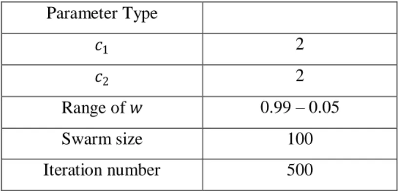
Parameter selection has an important role on the processing time and solution quality of the heuristic algorithms. Thus, an analysis is required in order to increase the speed of algorithm without losing the solution quality. Parameter analysis is performed for the particle swarm optimization algorithm and the determined parameter values are given in Table 2.1. The detailed analysis of parameter selection is given in the numerical study section.

Table 2.1 Particle swarm optimization parameter values Parameter Type 𝑐₁ 2 𝑐₂ 2 Range of 𝑤 0.99 – 0.05 Swarm size 100 Iteration number 500

(38)

2.4 Numerical Study

In this section, a numerical study is performed to analyze the effects of decision variables on the model, determine particle swarm optimization algorithm parameters, evaluate and compare the performance of PSO with the results given in the literature. All of the analyses are performed on a personal computer with 2.20 GHz Intel Core 2 Duo CPU and 2 GB of RAM.

The constraints of cutting force, power, stable region and chip-tool interface temperature are investigated in order to measure the effects of decision variables on the model. Parameters of PSO are fine tuned using the turning operation model of Chen and Tsai (1996) and the data which is presented in Figure 2.1. For algorithm evaluation, the results obtained through PSO are compared with the previous studies. Besides, Matlab Optimization Toolbox which uses trust region, active set or interior point algorithms is also included in the comparison. The data used in the computational study is given in Figure 2.1.

(39)

2.4.1 Constraint Analysis of Mathematical Model

Prior to the evaluation of PSO performance, the effects of decision variables on cutting force, power, stability and chip-tool interface constraints are investigated. Since the bounds in both roughing and finishing operation parameters and the constraint equations are the same, analysis is done with respect to three decision variables which are cutting speed, feed rate and depth of cut. In order to visualize the effects, three dimensional surface plots are created.

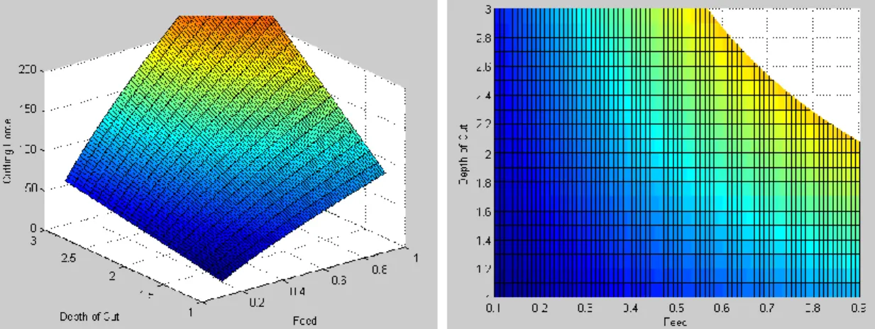
In Figure 2.2, the effects of feed rate and depth of cut on cutting force are introduced. It is revealed from the figure that cutting force increases as the depth of cut and feed rate increases. High feed rate and depth of cut values induce infeasibility in the problem. The white area in part (b) represents the infeasible region for cutting force constraints.

(a) (b)

Figure 2.2 Effects of feed rate and depth of cut on cutting force (Constraints 5 and 13)

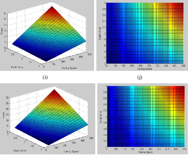
In Figure 2.3, the effects of feed rate, depth of cut and cutting speed on machine power are presented. Since there are three decision variables that affect power constraint, it is not possible to investigate the effect of all variables on power simultaneously. Thus,

(40)

these variables are divided into groups of two and all possible combinations are analyzed. While constructing the groups, the remaining decision variable is fixed at its lower and upper bounds separately. In parts (a) – (b) and (c) – (d), the effects of depth of cut and feed rate are explored by fixing the cutting speed to its lower limit and upper limit respectively. In parts (e) – (f) and (g) – (h), the effects of cutting speed and feed rate are analyzed by fixing the depth of cut to its lower limit and upper limit respectively. In parts (i) – (j) and (k) – (l), the effects of depth of cut and cutting speed are searched by fixing the feed rate to its lower limit and upper limit respectively. Due to the surface plots, machine power increases by increasing depth of cut, feed rate and cutting speed. When the differences of highest obtained power values for lower and upper limits of the fixed decision variables are investigated, it is discovered that cutting speed changes the power value most. The second effective decision variable is feed rate and third effective is depth of cut.

(41)

(c) (d)

(e) (f)

(42)

(i) (j)

(k) (l)

Figure 2.3 Effects of cutting speed, depth of cut and feed rate on power (Constraints 6 and 14)

Besides, power constraint is never terminated within the given ranges of cutting speed, depth of cut and feed rate. Although the upper limit of power is 200 kW, the maximum obtained power is 27.24 kW.

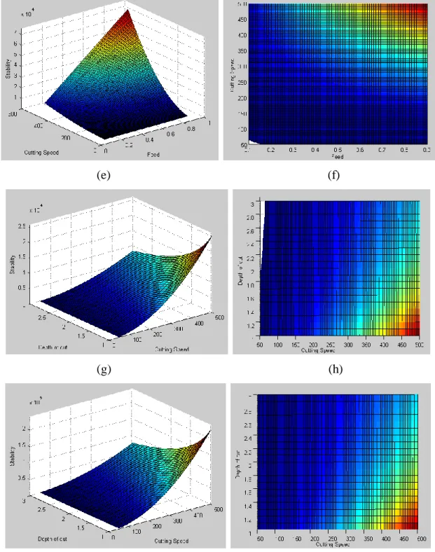
In Figure 2.4, the effects of feed rate, depth of cut and cutting speed on stable region are shown. The same methodology with power constraint analysis is used in the course of the investigation of decision variables on stability constraint. In parts (a) – (b), the effects of depth of cut and feed rate are explored by fixing the cutting speed to its lower

(43)

limit. The cutting speed is also fixed to the upper limit. However, feasible region for the fixed upper limit of cutting speed does not exist. In parts (c) – (d) and (e) – (f), the effects of cutting speed and feed rate are analyzed by fixing the depth of cut to its lower limit and upper limit respectively. In parts (g) – (h) and (i) – (j), the effects of depth of cut and cutting speed are searched by fixing the feed rate to its lower limit and upper limit respectively. It is revealed from the analysis that depth of cut should be small. If the depth of cut needs to be increased, feed rate and cutting speed should be increased in order to stay in the stable cutting region. Besides, stability cannot be achieved for the upper limit of cutting speed.

(a) (b)

(44)

(e) (f)

(g) (h)

(i) (j)

(45)

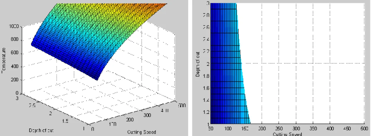
In Figure 2.5, the effects of feed rate, depth of cut and cutting speed on chip-tool interface temperature are presented. Since the effect of three decision variables on temperature cannot be visualized in one plot, the same approach with power and stable region analysis is used. In parts (a) – (b), the effects of depth of cut and feed rate are explored by fixing the cutting speed to its lower limit. Analysis is done for the upper limit, but feasible region cannot be found. In parts (c) – (d) and (e) – (f), the effects of cutting speed and feed rate are analyzed by fixing the depth of cut to its lower limit and upper limit respectively. In parts (g) – (h) and (i) – (j), the effects of depth of cut and cutting speed are searched by fixing the feed rate to its lower limit and upper limit respectively.

(46)

(c) (d)

(e) (f)

(47)

(i) (j)

Figure 2.5 Effects of cutting speed, depth of cut and feed rate on chip – tool interface temperature (Constraints 8 and 16)

Due to the analysis, the most effective variable on chip – tool interface temperature is cutting speed. While all feed rate and depth of cut values are feasible for lower limit of cutting speed, feasible region cannot be found for the upper limit of cutting speed. It is also revealed that the effect of feed rate on temperature is more than the depth of cut. In order to reduce the temperature on chip – tool interface, cutting speed, feed rate, and depth of cut should also be decreased. It is revealed from these analyses that the most restrictive constraint is stable region constraint. Besides, power constraint is never terminated within the given range. The effects of decision variables change with respect to the constraint type.

2.4.2 Parameter Analysis of Particle Swarm Optimization

Fine-tuning of algorithm parameter is an important task since the parameters affect the convergence of algorithm. The inertia weight adjusts the trade-off between the local and global exploration capability of the swarm. Large inertia weight is used to search wide areas while small inertia weight is used to search narrow areas. It is beneficial to select a

(48)

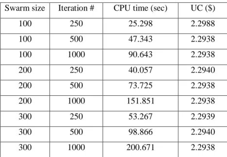
large inertia weight at the beginning of the algorithm in order to scatter particles in the feasible region. As the number of iteration increases, the inertia weight should be reduced to focus the search on a narrow area around the global best particle. Thus, inertia weight is selected as 0.99 initially. Then, it is gradually declined towards 0.05 for detailed search. The acceleration parameters 𝑐₁ and 𝑐₂ determine the speed of convergence. Kennedy (1998) proposed 𝑐₁ = 𝑐₂ = 2 as default values. For 𝑐₁ = 𝑐₂ = 2 and 𝑤 = 0.99 − 0.05 values, the impact of swarm size and iteration number for termination is investigated. The result obtained from the analysis is given in Table 2.2. Due to the results, the minimum unit cost obtained in this study is $2.2938 and the result is achieved by most of the parameter sets. However, minimum cost with minimum CPU time is obtained with swarm size of 100 and iteration number of 500. Thus, swarm size and terminating iteration number for PSO is selected as 100 and 500 respectively. After determining the swarm size and termination criteria, the effect of change in acceleration parameters are investigated. In Table 2.3, the result of acceleration parameter is shown. According to the results, the values proposed by Kennedy (1998) are the best values for this optimization problem. Hence, acceleration coefficients are fixed to the value of 2, interval of inertia weight is determined as 0.99 – 0.05, population size is set to 100 and the algorithm is terminated after 500 iterations.

(49)

Table 2.2 Swarm size and iteration number analysis for PSO Swarm size Iteration # CPU time (sec) UC ($)

100 250 25.298 2.2988 100 500 47.343 2.2938 100 1000 90.643 2.2938 200 250 40.057 2.2940 200 500 73.725 2.2938 200 1000 151.851 2.2938 300 250 53.267 2.2939 300 500 98.866 2.2940 300 1000 200.671 2.2938

Table 2.3 Acceleration parameter analysis for PSO

𝑐1 𝑐2 CPU Time (sec) UC ($)

0.5 2 49.091 2.3154 1 2 53.841 2.2941 1.5 2 51.887 2.2940 2 2 47.343 2.2938 2 1.5 50.322 2.2939 2 1 49.874 2.2938 2 0.5 47.702 2.2938 1 1 47.415 2.2938

(50)

2.4.3 Performance Evaluation of Particle Swarm Optimization

Macro-scale turning operation is one of the most frequently used operation type in machining processes. The model formulated by Chen and Tsai (1998) is solved by many researchers using different heuristic methods for the same parameter set. Table 2.4 summarizes the obtained results in the previous studies.

Table 2.4 Unit production cost values obtained in the literature

Study Method 𝑈𝐶

Chen and Tsai (1996) SA / HJPS $ 2.2959

Onwubolu,Kumalo (2001) Genetic Algorithm $ 1.7610

Chen and Chen (2003) FEGA $ 2.3065

Viyajakumar (2003) ACO $ 1.6262

Chen (2004) SS $ 2.0667

Wang (2007) Correction to Viyajakumar $ 2.5429

Yıldız (2009) HIHC $ 2.0468

Costa et al. (2011) HPSO $ 1.9591

Chen and Tsai (1996) used SA / HJPS method. All of the constraints given in mathematical modeling section are considered in the constrained nonlinear model. The obtained unit production cost in this study is $2.2959. Onwubolu and Kumalo (2001) introduced a new optimization technique based on GA. Although all constraints are taken into account in this study, number of rough cuts is not limited to an integer. Thus, unit production cost of $1.761 is not a valid result. Chen and Chen (2003) revealed the mistake in Onwubolu and Kumalo (2001) and mentioned that the solution is infeasible due to the constraint violation. In addition, they applied FEGA method to solve the same model and reached the result of $2.3065 per unit. Viyajakumar (2003) proposed ACO to

(51)

obtain near optimal values of multi-pass conventional turning machine parameters. In this study, achieved parameters are not provided. They stated that unit production cost per piece is $1.6262. Chen (2004) proposed SS method in order to solve the benchmark problem. Constraints (1) – (21) are used in this study. The best result obtained in this study is $2.0667. However, the values of the decision variables are not provided. Wang (2007) analyzed the cutting parameters that are found in Viyajakumar (2003) and stated that unit production cost cannot be gained with the provided decision variable values. With respect to Wang (2007), the minimum possible unit production cost is $1.968 for one rough cut and $2.5429 for two rough cuts. Yıldız (2009) solved multi-pass conventional turning optimization model in order to evaluate the performance of HIHC method. The whole constraint set given in mathematical modeling section is considered in the model. According to the gained result, minimum unit production cost is $2.0468. The machining parameters are not provided in the study. Costa et al. (2011) used HPSO method and provided different benchmark models in order to compare the efficiency of HPSO with respect to other proposed studies. For different comparison models, various results are obtained. It is mentioned in the study that minimum unit productions cost obtained by HPSO is $1.9591, but cutting parameters are not provided.

Mathematical model of the first case is solved for two different alternatives using PSO. The assumption in the first alternative is that, machining operation is done with a single rough cut and a single finish cut. Under this assumption, objective function value and its cutting conditions are given in Table 2.5.

Table 2.5 Obtained cutting parameters and UC for a single rough cut and a single finish cut

𝑑𝑟 𝑑𝑠 𝑉𝑟 𝑉𝑠 𝑓𝑟 𝑓𝑠 𝑈𝐶 ($)