YAŞAR UNIVERSITY
GRADUATE SCHOOL OF NATURAL AND APPLIED SCIENCES MASTER THESIS
WAVELET BASED HARMONIC ANALYSIS: CASE
STUDY OF A PLANT WITH COGENERATION
Güneş BECERİK
Thesis Advisor: Asst. Prof. Hacer ŞEKERCİ
Department of Electric and Electronic Engineering
Presentation Date: 28.10.2015
Bornova-İZMİR 2015
iii
ABSTRACT
WAVELET BASED HARMONIC ANALYSIS: CASE STUDY OF A PLANT WITH COGENERATION
BECERİK, Güneş
MSc in Electrical and Electronic Engineering Supervisor: Asst. Prof. Hacer ŞEKERCİ ÖZTURA
October 2015, 67 pages
Industrial countries constitute energy policies in order to decrease energy gap and minimize environmental issues. Increasing use of renewable energy sources and with the expansion of using distributed generation is the solutions to energy related problems in our country. A cogeneration system is a distribution generation unit which supplies electrical and heat demand of the developing industry. These systems are more preferable due to its higher efficiencies against separate generation systems and lower environmental impact. The cogeneration system which analyzed in this thesis is installed in İzmir and fed 3 different loads. It connects to interconnection point via point common coupling which can be used in case the cogeneration switches to island mode.
In the first part of this study, the harmonic components of different operating modes of a cogeneration system are analyzed. Since wavelet based algorithm tracks harmonics effectively and gives in time frequency spectrum, the wavelet theory is used among the methods covered in literature to find harmonics. Studies have been conducted to choose a mother wavelet. This analysis is aimed to determine the direction of harmonic flow on both gas turbines and loads. In the second part, low-pass filters and de-noising algorithm are used to decrease the effect of harmonics. It is observed that wavelet based global thresholding decrease harmonics effectively.
In the last part of the study; comparisons are made between designed low-pass filter and de-noising algorithm with wavelets. Depending on the selected mother wavelet, de-noising algorithm is found to be quite successful when eliminating harmonics
iv
ÖZET
DALGACIK TABANLI HARMONİK ANALİZİ: KOJENERASYON SİSTEMLİ BİR ÖRNEK OLAY İNCELEMESİ
Güneş BECERİK
Yüksek Lisans Elektrik-Elektronik Mühendisliği Bölümü Tez Danışmanı: Yrd. Doç. Dr. Hacer ŞEKERCİ ÖZTURA
Ekim 2015, 67 sayfa
Sanayi ülkelerinde enerji açığını azaltmak ve çevresel sorunları en aza indirgemek amacıyla çeşitli enerji politikaları oluşturulmaktadır. Yenilenebilir enerji kaynaklarının kullanımının arttırılması ve ayrık üretim sistemlerinin yaygınlaştırılması ile ülkemizde ve dünyada yaşanan enerji sorununa çözüm bulunmaya çalışılmıştır. Bir ayrık üretim sistemi olan kojenerasyon sistemleri gelişmekte olan endüstrinin hem elektrik hem de ısıl ihtiyacını karşılamaktadır. Bu sistemlerin bağımsız olarak ısı ve elektrik üreten tesislere göre daha yüksek verime sahip olması ve çevresel etkilerinin az olması kojenerasyon sistemlerini tercih edilir hale getirmiştir. Bu tezde analiz edilen kojenerasyon sistemi İzmir’de kurulmuş olup; 3 adet yükü beslemektedir. Kuplaj noktası ile enterkonnekte sisteme bağlanarak; gerektiği durumlarda kendini ada durumuna alabilmektedir.
Bu çalışmanın birinci kısmında bir kojenerasyon sistemindeki çeşitli çalışma modlarındaki harmonikler incelenmiştir. Harmonikleri belirlemek için literatürde kullanılan yöntemler içerisinden dalgacık metodu kullanılmıştır. Ana dalgacık seçebilmesi için gerekli çalışmalar yapılmıştır. Dalgacık tabanlı algoritma harmonikleri hızlı bir şekilde tespit ederek frekans zaman spektrumunda vermektedir. Bu analiz, hem türbinler hem de yükler üzerinde gerçekleştirilerek harmoniklerin akış yönünün belirlenmesi amaçlamıştır. Çalışmanın ikinci kısmında ise harmoniklerin etkisini azaltmak için alçak geçirgen filtre ile gürültü süzme algoritması kullanılmıştır. Evrensel eşikleme yöntemi ile harmonikler azaltılarak çıkış sinyali neredeyse giriş sinyaline yaklaşmış; bu şekilde harmoniklerin elenmesi sağlanmıştır.
Çalışmanın son kısmında; Tasarlanan alçak geçirgen filtre ile gürültü süzme algoritması arasında karşılaştırma yapılmıştır. Seçilen ana dalgacığa bağlı olarak
v
gürültü süzme algoritmasının sistem harmoniklerini eleme konusunda oldukça başarılı olduğu gözlenmiştir.
Anahtar sözcükler: Dalgacık analizi, güç sistemlerinde harmonik, evrensel
vi
ACKNOWLEDGEMENTS
I would like to express my sincere gratitude to my supervisor Asst. Prof. Hacer Şekerci for the useful comments, remarks and engagement through the learning process of this master thesis. Furthermore I would like to thank Asst. Prof. Nalan Özkurt for introducing me to the concept of wavelet as well as for the unlimited support on the way. Additionally, I would like to thank Assoc. Prof. Mustafa Seçmen who helped me throughout the coding process.I can't express how much I've learned, grown, and enjoyed working with all of you.
I would also like to thank Ahmet Özenir and Okan Tunç, who have willingly shared their precious time during this survey. Without their support, it is impossible for me to finish this thesis.
Finally, I would like to thank my loved ones, who have supported me throughout entire process, helping me putting pieces together. Last but not the least important, I owe more than thanks to my family members for their endless support and encouragement throughout my life.
vii
TEXT OF OATH
I declare and honestly confirm that my study, titled “Wavelet Based Harmonic Analysis: Case Study of a Plant With Cogeneration” and presented as a Master’s thesis, has been written without applying to any assistance inconsistent with scientific ethics and traditions, that all sources from which I have benefited are listed in the bibliography, and that I have benefited from these sources by means of making references.
viii TABLE OF CONTENTS Page ABSTRACT iii ÖZET iv ACKNOWLEDGEMENTS vi
TEXT OF OATH vii
TABLE OF CONTENTS viii
INDEX OF FIGURES x
INDEX OF TABLES xiii
INDEX OF SYMBOLS AND ABBREVIATIONS xiv
1 INTRODUCTION 0
2 COMBINED HEAT AND POWER 2
2.1 Classification of Cogeneration Systems 3
2.2 Operating Modes of Cogeneration 6
3 WAVELET ANALYSIS 8
3.1 Related Studies 9
3.2 Definition of wavelet 11
ix
3.4 Continuous Wavelet Transform (CWT) 13
3.5 Wavelet Denoising 13
4 METHODOLOGY 20
4.1 Definition of the Plant 20
4.2 Harmonic Analysis 23
Mother Wavelet Selection 24
Harmonic Analysis on Raw data 26
4.3 Filtering and de-noising 31
5 CONCLUSION 40 5.1 FUTURE WORK 41 REFERENCES 42 APPENDIX A 47 APPENDIX B 49 CURRICULUM VITEA 50
x
INDEX OF FIGURES
Figure 2.1 Comparison of energy conservation of cogeneration and separate
generation of electricity and heat (Smit, 2006) ... 2
Figure 2.2 Combined cycle power plant ... 4
Figure 2.3 Diagram of bottoming cycle in CHP (Center for Sustainable Energy, 2015) ... 5
Figure 2.4 Diagram of topping cycle in CHP (Center for Sustainable Energy, 2015) . 5 Figure 2.5 Peak shaving mode ... 6
Figure 3.1 Evolution of wavelet analysis ... 11
Figure 3.4 Schematic diagram wavelet de-noising: multilevel decomposition, thresholding, and multilevel reconstruction. Thresholding is obtained via (a) soft threshold or (b) hard threshold (Aymerich,2014) ... 14
Figure 3.5 DWT decomposition for 1D signal ... 16
Figure 3.6 DWT reconstruction for 1D signal ... 16
Figure 3.7 Visualization of hard and soft thresholding ... 17
Figure 3.2 Description of “cmor0.5-10” and “shan0.5-10... 18
Figure 3.3 Description of Daubechies wavelet with 6 coefficients “db6” ... 19
Figure 4.1 Gas turbine based cogeneration system ... 20
Figure 4.2 Voltage specifications for all customers ... 21
xi
Figure 4.4 Complex Shannon wavelet analysis ... 25
Figure 4.5 Complex Gaussian wavelet analysis ... 25
Figure 4.6 Diagram of the cogeneration plant ... 26
Figure 4.7 Customer-1 current ... 27
Figure 4.8 Fourier spectrum and Scalogram of customer-1 (a) Fourier Spectrum (b) Scalogram ... 28
Figure 4.9 Customer-2 current ... 29
Figure 4.10 Fourier spectrum and Scalogram of customer-2 (a) Fourier Spectrum (b) Scalogram ... 29
Figure 4.11 Customer-3 current (baseload) ... 30
Figure 4.12 Fourier spectrum and Scalogram of customer-2 (a) Fourier Spectrum (b) Scalogram ... 30
Figure 4.13 MATLAB filter design and analysis tool ... 31
Figure 4.14 Low-pass filter specification ... 32
Figure 4.15 Magnitude response of low-pass filter ... 33
Figure 4.16 Customer-1 filtered harmonics ... 35
Figure 4.17 Customer-1 de-noised harmonics ... 35
Figure 4.18 Customer-3 filtered harmonics ... 36
Figure 4.19 Customer-3 de-noised harmonics ... 36
xii
xiii
INDEX OF TABLES
Table 2.1 CHP base technologies ... 3
xiv
INDEX OF SYMBOLS AND ABBREVIATIONS
Symbols Explanations
C Cycle Time (min)
w(t) Window function
x(t) Signal to be analyzed
a Dilation coefficient
b Translation coefficient
𝜓𝑎,𝑏(𝑡) Dilated and translated mother wavelet
w(a) Weighting function
y(i) Noisy signal
𝜀(𝑖) Independently normal random variables Tm,n Detailed wavelet coefficients
ϕ(t) Father wavelet
y Signal after threshold
Threshold valuexv Abbreviations
DG Distributed generation
CHP Combined heat and power
FT Fourier transform
STFT Short time Fourier transform
DWT Discrete Wavelet transform
MRA Multi-resolution analysis
PCC Point common coupling
UPS Uninterruptable Power Supply
0
1 INTRODUCTION
European Union sets a target that utilization on renewable energy is increased 20% by 2020. The predominance of this energy will be obtained by distributed generation units. “Distributed generation, on-site generation or decentralized generation is a term describing the production of electricity for use on-site, rather than transmitting energy over the electric grid from a large centralized facility.” (Environmental and Energy Study Institute, 2015). Energy efficiency increase significantly when electricity is produced smaller amounts and closer to end-users. It is also reduce carbon pollutions and improve quality of the energy.
Distributed generation (DG) can be used to generate entire electricity supply; for peak shaving; stand-by generation or as a green power source. It is used in many areas such as domestic, commercial, industrial and greenhouses. Generation capacity is ranged from few kilowatts to megawatts. Flexibility, reliability and power quality response make these systems more preferable. It has lower capital costs against big generation systems because of its smaller sizes. It increases power reliability as a back-up or stand-by power system. It lowers the need for large constructions and upgrades in present systems. It is also produce near-zero pollutant emissions with some new technologies like biomass. In a combined heat and power application DG efficiencies rise up to 90% because waste heat can be captured and used to generate electricity. (EPCOR, 2015)
Beside of all these benefits there are some challenges associated with DG systems. DG systems are connected to distribution networks. National standards for interconnection and contractual barriers are not clear for these technologies. They have many requirements for fees and charges. Environmental regulations and larger DG systems make these projects uneconomical. The connection of DG causes some issues because distribution system is designed to feed power from a relatively few large station generations. It is not designed to accept the feed in of energy at medium and low voltage levels. Voltage control and balancing, stability and power quality issues, network protection are the important parts that have to be taken into account. (Chapman et al.,2008)
Subject of this thesis contains a study of harmonic analysis and a performance analysis between low-pass filter and wavelet de-noising algorithm. Power system
1
harmonics has a great deal of attention recently. Harmonic identification has an important role in industrial energy audit. Harmonics are primarily due to non-linear loads. Mainly it causes power system resonance so awareness of harmonic issues can help to increase plant power system reliability.
The aim of this thesis is to determine the harmonics and define which customer supply it to the system. All raw data’s are recorded in the same cogeneration plant which consist 3 different customers. Timeline of the data is organized with respect to operating modes such as island mode, base load and low power mode and high power mode. Harmonic analysis is done by using wavelet ridge algorithm. Response of this algorithm shows frequency-amplitude based plot for identifying harmonics. After this analysis, a comparison is made by a FIR low-pass filter and de-noising algorithm. Low pass filter is designed by using MATLAB. For different cases filter is tested and results compared with de-noising response.
A detailed literature search will be given that including the studies are done recently. The details of the methods and selection of the mother wavelet will be explained in the thesis. Methods will be explained while obtaining filtering and de-noising process will be presented for eliminating harmonic components. Applications and result are also demonstrated with graphs and tables for frequency amplitude representations and daily data will be also shown. All results and graphical data’s are presented and the work planned for the future will be discussed briefly.
Structure of the thesis consist 5 chapters. In chapter 2, combined heat and power, classifications, operating modes are represented. In chapter 3, methodology of the thesis which consist wavelet, Fourier analysis, filter theory and de-noising algorithm is presented. In chapter 4, application of harmonic analysis and harmonic filter design is presented and tested in raw data’s. In chapter 5 conclusions, author recommendations for future work will explained. Finally, references, appendix and curriculum vitae are presented.
2
2 COMBINED HEAT AND POWER
Combined heat and power (CHP) or cogeneration is the simultaneous production of power and heat from a single fuel source. It is important that both products have a practical application area. The power product of CHP is electricity but the depending on the cogeneration technology heat product is used for indirectly producing steam, hot water or chilled water for process cooling. (Smit, 2006)
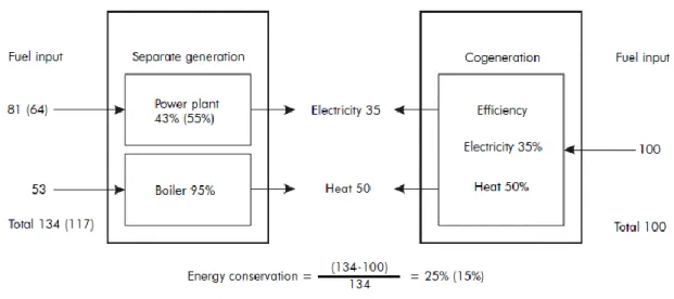
CHP technologies are more efficient than separate heat and power production. Efficiency calculation of electricity generation is determined by the relationship between net electricity and the fuel consumption. Heat rate is represented by consumed fuel per kWh of electricity generated. Total efficiency in CHP system is much higher than the separate generation. Figure 2.1 indicates the energy conservation on both separate generation and a cogeneration unit. A CHP system produces 85 units of useful energy through the conventional generation or separate heat and power systems use 134 units of energy, 64 for electricity production and 53 to produce heat. Overall efficiency is 63 percent. However, the CHP system needs only 100 units of energy to produce the 85 units of useful energy from a single fuel source, resulting in a total system efficiency of 85 percent.
Figure 2.1 Comparison of energy conservation of cogeneration and separate generation of
electricity and heat (Smit,2006)
A system planner must consider several factors when building a cogeneration plant. The most important factor is the stable and predictable heat demand. Heat demand must always greater than the electricity demand. Cogeneration has high
3
initial cost relative to traditional power generation technologies. Energy market conditions and financial resources like prices, feed-in, tax reliefs must be stated and used in feasibility analysis. Proper place for installation is another factor because it requires significant amount of space in a plant.
2.1 Classification of Cogeneration Systems
CHP systems consist of number elements such as heat engine, generator, heat recovery and electrical interconnection. Primarily, classifications of these systems are implemented by using their prime movers. Prime mover technologies are listed in Table 2.1 with respect to power range, electrical and overall efficiencies are indicated (Knowles, 2011).
Table 2.1 CHP base technologies CHP power generation technology Power range (applied to CHP) Power efficiency range (%) CHP efficiency (peak) (%) Steam turbine 500 kW – 100 MW 15 - 40 75 Gas turbine 2 MW – 500 MW 20 - 45 80
Combined cycle gas and
steam turbine 20 MW – 600 MW 30 - 55 85
Reciprocating engine 5 kW – 10 MW 25 - 40 95
Micro turbine 30 kW – 250 kW 25-30 75
Fuel cell 5 kW – 1 MW 30-40 75
Stirling Engine 1 kW – 50 kW 10-25 80
The oldest prime mover technology is based on steam turbines. Steam turbines are mostly used where the demand for electricity is greater than one megawatt. Steam turbine cogeneration system has 2 types: backpressure or extraction/condensing. They replaced with reciprocating steam engines due to higher efficiencies and lower costs. The choices between these two turbines are related to power and heat quantity as well as economic factors. Gas turbine cogeneration systems can produce all electricity requirement of a site and energy released from the exhaust gases can be used by a heat recovery unit. Range of gas turbines varies from
4
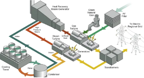
2 MW to 500 MW and natural gas is the most common fuel used in combustion. These systems are highly efficient because of short start up time and flexibility in many operations. It has low heat to power ratio so that more heat can be recovered at higher temperatures. On the other hand if more power is needed in the site, it is possible to combine a gas turbine with a steam turbine to create a combined cycle. It can be seen in figure 2.2 in a combined cycle plant, fuel (natural gas) and air is mixed and ignited in the combustor. Then released gases blast through gas turbine blades and causing them to rotate. An alternator converts this mechanical energy into electrical energy. Produced electricity is transformed into high voltage by using transformers and sent to transmission network. Gas turbines also produce exhaust gases. Steam generated from the exhaust gases passed through a steam turbine to generate additional power. The exhaust or the extracted steam from the steam turbine provides thermal energy.
Figure 2.2 Combined cycle power plant
Micro-turbines are small, radial flow gas turbine. Reciprocating engine also known as internal combustion engines are used in cogeneration units. These units have high power generation capacity in comparison with the others. Heat is recovered from high temperature exhaust gas and engine jacket cooling water system. These systems are preferred when the electricity demand is higher than the thermal demand. (India Bureau of Energy Efficiency, 2004)
5
A cogeneration system can be also classified by the sequence of energy use. This basis divided into two groups as bottoming cycle and topping cycle. figure 2.3 depicted, in the bottoming cycle fuel produces thermal energy and waste heat is used to generate power through a recovery boiler and a turbine generator. Prime movers for bottoming cycle are organic Rankine cycle turbine and steam turbine.
Figure 2.3 Diagram of bottoming cycle in CHP (Center for Sustainable Energy, 2015)
Figure 2.4 shows the working principle of topping cycle. In the topping cycle, fuel is initially used to produce power then thermal energy. Thermal energy is used to satisfy process heat or other thermal requirements. Prime movers for topping cycle are internal combustion engine, gas turbine, micro turbine, fuel cell technologies.
Figure 2.4 Diagram of topping cycle in CHP (Center for Sustainable Energy, 2015)
There are four different types of topping cycle for cogeneration systems. A gas turbine or diesel engine system with a heat recovery boiler creates a combined cycle topping system. Engine or turbine provides electrical/mechanical power and the boiler provides steam to drive a steam turbine. The second type burns any type of fuel and produce high pressure steam to produce electricity from steam turbine. Steam turbine is also produce low pressure steam to use in the process. This is called a steam turbine topping system. The third type operates heat recovery from engine exhaust and/or jacket cooling system. Product of this type converted into steam or hot
6
water. Lastly for the fourth type and the cogeneration unit which is used in this thesis; is a natural gas fueled gas turbine drives a generator. The exhaust gas goes to heat recovery boiler to make steam and process heat. (India Bureau of Energy Efficiency, 2004)
2.2 Operating Modes of Cogeneration
A cogeneration system can operate in many different modes. In parallel grid mode, cogeneration unit works continuously to ensure the electrical demand for the system. Rating of prime mover extends to full of its availability. Plants operating in parallel grid both import and export surplus power to the local distribution network. If electrical demand exceeds its limits, the unit only imports excess power from the grid. This is also called “base-load operation”. A base-load system can also be sized by using thermal loads. If the system is inadequate for the demand supplemental power purchase may be required.
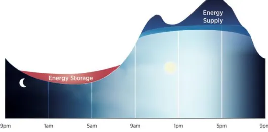
In case of limited capacity it is beneficial to import certain agreed amount of power from the grid and produce excess power with own power generating equipment. This is called “peak-shaving mode”. Figure 2.5 shows the peak shaving operation that can be done by using an energy storage system. The storage system is charged at night (in red) when the system load is low, and then discharged during the day when the system load peaks. This helps reduce the customer’s peak demand cost. (OpenEI, 2015)
7
A cogeneration unit can operate independently from local electricity distribution network. This is called “island mode”. The site is not connected with the utility; it may necessary to install redundant capacity to overcome unscheduled outages. This may be done by increasing the capacity or basically doing a load shedding. Load shedding can helps the system to be served at a certain capacity. Island mode operations can be seen on two forms. Stand-alone generators generate electricity when there is no connection between the plant and electricity grid. Also, if the plant is in parallel grid any failure in network lowers the generator to island mode.
Load tracking mode can be expressed in which the prime movers output is reduced when the site’s energy requirements drop below the prime movers baseload output. Cogeneration system can be operating in load tracking if the engine output is supply the electrical requirements of the site. As in thermal tracking, prime mover is operated in a way so that no heat is rejected.
Final operating mode is economic dispatch mode where the system is operating during the hours when the cost of producing electricity is less than cost of purchased power. If a cogeneration system selling power to an electric utility it is recommended to operate in economic dispatch mode. (Zor ve Teke, 2013; OpenEI, 2015)
8
3 WAVELET ANALYSIS
As it seems a new method in signal processing, wavelet analysis dates back to the work of Joseph Fourier in the 19th century. Frequency based analysis have some limitations and the attention of researchers turned to scale based analysis. The first mention of wavelet is in 1909, in a thesis by Alfred Haar and many scientists made contributions in definition of wavelets, methods of wavelet transform and multiresolution framework.
“Joseph Fourier shows any periodic function can be expressed as an infinite sum of periodic exponential functions.” Fourier transform (FT) tells whether a frequency component exist or not but it does not give any time information due to transforming into frequency domain. If the signal properties do not change in time which is called stationary signals, time information is not important. However, many of the signals are non-stationary or transitory characteristics. Fourier analysis is not suitable for detecting these important characteristics. (Polikar,2001)
Fourier transfrom is very sensitive to changes in the function. A small change can effect entire fourier coefficients. Location of frequency componenets are stored in phases and it is difficult to extract. If a function has Fourier coefficients all have the same magnitude, Fourier transform of this function is focused at a single point. Because of this, it is difficult to determine whether a signal includes a particular frequency at a certain point. (Lambers, 2008) Due to this limitations of FT a new technique is needed for non-stationary signal analysis so windowing technique is discovered by Dennis Gabor. This method provides a window function to analyze a small part of the signal at a time. This adaption is called Short time Fourier transform (STFT). It represents a signal with respect to time-frequency base. Main idea of STFT is to assume some portion of the non-stationary signal is stationary. If this area is too small, then we choose a narrow window to analyze the frequency components. Analyzed signal is divided into segments and multiplied with the window function “w(t)”. For every multiplication STFT coefficients are calculated. Result of these calculations show frequency components for each time interval. It may be seen that STFT is suitable for frequency analysis; but there are some problems. Main drawbacks comes from the width of the window function. If we use a window with infinite length we get the frequency components but there is no time information just like Fourier transform. On the other hand, if we choose a narrow window we have a
9
good time resolution but poor frequency resoultion. All these obstacles lead to researchers for a scaled based analysis of “Wavelet”. (Misiti et al.,2009)
3.1 Related Studies
In this part of the study, publications which used for the harmonic analysis, mother wavelet selection and de-noising techniques are examined. While examining publications, this study focused on wavelet based methods for all sections of the literature.
The advantages of using wavelet transform in harmonic analysis gives better resolution because of the scaled base. It provides distribution of energy with respect frequency sub-bands. A signal can be decomposed into uniform frequency bands and it can be easy to extract detailed information by using wavelet transform. Appropriate selection of sampling frequency spectral leakage is reduced. Meyer and Mallat's theorem (1989) says that given an orthogonal MRA we can find a function whose dilates and translates will create an orthonormal basis. (Pereyra, C.,2015) They develop the Multiresolution analysis (MRA) with using wavelets, which made it practical for engineering applications. MRA is wavelet based discrete filters used in signal processing. Ribeiro (1994) was the first to apply wavelet transform for analyzing nonstationary signals in power systems. The author presents the main concepts of the wavelet theory and application areas of distortion. Santoso et al. (1994) proposed an approach using wavelets to detect and localize electric power quality incidences based on time-scale domain. The authors proposed mother wavelet selection such as db4, db6 is chosen for the case of fast transients and db8 and db10 for the case of slow transients. Pham and Wong (1999) develop a novel approach based on wavelet transform. Proposed algorithm uses continuous wavelet transform to identify all frequency spectrum which includes harmonics and integer/non-integer sub-harmonics. Pham and Wong (2001) also present a method for eliminating the effect of imperfect frequency response of the filters in wavelet transform. Method recovers the signal magnitude by using wavelet based algorithm to give true harmonic amplitudes. Proposed method is used for the diagnosis of a motor-starting problem, which occurred in the Western Australia power system. Chen (2008) presented a multi-resolution wavelet method with 7 levels of reconstructing through db24 to decompose the harmonics. By experiment analysis on MATLAB, error is less than 1% which gives the tracking accuracy effectively. Gu et al. (2011) and Apetrei et
10
al. (2014) used discrete wavelet packet transform to decompose a waveform, and then based on wavelet coefficients harmonic contents are defined. All frequency contents with amplitudes and phases are calculated by continuous wavelet transform.
The choice of mother wavelet is a key parameter in wavelet transform. There are many case studies of choosing the best mother wavelet for harmonic analysis; but there is no agreement for the most suitable one. In the study of harmonic distortion in power system, Tse (2006) and Jing (2010) use ‘Morlet wavelet’ for estimation of the harmonics and inter-harmonics. Morsi and El-Hawary (2008) proposed a method on selection of mother wavelet which based on the energy of wavelet coefficients. Authors have found that the most suitable mother wavelet is ‘Daubechies (db)’ and the accuracy of the analysis increases with increasing wavelet order. For the high distortion level authors propose ‘Coiflet wavelet’ with low order gives accurate results. Kashyap and Singh (2008) made a statistical approach for finding suitable mother wavelet. They compare the performance of different mother wavelets on computation of the root mean square value by using DWT. Authors have found that the most suitable mother wavelet for analyzing harmonics is ‘Daubechies with 7 coefficients (db7)’. Srivasta et al. (2009) made a case study on selection of mother wavelet for the power system harmonics using CWT. In their study, they compare the results with IEEE standard 1459-2000. Performance metrics for the analysis contains two methods: lowest root mean square error and minimum percentage error. It has found that ‘Gaussian wavelet’ is supported for the most suitable wavelet.
Wavelet de-noising removes the noise present in the original signal with optimal balancing and smoothing. It is not confused with smoothing process. Smoothing removes high frequency and retains low frequency components of the signal. DWT based de-noising process aims to remove low frequency contents of the signal. First application is done by Donoho and Johnstone (1995). Author proposed a method which based on thresholds DWT of the signal. Wavelet coefficients are reduced to zero if their values are below to zero. Lang and Guo (1996) also present a similar study for de-noising process. Wavelet threshold is used for de-noising power quality disturbances for classification. Giaouris et al. (2008) propose the use of wavelet transform to extract and identify specific frequency components. Authors presented a pseudo-adaptive de-noising method based on wavelets which adjust level of decomposition depending on the rotor speed. Wavelets are used for high frequency injection. Jie, (2009) detects and locates disturbing points based on soft and hard
11
threshold methods. On the basis author presented a new threshold function according to power quality signal characteristic. Proposed method is better for realization and noising effect. Joy et al. (2013) made a comparative study of different wavelet de-noising techniques. Discrete wavelet transform is done by using multiresolution analysis and digital filters. Through the analysis ‘Daubechies wavelet with 4 coefficients (db4)’ is used as mother wavelet. Authors have found that ‘rigrsure’ method gives the optimum performance. Performance metric is based on SNR and mean square error values. Gupta and Sharma (2015) create a power system model to generate voltage and current signals. White Gaussian noise is added in the input voltage to get a noisy signal. For the analysis wavelet packet tool is used and ‘symentic family (sym)’ is selected as the mother wavelet.
3.2 Definition of wavelet and wavelet families
“A wavelet is a waveform of effectively limited duration that has an average value of zero.” (Arulmozhi and Nadarajan, 2003) Unlike a sine wave, wavelet has a limited time duration, asymmetric and irregular characteristic. Wavelet analysis is primarily explained as a windowing technique with variable-sized windows. Shannon’s time domain representation is evolve and develepod as a scale based representation with the wavelet analysis. Evolution of this technique is demonstrate in figure 3.1
Figure 3.1 Evolution of wavelet analysis
Fourier analysis breaks up the signal into sine waves but wavelet analysis divide signal into shifted and scaled version of the original wavelet. This is called as
12
“mother wavelet”. Wavelet analysis transforms time domain signals into time-frequency domain and estimates both domains instantaneously.
Primarily, wavelet analysis is the projection of a signal x(t) to a space spanned with the scaled and translated replica of a mother wavelet and the wavelet coefficients are calculated as shown as
𝑊𝑠(𝑎, 𝑏; 𝜓) ≜ ∫ 𝑥(𝑡) ∞
−∞
𝜓𝑎,𝑏∗ (𝑡)𝑑𝑡 (3.1)
where a and b are the dilation and translation coefficients, respectively and
𝜓𝑎,𝑏(𝑡) ≜1 𝑎𝜓 (
𝑡 − 𝑏
𝑎 ) 𝑎 ∈ 𝑅
+, 𝑏 ∈ 𝑅 (3.2)
where is the specific mother wavelet .
Mathematically, Fourier transform is the sum of the signal multiplied by a complex exponential. The result gives the fourier coefficients and applied on the signal to obtain sinusoidal components. Similarly, the CWT is defined as the sum over all time of the signal multiplied by scaled,shifted version of wavelet function
𝐶(𝑠𝑐𝑎𝑙𝑒, 𝑝𝑜𝑠𝑖𝑡𝑖𝑜𝑛) = ∫ 𝑥(𝑡) ∞
−∞
𝜓(𝑠𝑐𝑎𝑙𝑒, 𝑝𝑜𝑠𝑖𝑡𝑖𝑜𝑛)𝑑𝑡 (3.3)
where C corresponds to coefficients calculated at any scale and position. This indicated the correlation or similarity between the signal and the scaled, translated wavelet.
There is a variety of wavelet families such as: Haar, Biorthogonal, Symlets, Daubechies, Coiflets, Morlet and discrete Meyer wavelets. Each wavelet family has its own unique properties that make them appropriate for a certain application. Generally, wavelet family or mother wavelet selection is characterized by many properties. For starters, numbers of vanishing moments are significant because wavelet analysis focus on the irregular parts. This is very useful when processing
13
transient signals. Regularity is another key property that is useful when estimating the local parameters of a function. Support size means quantifying both time and frequency localization. Symmetry is also important when it comes to direction or emphasis in time. Lastly, presence of a scaling function is needed for analyzing low frequencies (Ngui et al.,2013).
3.3 Continuous Wavelet Transform (CWT)
Wavelet transform of a continuous time signal x(t) is shown as;
𝑇(𝑎, 𝑏) = 1 √𝑎 ∫ 𝑥(𝑡) ∞ −∞ 𝜓∗(𝑡 − 𝑏 𝑎 ) 𝑑𝑡 (3.4) where a 1
is the weighting function “w(a)”. w(a) is set to for energy conservation
which provides the wavelet at each scale to have the same energy. The asterisk indicates complex conjugate of wavelet function. Thus continuous wavelet transform in can be written as 𝐶𝑊𝑇{𝑥(𝑎, 𝑏)} = 1 √𝑎 ∫ 𝜓 ∗ 𝑎,𝑏(𝑡)𝑑𝑡 ∞ −∞ (3.5)
Result of this convolution gives local maximas also referred as ‘ridge’. Each local maxima consider an harmonic frequency and the peak values of the amplitude is the absolute value of the wavelet coefficient. For all local maxima represented in scalogram which shows the percentage of energy for each coefficient. (Srivastava et al., 2009)
3.4 Wavelet Denoising
A signal is corrupted by many factors which effects as noise during transmission. This effect decrease the performance of the analysis. It is important to remove noise to get better processing. Denoising process can be describe as removing noise without compromising actual quality of the signal. Traditional
14
denoising method use lowpass or bandpass filters with cut off frequencies. However these techniques are incapable if the noise in the band of the signal to be analyzed.
It is difficult to model a noisy signal because of the non-stationary characteristics. An emprically recorded signal that is corrupted by noise can be represented as;
𝑦(𝑖) = 𝑥(𝑖) + 𝜎𝜀(𝑖) 𝑖 = 0,1,2, … , 𝑛 − 1 (3.6) where x(i) actual signal, y(i) noisy signal and 𝜀(𝑖) are independently normal random variables and 𝜎 is intensity of noise in y(i). Usually noise characteristic is modelled as high frequency signal added to original signal. Traditional way to get rid of noise by using adequate filtering methods. This method is not suitable if there is an important information where the noise is located. The wavelet based denoising has provided many advantages in this part.
Figure 3.2 Schematic diagram wavelet de-noising: multilevel decomposition, thresholding, and multilevel reconstruction. Thresholding is obtained via (a) soft threshold or (b) hard threshold
(Aymerich,2014)
As figure 3.4 stated there are three steps required for denoising a signal. These are decomposition, thresholding and reconstruction. Decomposition and reconstruction are done with the selection of appropriate mother wavelet. The idea of decomposition is implemented with an othogonal wavelet family. Signal is decomposed into sub signals corresponding to different frequencies. As in wavelet
15
transform signal decomposes into orthonormal wavelet functions. Reconstruction step is computed by using Discrete Wavelet Transform (DWT) of the signal. (Ergen,2012) The result of the DWT is a multilevel decomposition, in which the signal is decomposed in ‘approximation’ and ‘detail’coefficients at each level (Mallat, 1989). This process is an equivalent of lowpass and highpass filtering. Discretization of the wavelet is computed as
𝜓∗𝑚,𝑛(𝑡) = 1 √𝑎0𝑚𝜓 (
𝑡 − 𝑛𝑏0𝑎0𝑚
𝑎0𝑚 ) (3.7)
Using discrete wavelet wavelet transform of a continuous signal is written as
𝑇𝑚,𝑛 = ∫ 𝑥(𝑡) ∞ −∞ 1 𝑎0𝑚/2 𝜓(𝑎0 −𝑚𝑡 − 𝑛𝑏 0)𝑑𝑡 (3.8)
Where Tm,n are discrete wavelet transform of the continuous signal. Parameter m defined scale value, n is the location in the index. The values of Tm,n are known as wavelet coefficients or detail coefficients. Scaling function has a form as the wavelet and it is expressed as:
𝜙𝑚,𝑛(𝑡) = 2−𝑚 2⁄ 𝜙(2−𝑚 2⁄ 𝑡 − 𝑛) (3.9) Where ϕ0,0(t) = ϕ(t)is called as the father wavelet. Scaling function can be convolved
with actual signal to produce approximation coefficients as:
𝑆𝑚,𝑛 = ∫ 𝑥(𝑡) ∞
−∞
𝜙𝑚,𝑛(𝑡)𝑑𝑡 (3.10)
Actual signal is expresses as a combination approximation and detail coefficients by using combined series expansion as:
𝑥(𝑡) = ∑ 𝑆𝑚0,𝑛 ∞ −∞ 𝜙𝑚0,𝑛(𝑡) + ∑ ∑ 𝑇𝑚,𝑛 ∞ 𝑛=−∞ 𝑚0 𝑚=−∞ 𝜓𝑚,𝑛(t) (3.11)
16
Wavelet coefficients can be computed by using pyramid transfer algorithm. This refers to a FIR filter bank with highpass filter g, and lowpass filter h and downsampling by a factor 2 at each stage. (Mallat, 1989). Figure 3.5 and figure 3.6. shows the algorithm for pyramid transfer algorithm where DWT coefficients and approximations are presented. (Ergen, 2012) Wavelet filters h(n) and g(n) are constructed in equation (3.12) and (3.13) as follows:
ℎ(𝑛) = 2−1/2〈𝜙(𝑡), 𝜙(2𝑡 − 𝑛)〉 (3.12)
Figure 3.3 DWT decomposition for 1D signal
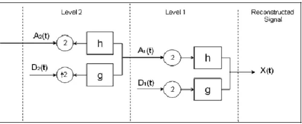
Figure 3.4 DWT reconstruction for 1D signal
Thresholding step is the selection of threshold level for denoising the signal. Since the work of Donoho and Johnstone (Donoho and Johnstone, 1994(a) ; Donoho and Johnstone, 1994(b); Donoho and Johnstone, 1995) there has been a lot of research on the way of defining threshold levels. Their approach suggest, thresholding can be applied soft or hard method, which also called as shrinkage. In 𝑔(𝑛) = 2−1/2〈𝜓(𝑡), 𝜙(2𝑡 − 𝑛)〉 (3.13)
17
hard thresholding wavelet coefficients below a given value is setted to zero. In soft thresholding wavelet coefficients are reduced to the threshold value. A threshold value is the estimation of the signal noise level. It is generally calculated as the standart deviation of detail coefficient (Donoho and Johnstone. 1995). Hard and soft threshold are formulated in equation (3.14) and (3.15) which x is the input signal, y is the signal after threshold and
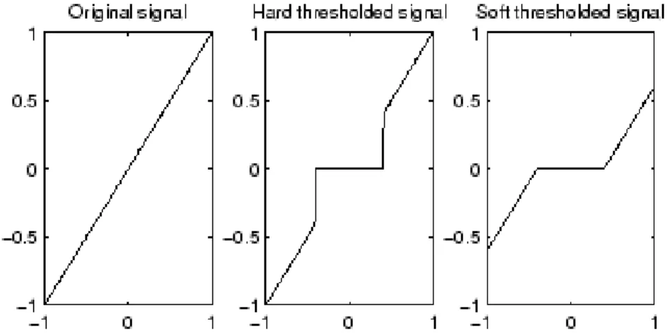
is the threshold value;Figure 3.5 Visualization of hard and soft thresholding
Figure 3.7 shows the visualization of hard and soft threshold method. Hard threshold is a “keep or kill” procedure alternatively soft threshold, shrinks coefficients above the threshold in absolute value. Continuity of soft threshold has beneficial effect that shrinks false structures in the signal. (Joy et al,2013)
Finding the appropriate threshold value is important in de-noising process. There are four main methods for finding this threshold. These are; Universal threshold, Minimax threshold, Rigorous SURE threshold, Heursure method. Universal threshold is known as “sqtwolog” determines a fixed threshold value from soft threshold with Gaussian noise. It is formulated as 2log(n)where the value of ‘n’ indicates the length of the signal and is the standard deviation. This estimation focuses on the data size not the context of the data. It provides a threshold 𝑆𝑜𝑓𝑡 𝑇ℎ𝑟𝑒𝑠ℎ𝑜𝑙𝑑 = {𝑦 = 𝑠𝑖𝑔𝑛(𝑥)(|𝑥| − 𝜆)} (3.15) 𝐻𝑎𝑟𝑑 𝑇ℎ𝑟𝑒𝑠ℎ𝑜𝑙𝑑 = {𝑦 = 𝑥 𝑖𝑓 |𝑥| > 𝜆 𝑜𝑟 𝑦 = 0 𝑖𝑓 |𝑥| < 𝜆} (3.14)
18
value larger than the other algorithms but output is smoother. Another de-noising algorithm is called minimax threshold method. It is derived from minimizing the risk involved in the signal. It is formulated as nwhere n is estimated to reduce the risk in the signal. Rigorous SURE threshold is not a global threshold technique that appropriate threshold is not applied on all of the wavelet coefficients. This method uses a threshold value jat each level j of wavelet coefficients. Lastly, Heursure method is a combination of universal threshold and rigorous SURE threshold. It is useful when the majority of the coefficients are zero. If the set of coefficients is sparse, then the universal threshold is used; otherwise, SURE is applied. (Chourasia and Mittra 2009; Joy et al, 2013)
3.5 Mother wavelet selection
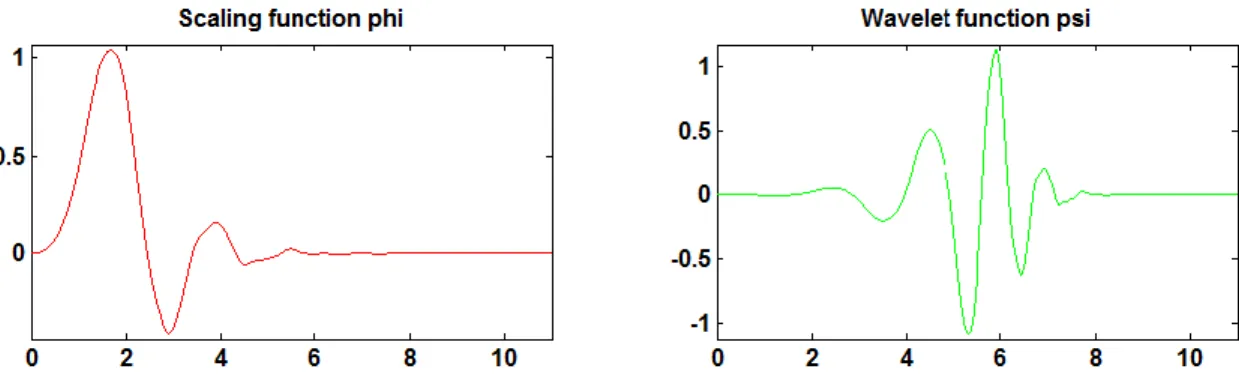
The purpose of wavelets analysis is to analyze non-stationary and transient signals such as power signal. However, when real wavelets are used, the transient characteristics are not resolved appropriately. Using complex wavelets, the magnitude and phase of wavelet coefficients can be separated. Therefore, the energy distribution of the signal can be analyzed by inspecting squared magnitude of the coefficients called as scalogram. In this thesis two different complex mother wavelets which are more suitable for power systems signals have been used for the harmonic analysis. These are “complex Shannon” and “complex Morlet”. Real and imaginary parts of both mother wavelets are in figure 3.2. After the harmonic analysis “Daubechies” wavelet is used for the de-noising algorithm. Figure 3.3 shows the scaling function and wavelet description for the “db6”
Figure 3.6 Description of “cmor0.5-10” and “shan0.5-10
-2 -1 0 1 2 -1 0 1 cmor 0.5-10 Real part (a) -2 -1 0 1 2 -1 0 1 cmor 0.5-10 Imaginary part (b) -2 -1 0 1 2 -1 0 1 shan 0.5-10 Real part (c) -2 -1 0 1 2 -1 0 1 shan 0.5-10 Imaginary part (d)
19
20
4 METHODOLOGY
4.1 Definition of the Plant
Gas turbine based cogeneration systems provides a stable supply of electrical power and can be isolated from the local distribution network. Figure 4 .1 shows that heat is produced either as hot water or as steam for use by the customers. If there is a need for cooling, the heat can be fed into absorption chiller providing a source of cold power. This can be used in air conditioning system. If the system provides electricity, heating and cooling these are called trigeneration plants. In our plant the system only provides electricity, steam and hot water so the unit is a cogeneration system.
Figure 4.1 Gas turbine based cogeneration system
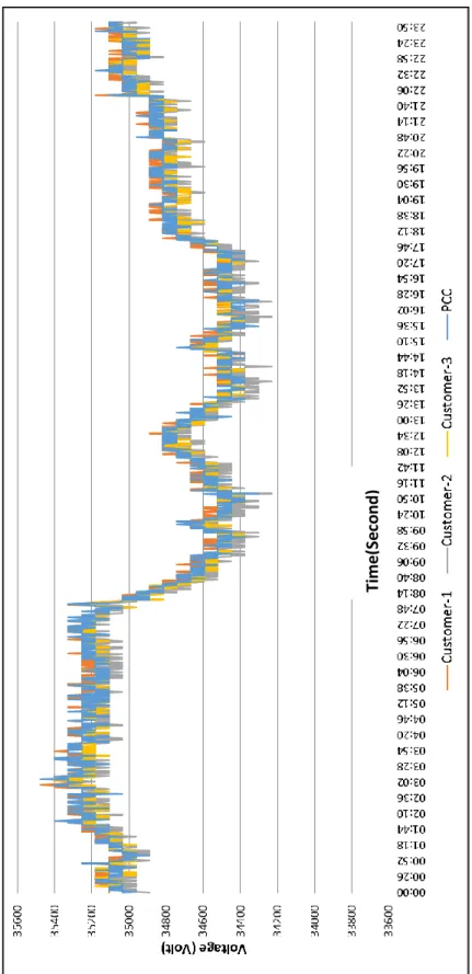
Given in Appedix A, İzmir has 46 distributed generation systems which 27 of them has a heat product. Our system has a 10 MW capacity and connected to the distribution network via 34.5 kV busbar. Cogeneration system includes 2 gas turbines (5 MW each), 3 different customers and a point common coupling (PCC) that connects the system to national grid. Single line diagram of the cogeneration system is given in Appendix B. Current and voltage specifications of these customers are presented in figure 4.2 and figure 4.3. All customers have similar voltage characteristics but due to different power rates current characteristics are different.
21
Figure 4.2 Voltage specifications for all customers
Ti me(S ec o n d )
22
Figure 4.3 Current specifications for all customers
Ti me(S ec o n d )
23
4.2 Harmonic Analysis
Distributed generation design requires many analyses in order to reach optimal working conditions. First of all, power flow analysis must be applied to determine the parameters of the equipment. Short circuit analysis has to be executed in order to determine fault currents, which is necessary for the selecting circuit breakers. For an isolated cogeneration system, transient stability analysis must be done to ensure the stable operation in isochronous mode. (Hsu et al., 2011) Lastly, harmonic analysis is performed for the design of harmonic filters to solve distortion problems and power quality events.
In this thesis, “Fourier Transform” and “Wavelet transform” is used for determining harmonic frequencies in the system. Raw data used in the analysis is recorded in the field by system central computer as “DAT” format. It is recorded in several different operating modes such as island mode, high power mode, low power mode. In this thesis base load operation data is used as a raw data. Recorded signals have 678 data points which form 1 second.
Earlier analysis show that the frequency response of the signal is up to 350 Hz because of the 678 data points. Linear interpolation is used to approximate the value of the signal using two known values at other points. It is applied on the recorded data to enlarge signal to 1355 data points. In this way sampling frequency is made 700 Hz.
“Fast Fourier Transform” is by far the most popular method to analyze signals have multiple frequencies. It is a good way to determine frequency components in a stationary signal whose frequency does not change in time. But real life signals are not stationary and a planner must know in which times these frequency components exist. It has limitations that it only gives the frequency information of the signal; but it does not tell us when in time these frequency components exist. To overcome this problem “wavelet theory” is presented. It gives the time-frequency representation in addition to when frequency component exist in time. Wavelet analysis begins with choosing the right mother wavelet. Mother wavelet selection method is considered in chapter 4.2.1
24 Mother Wavelet Selection
Mother wavelet selection is one of the most compelling things when it comes to applying wavelet transform. Many applications depend on the choice of mother wavelet and the basis of selection is primarily trial and error. Several parameters have to be considered in choosing; such as similarity between the signal and mother wavelet, sampling rate and the duration of the signal and type of information to be extracted from signal. (Ngui et al., 2013)
In this thesis, raw data’s and generated test signal are real valued signal. But it is preferred to select complex valued mother wavelets. Fourier transform of complex valued wavelet is zero for all negative frequencies. By using a complex wavelet we can separate phase and amplitude information of the signal. In this thesis, two different complex valued mother wavelets are used for the harmonic analysis. They are “complex Shannon (shan0.5-10)” and “complex Morlet (cmor0.5-10)”. Both wavelets are selected by proper bandwidth and center frequency parameters. It is also known that they are suitable for continuous wavelet transform. A test signal is generated in order to test the proper mother wavelet. Test signal is formed as;
𝑥(𝑡) = sin(2𝜋50𝑡) + 0.33 sin(2𝜋150𝑡) + 0.20 sin(2𝜋250𝑡) + 0.14 sin(2𝜋350𝑡) First mother wavelet is complex Shannon “shan0.5-10”. Center frequency of selected mother wavelet is 2.9750 Hz. Figure 4.4 indicates all fundamental harmonic and 3 other harmonics in the scalogram; but there are multiple extra frequency components between 0 to 50 Hz. In addition, continuous wavelet coefficients are not computed correctly so that complex Shannon wavelet is not suitable for power system harmonic analysis. Second mother wavelet is complex Morlet “cmor0.5-10”. Center frequency is calculated as 5.9375 Hz. This wavelet has a complex sinusoid with a Gaussian envelope. Complex part shows the real and imaginary parts. Scaled and dilated cmor wavelet is applied on the test signal in figure 4.5. Results show that all frequency components and amplitudes are calculated correctly. Complex Morlet wavelet is the optimal mother wavelet for this application.
25
Figure 4.4 Complex Shannon wavelet analysis
Figure 4.5 Complex Gaussian wavelet analysis
Time(s) (a) F re q u e n c y (H z)
Mother wavelet: shan0.5-10
0 0.1 0.2 0.3 0.4 0.5 0.6 0.7 0.8 0.9 50 100 150 200 250 300 350 400 450 500 Time(s) (c) F re q u e n c y (H z)
Mother wavelet: cmor0.5-10
0 0.1 0.2 0.3 0.4 0.5 0.6 0.7 0.8 0.9 50 100 150 200 250 300 350 400 450 500
26 Harmonic Analysis on Raw data
In a cogeneration unit, on-site generator will track the grid voltage in acceptable limits. If this situation fails, the link between grid and on-site generator will be broken. This can be caused by power quality events or huge load variations. Any disturbance will affect entire system. Voltage dips, sags, swells and interruptions effect many microprocessor based equipment. In addition to these power quality events, harmonic components can also appear in the system. Electrical motors, UPS devices, adjustable speed drives etc. are harmonic sources. These harmonic sources can cause over heating by excessive currents, overloading capacitor banks which is used for power factor correction, power line disturbance problems with electronic and computer control systems and telephone interference. In this thesis, harmonic analysis is done by 2 different algorithms. Fast Fourier algorithm gives a frequency response of the signal with respect to their amplitudes. Wavelet algorithm gives the time-frequency spectrum of the signal. All raw data’s used in this study are logged by using data logger in center computer. Diagram of the plant is demonstrated in figure 4.6
Figure 4.6 Diagram of the cogeneration plant
PCC
Customer-0
Customer-1
Customer-2
Customer-3
Gas Turbine-1
Gas Turbine-2
27
Customer-0 indicates the facility that consist the cogeneration unit. Customer 1 is a beverage facility that has an installed power of 9 MVA. It has 12 compressor units which located in cooling and compressed air. They do not need to perform any harmonic measurement because they don’t encounter any harmonic related incident. Customer-0 center computer logged three phase voltage and current raw data’s from the distribution network. Figure 4.7(a) indicates three phase current drawn from the customer-1. Phase A is chosen for the harmonic analysis which can be seen on figure 4.7 (b)
Figure 4.7 Customer-1 current
In figure 4.8 (a), Fourier spectrum of customer-1 shows there is a 5th and 7th harmonic distortion in the system. There are multiple inter harmonic components located in 326.6 Hz and 426.7 Hz. Due to limitations of Fourier spectrum it is only seen where the frequency components located. Later; chosen mother wavelet “cmor 0.5-10” is scaled and applied to the system. Scalogram in figure 4.8 proves that there is a 5th and 7th harmonic distortion in the system. Wavelet coefficients are gathered on specific harmonic frequencies. Darkest color on the scalogram shows the highest amplitude of the frequency. It is also seen there is an instantaneous change in amplitude during 0.15 seconds.
0 0.1 0.2 0.3 0.4 0.5 0.6 0.7 0.8 0.9 -50 0 50 Time(s) (a) C u rr e n t( A ) 0.4 0.45 0.5 0.55 0.6 -50 0 50 Time(s) (b) C u rr e n t( A )
28
Figure 4.8 Fourier spectrum and Scalogram of customer-1 (a) Fourier Spectrum (b) Scalogram
Customer-2 is a factory in food industry which has a total capacity of 8 MVA. It supply electric and steam from the cogeneration unit. It has 9 electric motors over 100 kW which has a speed between 1400-2800 rpm. These motors are used in cooling, air conditioning and in homogenizer units. Customer-2 made a harmonic measurement back in 2010. Current and voltage harmonic values come up under the standard limits. But there are harmonic filters in the low distribution side. Figure 4.9 shows current waveform of customer-2. Customer-2 has drawn approximately 54 A. Current is nearly sine waveform. Harmonic components are too small so that can be neglected.
Customer 3 is a factory in animal feed sector. It draws less current than the other customers. Figure 4.11 (a) shows the three phase current of the customer-3. Phase A is chosen for the harmonic analysis which can be seen on figure 4.11 (b). Harmonic analysis on figure 4.12 shows there are multiple harmonic components in the spectrum. Inter-harmonics can be seen in the scalogram. Deeper analysis must be done in order to find the source of the harmonics.
0 100 200 300 400 500 600 -100 -50 0 50 Frequency(Hz) (a) A m p li tu d e (d B ) Time(s) (b) F re q u e n c y (H z) 0 0.1 0.2 0.3 0.4 0.5 0.6 0.7 0.8 0.9 200 400 600
29
Figure 4.9 Customer-2 current
Figure 4.10 Fourier spectrum and Scalogram of customer-2 (a) Fourier Spectrum (b) Scalogram
0 0.1 0.2 0.3 0.4 0.5 0.6 0.7 0.8 0.9 -50 0 50 Time(s) (a) C u rr e n t( A ) 0.4 0.45 0.5 0.55 0.6 -50 0 50 Time(s) (b) C u rr e n t( A ) 0 100 200 300 400 500 600 -100 -50 0 50 Frequency(Hz) (a) A m p li tu d e (d B ) Time(s) (b) F re q u e n c y (H z) 0 0.1 0.2 0.3 0.4 0.5 0.6 0.7 0.8 0.9 200 400 600
30
Figure 4.11 Customer-3 current (baseload)
Figure 4.12 Fourier spectrum and Scalogram of customer-2 (a) Fourier Spectrum (b) Scalogram
0 0.1 0.2 0.3 0.4 0.5 0.6 0.7 0.8 0.9 -10 0 10 Time(s) (a) C u rr e n t( A ) 0.4 0.45 0.5 0.55 0.6 -10 0 10 Time(s) (b) C u rr e n t( A ) 0 100 200 300 400 500 600 -150 -100 -50 0 Frequency(Hz) (a) A m p li tu d e (d B ) Time(s) (b) F re q u e n c y (H z) 0 0.1 0.2 0.3 0.4 0.5 0.6 0.7 0.8 0.9 200 400 600
31
4.3 Filtering and de-noising
A low-pass filter allows the signals below cutoff frequency and attenuates signals above the cutoff frequency. Filters are designed by defining their passband and stopband. By removing higher frequencies filter creates a smoothing effect. When a filter applied to a signal it produces slow changes in the output values. In this case it is easier to see any change in the signal-to-noise ratio with minimal signal degradation. Low-pass filters like moving average filter or Savitzky-Golay filter are often used to remove noise, data averaging and discover important patterns. (Mathworks, 2015)
MATLAB signal processing toolbox has a filter visualization tool named as “fdatool”. Figure 4.13 shows the basic concepts of this analysis tool. In this thesis a low pass filter is designed to mitigate harmonics. Filter coefficients exported and saved in MATLAB workspace. After that it is performed a convolution between raw data and filter coefficients to get the filtered output.
32
Figure 4.14 Low-pass filter specification
Designed low pass filter has a finite impulse response (FIR). FIR filters are designed by finding filter coefficients and filter order that meat a certain specification. Fdatool gives the knowledge of filters impulse response. This allows a process called convolution in time domain. Visualization of filter specifications is shown in figure 4.14.
Table 4.1 Lowpass FIR filter specifications
Passband frequency Passband ripple Sampling frequency Filter order Stopband frequency Stopband Ripple 75 Hz 0.5 dB 1356.9 Hz 12 190 Hz 20 dB
After all the parameters are entered in fdatool, filter coefficients are computed. Designed filter is a direct-form FIR filter which is order of 12. Filter coefficients are exported in MATLAB workspace in order to load in convolution process. Magnitude response is shown in figure 4.15. As it can be seen in the figure, after the convolution it is desired to reduce the harmonics 20 dB.
33
Figure 4.15 Magnitude response of low-pass filter
The main study of this thesis is based on harmonic filtering by using wavelet de-noising algorithm. Main challenge of using de-noising algorithm is to define the proper threshold value. Finding the most convenient threshold value is extended to Donoho and Johnstone work.(Donoho and Johnstone,1994(b)). Joy et al., 2013 states “Motivation to thresholding is based on the assumptions that the decorrelating property of a wavelet transform creates a sparse signal: most untouched coefficients are zero or close to zero. There must be a balance in choosing appropriate threshold value. A very large threshold cuts too many coefficients, resulting in an over smoothing. Conversely, a too small threshold value allows many coefficients to be included in reconstruction, giving a wiggly, under smoothed estimate.” (Joy et al. 2013). Generally; threshold choosing methods are divided into global thresholding and level-dependent thresholding. Global method is applied to all wavelet coefficients but as the name implies level-dependent method is changed for each wavelet level.
In this thesis, it is used two different functions to calculate threshold value and application of de-noising. ‘ddencmp’ returned default values for de-noising or compression, using either a wavelet or wavelet packet. Result of this function gives a fixed threshold value by using “Universal threshold” formula and the choice of soft or hard threshold. On the other hand ‘wdencmp’ function performs a de-noising or
0 100 200 300 400 500 600 -60 -50 -40 -30 -20 -10 0 Frequency (Hz) M a g n it u d e ( d B )
34
compression of a signal using wavelet. First of all signal is decomposed its detail wavelet coefficients. After that, soft thresholding is applied. Lastly, signal is reconstructed with using original approximation coefficients and modified detail coefficients.
In the following; harmonics which have found in earlier chapters are filtered and de-noised. A level 2 wavelet Daubechies ‘db 6’ is chosen for the comparison with designed FIR filter. Characteristic of a FIR filter creates a group delay. Group delay of a linear phase FIR filter is constant for all frequencies because impulse response is symmetrical. Linear phase can be defined as that all frequencies input signal experience the same delay. It can be calculated as (N-1)/2 samples for N is the filter length. Choice of level of decomposition is also important in wavelet analysis. In the low frequency region delay can cause small phase shift; but in a noisy region peak values can change. On the high frequency region, phase shift can cause instability.
Customer-1 and customer-3 are used as a raw data for the performance analysis of filter and de-noise algorithm. Threshold value is calculated for each customer. Filter response for customer-1 is shown in figure 4.16 (a). Harmonics are reduced 20 dB in figure .16 (b). There is a group delay which caused by the filter characteristic. De-noise algorithm is applied on the customer-1 data in figure 4.17. Calculated threshold for customer-1 is 27.9950. Root mean square error between original and de-noised signal is 0.1606. Filter response for customer-3 is shown in figure 4.18. Calculated threshold for customer-3 is 9.4912. De-noising algorithm response is shown in figure 4.19. Root mean square error between original and de-noised signal is 0.0350. For both of the customers there is no phase shift and harmonics are reduced very well.
As it can be seen in the figures, de-noising algorithm response is better than the FIR filter scheme. In real time applications data alignment is a serious problem. For basic current de-noising, simple FIR filters are better to use because it is implemented simple and low-cost hardware or with some additions to a software. But in the cases where there is need to be extracted useful information like adjustable speed drives, motor stator etc. wavelets should be preferred.
35
Figure 4.16 Customer-1 filtered harmonics
Figure 4.17 Customer-1 de-noised harmonics
0.48 0.5 0.52 0.54 0.56 0.58 0.6 0.62 -50 0 50 Time(s) (a) C u rr e n t( A ) 0 50 100 150 200 250 300 350 400 450 500 -300 -200 -100 0 100 Frequency(Hz) (b) A m p li tu d e ( d B ) 0.48 0.5 0.52 0.54 0.56 0.58 0.6 0.62 -50 0 50 Time(s) (a) C u rr e n t( A ) 0 50 100 150 200 250 300 350 400 450 500 -200 -100 0 100 Frequency(Hz) (b) A m p li tu d e ( d B )
36
Figure 4.18 Customer-3 filtered harmonics
Figure 4.19 Customer-3 de-noised harmonics
0.48 0.5 0.52 0.54 0.56 0.58 0.6 0.62 -10 0 10 Time(s) (a) C u rr e n t( A ) 0 50 100 150 200 250 300 350 400 450 500 -300 -200 -100 0 100 Frequency(Hz) (b) A m p li tu d e ( d B ) 0.48 0.5 0.52 0.54 0.56 0.58 0.6 0.62 -10 0 10 Time(s) (a) C u rr e n t( A ) 0 50 100 150 200 250 300 350 400 450 500 -200 -100 0 100 Frequency(Hz) (b) A m p li tu d e ( d B )