Compressed sensing techniques for accelerated magnetic resonance imaging

COMPRESSED SENSING TECHNIQUES

FOR ACCELERATED MAGNETIC

RESONANCE IMAGING

a thesis submitted to

the graduate school of engineering and science

of bilkent university

in partial fulfillment of the requirements for

the degree of

master of science

in

electrical and electronics engineering

By

Efe Ilıcak

July 2017

Compressed sensing techniques for accelerated magnetic resonance imaging

By Efe Ilıcak July 2017

We certify that we have read this thesis and that in our opinion it is fully adequate, in scope and in quality, as a thesis for the degree of Master of Science.

Tolga C¸ ukur(Advisor)

Emine ¨Ulk¨u Sarıta¸s C¸ ukur

Beh¸cet Murat Ey¨ubo˘glu

Approved for the Graduate School of Engineering and Science:

Ezhan Kara¸san

ABSTRACT

COMPRESSED SENSING TECHNIQUES FOR

ACCELERATED MAGNETIC RESONANCE IMAGING

Efe Ilıcak

M.S. in Electrical and Electronics Engineering Advisor: Tolga C¸ ukur

July 2017

Magnetic resonance imaging has seen a growing interest in the recent years due to its non-invasive and non-ionizing nature. However, imaging speed remains a ma-jor concern. Recently, compressed sensing theory has opened new doors for accel-erated imaging applications. This dissertation studies compressed sensing based reconstruction strategies for accelerated magnetic resonance imaging, specifically for angiography and multiple-acquisition methods. For magnetic resonance an-giography, we propose a novel approach that improves scan time efficiency while suppressing background signals. In this study, we attain high-contrast angiograms from undersampled data by utilizing a two-stage reconstruction strategy. Simula-tions and in vivo experiments demonstrate that the developed strategy is able to relax trade-offs between image contrast and scan efficiency without compromising vessel depiction. For multiple-acquisition balanced steady state free precession imaging, we develop a framework that jointly reconstructs undersampled phase-cycled images. This approach is able to improve banding artifact suppression while maintaining scan efficiency. Results show that the proposed method is able to attain high-quality reconstructions even at high acceleration factors.

Overall, the findings presented in this thesis indicate that compressed sensing reconstructions represent a promising future for rapid magnetic resonance imag-ing. Consequently, compressed sensing reconstruction techniques hold a great potential to change the time-consuming clinical imaging practices.

¨

OZET

HIZLANDIRILMIS

¸ MANYET˙IK REZONANS

G ¨

OR ¨

UNT ¨

ULEME ˙IC

¸ ˙IN SIKIS

¸TIRILMIS

¸ ALGILAMA

TEKN˙IKLER˙I

Efe Ilıcak

Elektrik ve Elektronik M¨uhendisli˘gi, Y¨uksek Lisans Tez Danı¸smanı: Tolga C¸ ukur

Temmuz 2017

Manyetik rezonans g¨or¨unt¨uleme, invazif ve iyonla¸stırıcı olmamasından dolayı son yıllarda artan bir ilgi g¨ormektedir. Ancak g¨or¨unt¨uleme hızı, temel bir problem te¸skil etmektedir. Yakın zamanda sıkı¸stırılmı¸s algılama kuramı, hızlandırılmı¸s g¨or¨unt¨uleme uygulamaları i¸cin yeni fırsatlar olu¸sturmu¸stur. Bu tez, ¨ozellikle an-jiyografi ve ¸coklu ¸cekim y¨ontemlerinde kullanılmak ¨uzere geli¸stirilmi¸s, sıkı¸stırılmı¸s algılama kuramına dayalı geri¸catım tekniklerini incelemektedir. Manyetik rezo-nans anjiyografi i¸cin, g¨or¨unt¨u s¨uresi verimlili˘gini artırırken arkaplan sinyallerini baskılayan yeni bir y¨ontem ¨onerilmi¸stir. Bu ¸calı¸smada y¨uksek kontrastlı anjiyo-gramlar, eksik ¨orneklendirilmi¸s veriden iki a¸samalı bir geri¸catım tekni˘gi ile elde edilmektedir. Geli¸stirilen y¨ontemin g¨or¨unt¨u kontrastı ile g¨or¨unt¨uleme verimlili˘gi arasındaki dengeyi, damar g¨orselli˘gini bozmadan gev¸setebildi˘gi, simusayon ve in vivo deneyler ile g¨osterilmi¸stir. C¸ oklu ¸cekim dengeli kararlı-durum serbest devinim g¨or¨unt¨uleme teknikleri i¸cin ise, eksik ¨orneklendirilmi¸s faz d¨ong¨ul¨u g¨or¨unt¨uleri birlikte i¸sleyen bir geri¸catım tekni˘gi geli¸stirilmi¸stir. Bu y¨ontem g¨or¨unt¨uleme verimlili˘gini korurken, b¨uk¨ulme artifaktlarının baskılanmasını iy-ile¸stirebilmektedir. Elde edilen sonu¸clar, bu y¨ontemin y¨uksek hızlandırma de˘gerlerinde bile y¨uksek kaliteli geri¸catımlar elde edebildi˘gini g¨ostermektedir.

Sonu¸c olarak bu tezdeki bulgular, sıkı¸stırılmı¸s algılamaya ba˘glı geri¸catım y¨ontemlerinin, hızlı manyetik rezonans g¨or¨unt¨uleme i¸cin umut vadeden bir geli¸sme oldu˘gunu g¨ostermektedir. Buna ba˘glı olarak sıkı¸stırılmı¸s algılama geri¸catma tekniklerinin, zaman alıcı klinik g¨or¨unt¨uleme uygulamalarını de˘gi¸stirmek i¸cin b¨uy¨uk bir fırsat sundu˘gunu g¨or¨ulmektedir.

v

Acknowledgement

First of all, I would like to express my sincere gratitude to Prof. Tolga C¸ ukur, who has supported me with his endless guidance. This thesis would not been possible without his wisdom and his confidence in me. He has given me the tools as well as the freedom to pursue my research interests.

I would like to extend my thanks to Prof. Sarıta¸s. Her precious insights and her unparalleled teaching skill have taught me what I know about MRI and many imaging modalities.

I would also like to thank Prof. Atalar for founding UMRAM and providing this amazing environment. With his vision, we are able embark on academic endeavors and be at the forefront of scientific discovery.

During my time at UMRAM and ICON Lab, I was lucky enough to know and work with many great people. In particular, I am grateful to ¨Umit Kele¸s,

¨

Ozg¨ur Yılmaz, Toygan Kılı¸c, Salman Dar for helping me throughout this journey and Erdem Bıyık for being the perfect intern. I would also like to thank Aydan Ercing¨oz for creating order from chaos and keeping UMRAM functioning; Umut G¨undo˘gdu and Mustafa Can Delikanlı for teaching me how to use MRI scanner and helping me with my never-ending questions.

I also owe special thanks to my brother from another mother, Uras Demir; and my dear friends, Canberk Pay, Goks¨u Yama¸c, Emir Artık, and Sezer Yılmazer for all the help and motivation they provided me to write this thesis.

Last but not the least, I would like to thank my family, my mother Meltem, my father Sinan and my brother Ege, for their endless love and unconditional support. Words cannot describe how grateful I am. Without them, none of this would be possible.

Contents

1 Introduction 1

1.1 Outline of the thesis . . . 4

2 Targeted vessel reconstruction for vessel preservation in non-contrast-enhanced angiography 6 2.1 Introduction . . . 8 2.2 Methods . . . 9 2.2.1 Pulse Sequence . . . 11 2.2.2 Sampling Patterns . . . 11 2.2.3 Vasculature Mapping . . . 12

2.2.4 Targeted Compressed-Sensing Reconstructions . . . 14

2.2.5 Simulations . . . 17

2.2.6 Experiments . . . 21

CONTENTS viii

2.4 Discussion . . . 33

3 Profile encoding reconstruction for multiple-acquisition balanced steady-state free precession imaging 36 3.1 Introduction . . . 38

3.2 Methods . . . 39

3.2.1 Undersampling Patterns for Multiple-Acquisition bSSFP Data . . . 42 3.2.2 Profile-Encoding Reconstruction . . . 42 3.2.3 Alternative Reconstructions . . . 47 3.2.4 Simulations . . . 48 3.2.5 In Vivo Experiments . . . 50 3.3 Results . . . 51 3.3.1 Simulation Analyses . . . 51 3.3.2 In Vivo Analyses . . . 60 3.4 Discussion . . . 64 4 Conclusion 67 4.1 Future Work . . . 68

4.2 Contributions to the Literature . . . 68

CONTENTS ix

4.2.2 Conference Papers . . . 69

List of Figures

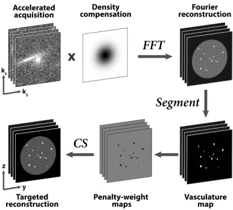
2.1 Proposed reconstruction strategy. Angiograms with variable-density undersampling in k-space are variable-density-compensated and transformed to obtain Fourier reconstructions (ZF). A segmenta-tion algorithm is then employed to trace vessel trees across the volume. In conventional CS, penalty terms are weighted uniformly across images. Here penalty weights are selected based on seg-mented vasculature maps: smaller weights at vessel locations en-abling targeted reconstructions. Note that data are not density compensated during CS, but only to obtain ZF used for segmen-tation. . . 10

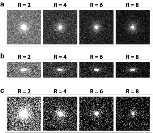
2.2 Variable-density random sampling masks used at each acceleration factor R=2-8. (a) Sampling masks (384×384) for phantom data. (b) Sampling masks (240×110) for hand data. (c) Sampling masks (128×128) for lower leg and foot data. . . 12

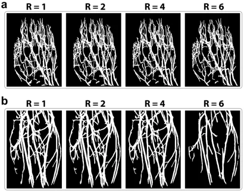
2.3 Vasculature maps were segmented from undersampled angiograms at acceleration factors R = 1-6. Vessel volumes for hand an-giograms (a) and lower leg anan-giograms (b) are visualized with maximum-intensity projections (MIPs). Segmentation results at R = 1 (fully-sampled), 2 and 4 are visually similar to each other. For higher R, losses in vessel volume are apparent particularly small vessels. The percentage volume loss in each map is listed with respect to the ideal map at R = 1. . . 13

LIST OF FIGURES xi

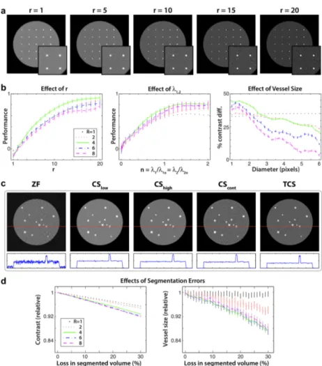
2.4 (a) A phantom with 25 blood vessels of sizes 0.33 to 2 mm en-closed by muscle. Targeted CS (TCS) reconstructions were cal-culated using r ∈ [1 20], λ1,2 = λ1o,2o, and R = 1-8. Results are

shown for R = 4, with magnified lower-right portions of images. Higher r enhance blood/muscle contrast, but image distortions be-come prominent for r ≥ 15. (b) TCS performance was taken as the ratio of contrast improvement to dispersion level (mean±sem across vessels). For all R, r = 10 and λ1,2 = λ1o,2o yield close

to optimal reconstruction performance (left and middle panels). TCS using λ1,2 = λ1o,2o and r = 10 was repeated for 20 random

instances additive noise. Contrast improvement is plotted for each vessel diameter (right panel; mean±sem across 20 images). The improvement is greater for smaller vessels. (c) A separate phantom with 13 blood vessels of sizes 1.25 to 3.75 mm. Fourier reconstruc-tions (ZF), conventional CS, and TCS were calculated for R = 4. The panel below each image shows a sample line profile (across the red line). TCS improves blood/muscle contrast without significant image distortions. (d) TCS reconstructions were obtained while losses in segmented vessel maps were simulated by random erosions of the ideal map. Contrast and vessel sizes were measured relative to a TCS reconstruction based on the ideal map (mean±sem across 20 instances of erosion). . . 20

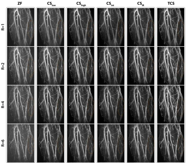
2.5 Lower-leg angiograms reconstructed using conventional CS with uniformly-weighted penalty terms (CSlow, CShigh), CS with

spatially-weighted penalty terms based on intensity of ZF recon-structions (CSint), iteratively-reweighted CS (CSIR), and TCS.

Representative axial sections are shown for R = 4. CShigh,

CSint and CSIR suffer from signal losses, particularly in relatively

small or low intensity vessels. In contrast, TCS improved back-ground suppression while preserving detailed depiction of vascula-ture (marked with ellipses and arrows). . . 25

LIST OF FIGURES xii

2.6 MIPs of hand angiograms reconstructed with ZF, CSIR and TCS,

for R = 1-6. CSIR suffers increasingly from loss of small vessels

for higher R. Furthermore, bright synovial fluid causes suboptimal vessel contrast in ZF and CSIR. In contrast, TCS alleviates vessel

loss while improving suppression of background signals (marked with arrows). . . 26

2.7 MIPs of lower leg angiograms reconstructed with ZF, CSIR and

TCS, for R = 1-6. There is visible loss of low-intensity and small vessels in CSIR. TCS achieves improved blood/muscle contrast

with no visible vessel loss up to R = 4 (marked with ellipses). Due to reduction of segmented volumes for R = 6 (Fig. 2.3), some small vessels are depicted suboptimally. . . 27

3.1 In the profile-encoding framework, each phase-cycled bSSFP im-age (Sn) is modeled as the multiplication of an ideal image free of

banding artifacts (So) with a respective bSSFP sensitivity profile

(Cn). The value of the bSSFP profile at each location is a function

of total phase accrual over a single TR due to main field inho-mogeneity and RF phase-cycling increment (∆φ). Locations of near-zero phase shift (modulo 2π) lead to significantly diminished sensitivity and thereby banding artifacts in bSSFP images. . . . 41

LIST OF FIGURES xiii

3.2 Flowchart of the profile-encoding bSSFP (PE-SSFP) reconstruc-tion that recovers missing data in undersampled phase-cycled ac-quisitions. PE-SSFP employs an alternating projection-onto-sets scheme with four projection operators: calibration, joint-sparsity, TV, and data-consistency projections. In the calibration projec-tion, an interpolation kernel estimated from calibration data is used to synthesize missing samples linearly from acquired data across phase-cycles. In the joint-sparsity projection, wavelet coeffi-cients of phase-cycled bSSFP images are thresholded with a Huber function. In the TV projection, bSSFP images are denoised with a fast iterative-clipping algorithm. In the data-consistency pro-jection, reconstructed data in sampled locations are replaced with their acquired values. These projections are successively repeated, and the individual phase-cycled images are finally combined with the p-norm method. . . 44

3.3 Phase-cycled bSSFP images of a numerical phantom were simu-lated for N=2-8, α = 45o_{, TR/TE=5.0/2.5 ms, a field map of 0±62}

Hz (mean±std). Phantom images were undersampled by a factor of N via variable-density random sampling, disjointly across phase cycles. Zero-filled Fourier (ZF, top row), individual compressed sensing (iCS, middle row), and PE-SSFP (bottom row) reconstruc-tions are shown. White boxes display a zoomed-in portion of the images. ZF reconstructions suffer from elevated aliasing/noise in-terference at high N due to the heavier undersampling factors used. While iCS reconstructions employ regularization terms that limit this interference, the heavy undersampling factors at high N cause visible loss of spatial resolution. In contrast, PE-SSFP successfully alleviates noise and aliasing interference while maintaining detailed depiction of tissue boundaries. . . 52

LIST OF FIGURES xiv

3.4 Representative bSSFP images of the numerical phantom for N=4 were reconstructed using ZF and PE-SSFP. Images from three vari-ants of PE-SSFP are shown (top row). PEcalibonly uses calibration

and data-consistency projections, PEhuber uses calibration,

joint-sparsity and data-consistency projections, and PE-SSFP addition-ally uses TV projections. Reconstructions were compared against a combination of fully-sampled images (for N=8). Squared-error maps are shown in logarithmic scale (bottom row; see colorbar). Each additional projection in PE-SSFP yields visibly reduced re-construction error in bSSFP images. . . 54

3.5 The noise-amplification maps for ZF, iCS and PE-SSFP meth-ods are displayed for N=2-8. Although the heavier undersampling at high N increases noise amplification in ZF reconstructions, re-constructions with penalty terms iCS and PE-SSFP maintain rel-atively low noise amplification even at high N. The lower noise amplification with iCS likely reflects a bias from excessive loss of high-spatial-frequency information. In PE-SSFP, relatively higher amplification is observed near tissue boundaries that are more sus-ceptible to resolution loss due to variable-density undersampling. 55

3.6 Phase-cycled bSSFP reconstructions of the numerical phantom (top row), and the squared-error maps with respect to the fully-sampled combination image (bottom row) are displayed for N=8. ZF has broadly distributed errors across the field-of-view due to aliasing and noise interference. iCS reconstructions reduce this interference via TV regularization at the expense of elevated er-rors near tissue boundaries, due to significant loss of high-spatial-frequency information. While ESPIRiT reconstructions alleviate this loss via joint-sparsity penalties, the respective images still show broadly distributed errors. In contrast, PE-SSFP using both joint-sparsity and TV regularization further dampens the recon-struction errors in phase-cycled bSSFP images. . . 57

LIST OF FIGURES xv

3.7 In vivo bSSFP acquisitions of the brain (a) and the knee (b) were reconstructed using PE-SSFP. Squared-error maps are shown in logarithmic scale (see colorbar). The error maps clearly suggest that banding artifact suppression improves for higher N, while PE-SSFP maintains detailed depiction of high-spatial-frequency information. . . 61

3.8 In vivo phase-cycled bSSFP reconstructions of the brain (a) and the knee (b) are displayed for N=8. ZF and ESPIRiT reconstruc-tions suffer from broadly distributed reconstruction error across the images. Meanwhile, iCS reconstructions show substantial loss of high-spatial-frequency information and coherent low-frequency interference. In contrast, PE-SSFP effectively reduces errors due to aliasing and noise interference, while maintaining detailed tissue depiction. . . 62

List of Tables

2.1 Reconstruction Parameters . . . 16

2.2 Contrast and Resolution: Simulated data . . . 24

2.3 Contrast: Representative Single-Subject Hand Data . . . 28

2.4 Contrast: Representative Single-Subject Lower Leg Data . . . 29

2.5 Contrast: Population Lower Leg Data . . . 30

2.6 Contrast: Population Foot Data . . . 31

2.7 Radiological Assessment of Image Quality . . . 32

3.1 Regularization Parameters . . . 46

3.2 Image Assessments for the Brain Phantom . . . 59

Chapter 1

Introduction

Magnetic resonance imaging (MRI) is a noninvasive imaging modality that does not require the use of ionizing radiation. Thanks to its safety and unparalleled soft tissue contrast properties, it has gained widespread usage in the clinical set-tings [1, 2]. However, the incorporation of MRI techniques into clinical practice has been hindered due to its relatively long examination times compared to other imaging modalities such as computed tomography or ultrasound imaging [2, 3]; where this limitation arises from both physical and physiological constraints [4]. Over the last decades, many successful approaches have been proposed to improve the scan efficiency, such as the development of fast switching magnetic field gra-dients; implementation of rapid imaging sequences(e.g., gradient-echo, fast-spin echo, or steady-state free precession sequences); development of multiple coil re-ceiver arrays and parallel imaging techniques, and more recently by using sparsity based compressed sensing applications [5, 3, 6, 4].

Originally emerged from information theory, compressed sensing aims to recon-struct signals from relatively small number of samples compared to traditionally required [7]. This is partly possible due to the compressibility of the underlying signal in a known transform domain. Successful application of compressed sens-ing can be summarized in three requirements: (a) The sampled signal should be sparse or compressible in a known transform domain (e.g., wavelet domain), (b)

the sampling should create incoherent aliasing artifacts in the compression trans-form domain, (c) a nonlinear reconstruction algorithm should be used to enforce sparsity and data consistency. When these three requirements are met, signals can be recovered from significantly lower number of samples [4, 8, 9]. For MRI, these conditions can be matched since MR images are known to be compressible, incoherence can be achieved through random undersampling in k-space, and fi-nally there are efficient algorithms for nonlinear reconstructions [7]. With MRI being a natural fit and its potential to reduce scan time constraints, compressed sensing has sparked a great interest in the MRI community with applications including, but not limited to, anatomical imaging and angiography [4, 8].

Magnetic imaging methods that provide the visualization of blood vessels are referred as magnetic resonance angiography (MRA) methods. These methods can be categorized into two main groups, contrast-enhanced (CE-MRA) and non-contrast-enhanced (NCE-MRA), with the prior utilizing intravenous injection of contrast agents to visualize blood vessels and the later utilizing the intrinsic properties of blood tissue. In the case of non-contrast-enhanced angiography (NCE-MRA), time-of-flight and phase contrast methods rely on the motion of the blood and steady-state method relies on the magnetic properties of blood to generate contrast between vasculature and tissue [10]. Contrast-enhanced MRA methods have gained popularity due to their ease of use, and their ability to quickly produce high-quality diagnostic images of large vascular territories. Cur-rently, Gadolinium-based contrast agents (GBCA) are the most commonly used contrast materials. Since their approval in the 1980s, they have been an im-portant tool for lesion detection and characterization [11]. Similar to computed tomography angiography, CE-MRA provides reliable enhancement of the arte-rial lumen during the artearte-rial phase of the Gadolinium bolus injection, and can rival digital subtraction angiography in image quality and diagnostic accuracy [12]. However, the bolus timing requirements limit the temporal resolution, spa-tial resolution, signal-to-noise ratio; the addition of contrast agent increases the already expensive scan cost; and recent studies identified a connection between the GBCAs and a fatal condition called nephrogenic systemic fibrosis in patients with advanced renal diseases [13, 14, 15, 11]. Besides the financial and safety

benefits, the NCE-MRA examinations can be repeated in case of patient motion or technical errors, and can serve as backup examinations before the injection of contrast agents [15].

As a consequence, the advantages has spurred a renewed interest in the NCE-MRA methods [14]. This resurgence of interest ranges from imaging the renal arteries in the abdomen to cerebral arteries, from thoracic aorta to distal vessels [13, 16, 17, 18, 19]. The NCE-MRA methods can be categorized into two classes: flow-dependent and flow-independent. The early non-contrast techniques such as time-of-flight (TOF) and phase contrast (PC) methods generate the contrast by using the fact that blood is flowing inside stationary tissue. However, these methods suffer from reduced contrast in slow or retrograde flow regions, as seen in the cases with stenosis [19]. In contrast, the flow-independent techniques such as balanced steady-state free precession (bSSFP) depend on the magnetic properties of blood tissue and can generate blood-background contrast even in the cases of slow flow [14, 8]. While these methods have proven their usefulness in offering sensitive assessments of vessel morphology, high spatial resolution is needed for diagnostic quality [20]. Furthermore, given the fact that spatial resolution is directly related to acquisition time, the image quality can be limited by the scan time constraints. Therefore, acceleration strategies that improve scan efficiency can greatly increase the clinical potential of NCE-MRA. As a result, many recent studies have proposed various techniques to accelerate acquisitions, including view-ordering [21], parallel imaging [22, 23, 20], and more recently compressed sensing methods [8, 20, 24, 25].

Another important application of compressed sensing can be found in the usage of bSSFP sequence for anatomical imaging. In recent year, bSSFP sequence has gained popularity as it can provide high signal to noise ratio in short repetition times; and found wide use in numerous MRI applications, such as musculoskele-tal imaging, interventional imaging [26, 27, 28, 29, 30, 31]. However, the bSSFP signal depends on the local resonant frequency and magnetization profile, which yields increased sensitivity to magnetic field inhomogeneities. Therefore, bSSFP sequence suffers from irrecoverable signal losses, called banding artifacts, in re-gions with large off-resonant frequencies [29, 31, 32]. A common approach to

mitigate the banding artifacts is to use multiple-acquisition bSSFP technique [33, 32]. In this method, spatially non-overlapping banding artifacts are cre-ated by acquiring the images by either changing the center frequency directly or by altering the radio frequency pulse between repetition times. Afterwards, the phase-cycled images can be combined to obtain artifact free image. Unfortu-nately, the speed advantage of this sequence is diminished due to the prolonged acquisition time with additional acquisitions. Thus, acceleration strategies that improve the scan efficiency are of great interest.

1.1

Outline of the thesis

Chapter 2 focuses on a novel approach that improves scan efficiency while sup-pressing background signals for accelerated MRA acquisitions. In this work, we attain high-contrast angiograms from undersampled data by utilizing a two-stage reconstruction strategy. In the first step, we generate 3D vessel maps using a tractographic segmentation on Fourier reconstructions of undersampled data. In the second step, targeted reconstructions are performed based on these maps with spatially adaptive `1-norm and total-variation penalties to dampen

back-ground signals while preserving the depiction of vasculature. Simulations and in vivo experiments demonstrates that the developed strategy is able to relax trade-offs between image contrast, resolution and scan efficiency without compromising vessel depiction. Radiological assessments also demonstrate that the proposed method is able to outperform conventional compressed sensing reconstructions.

Chapter 3 introduces a novel approach for multiple-acquisition balanced steady-state free precession imaging. In this framework, acquisitions are acceler-ated to keep the total scan time equivalent to a single fully-sampled acquisition. Similar to parallel imaging applications, we model each phase-cycled bSSFP im-age as the product of banding artifact-free imim-age with a respective bSSFP spatial profile and jointly process these images to mitigate banding artifacts. During the reconstructions, missing k-space samples are linearly synthesized from acquired data. To alleviate the aliasing artifacts and noise interference, joint-sparsity and

total-variation penalties are utilized. Simulations and experiments show that the proposed approach is able to achieve quality reconstructions with high-spatial-frequency information, even at high acceleration factors.

Finally, Chapter 4 summarizes the contributions of this thesis and discusses possible future research directions.

Chapter 2

Targeted vessel reconstruction

for vessel preservation in

non-contrast-enhanced

angiography

This chapter is based on publication ‘Targeted vessel reconstruction in noncontrast-enhanced steady-state free precession angiography’, Ilicak, E., Cetin, S., Bulut, E., Oguz, K. K., Saritas, E. U., Unal, G., and C¸ ukur, T., NMR Biomed. 29: 532544, 2016.

List of Abbreviations

CE Contrast-enhanced CS Compressed sensing

CScont Conventional CS reconstruction with matched contrast to TCS

CShigh Conventional CS reconstruction with heavier regularization weight

CSint Intensity-weighted CS reconstruction

CSIR Iteratively reweighted CS reconstruction

CSlow Conventional CS reconstruction with conservative regularization weight

DI Dispersion index

FIA Flow-independent angiography FWHM Full-width at half-maximum MIP Maximum intensity projection MRA Magnetic resonance angiography NCE Non-contrast-enhanced

R Acceleration factor ROI Region-of-interest SNR Signal-to-noise ratio

SSFP Steady-state free precession

TCS Targeted compressed sensing reconstruction TCSn`1 TCS reconstruction with fixed `1 penalty

TCSnT V TCS reconstruction with fixed TV penalty

TE Echo time TR Repetition time

TV Finite differences (total-variation) Y Acquired data

2.1

Introduction

Non-contrast-enhanced MR angiography (NCE MRA) offers great potential in monitoring of atherosclerotic diseases, because it prevents complications due to contrast agents leveraged in routine contrast-enhanced (CE) examinations [34]. Various successful approaches have been proposed to acquire NCE angiograms, in-cluding time-of-flight angiography, phase-contrast angiography, fresh-blood imag-ing and flow-independent angiography (FIA) [35]. While these methods offer sen-sitive assessments of vessel morphology, image quality may be compromised due to limitations on scan time.

In the case of FIA, blood is delineated based on intrinsic T1,2 and chemical

shift differences among tissues. FIA employs magnetization-prepared, segmented steady-state free precession (SSFP) sequences to generate blood-background con-trast [14, 36]. This preparation overhead reduces scan efficiency and limits the achievable contrast and resolution [37], which is a concern for many other NCE methods as well [35]. Note that limited contrast levels due to unwanted interfer-ence from background tissues can severely degrade the quality of vessel depiction. Therefore, acceleration strategies that improve scan efficiency while suppressing background signals can greatly increase the clinical potential of NCE MRA.

Due to the inherent structural sparsity of angiograms, acceleration can be achieved through undersampling followed by sparse reconstructions [4, 25, 8, 20, 38]. To suppress aliasing artifacts and noise, penalties are applied typically based on `1-norm or spatial finite differences of reconstructed images [39, 4, 40, 8].

Relative weighting of penalties with respect to a data consistency term is a critical determinant of image quality in these reconstructions [4]. Small weights can lead to insufficient artifact suppression and elevated background signals, whereas large weights can cause loss of relatively small or low-contrast vessel signals [8]. This results in a fundamental compromise between blood-background contrast and vessel preservation.

reconstructions based on prior information [41, 42, 43]. Methods that require high-quality prior acquisitions [41, 42] are not directly applicable to undersampled NCE MRA, where data are readily corrupted by aliasing and noise interference. Other methods exploiting temporal image correlations in dynamic acquisitions [43] may be inadequate for static, high-spatial-resolution FIA targeted here.

Previous studies have also leveraged region-adaptive reconstructions to im-prove quality of angiograms [44, 45, 46, 47, 48, 49]. A group of studies have employed support detection for vascular masking in CE angiograms [44, 45]. Vascular masking relies on heavily-suppressed static tissue in CE MRA, whereas blood-background contrast can be relatively impaired in NCE MRA. An alterna-tive method is to utilize user-specified regions-of-interest (ROIs) for support de-tection [46, 47, 48]. However, such manual ROIs can be broad and poorly localized to individual vessels. A recent study further proposes 2D vessel segmentations to apply a spatially-varying `1-penalty [49]. While this approach is promising, it

does not consider the full 3D structure of vessels and finite-differences penalties that may be critical for interference suppression.

Here we propose to attain high-contrast angiograms from undersampled data via a two-stage reconstruction. First, we generate 3D vessel maps using a tracto-graphic segmentation on Fourier reconstructions of undersampled NCE data [50]. To dampen background signals, we then perform targeted reconstructions with spatially-adaptive `1-norm and total-variation penalties based on these maps. As

demonstrated with simulations and in vivo experiments, the proposed strategy yields higher levels of background suppression compared to regular reconstruc-tions, without compromising vessel depiction.

2.2

Methods

In this work, we acquire peripheral angiograms in the extremities using a flow-independent technique and variable-density random sampling across k-space. We first obtain Fourier reconstructions of undersampled data following zero-filling

Accelerated

acquisition compensationDensity reconstructionFourier

Vasculature map Penalty-weight maps Targeted reconstruction

x

FFT

CS

Segment

Figure 2.1: Proposed reconstruction strategy. Angiograms with variable-density undersampling in k-space are density-compensated and transformed to obtain Fourier reconstructions (ZF). A segmentation algorithm is then employed to trace vessel trees across the volume. In conventional CS, penalty terms are weighted uniformly across images. Here penalty weights are selected based on segmented vasculature maps: smaller weights at vessel locations enabling targeted recon-structions. Note that data are not density compensated during CS, but only to obtain ZF used for segmentation.

and density compensation in k-space. We then leverage a powerful segmenta-tion algorithm that jointly models tubular secsegmenta-tions and branching structures to extract vasculature maps from these initial reconstructions. Finally, we perform targeted reconstructions, where these vasculature maps guide the enforcement of sparsity and total-variation constraints. The workflow of the proposed strat-egy is illustrated in Fig. 2.1, and individual stages are described in detail in the following sections.

2.2.1

Pulse Sequence

FIA of the peripheral extremities were acquired with a three-dimensional (3D) magnetization-prepared pulse sequence [14, 37]. T2-prepared magnetization was

captured with segmented, centric square-spiral phase-encode ordering [36]. Each segment started with a linearly ramped series of RF excitations to minimize signal oscillations [51]. Afterwards, fat-supressed data were acquired using an alternating repetition time SSFP sequence kernel [14]. A recovery period was inserted between consecutive segments for magnetization recovery.

2.2.2

Sampling Patterns

To accelerate acquisitions, random sampling patterns were generated with a vari-able sampling density across k-space. Isotropic acceleration in two phase-encode dimensions was generated based on a polynomial density [4, 8, 52],

P (kr) = a1(1 − kr) d

+ a2 (2.1)

where kr is the k-space radius, d and a1,2 are constants that characterize the

polynomial. Full sampling was utilized in the central 2% of k-space. For a given d, candidate sets of a1,2that yield the target acceleration factor (R) were determined

using a binary search algorithm. The resulting density for each set was used to generate 1000 random sampling patterns through a Monte Carlo simulation [4]. Only patterns with a total number of samples within 1% of the ideal number (based on R) were accepted. The point spread function (PSF) of each pattern was calculated by taking the inverse Fourier transform of the pattern, and thus assuming an impulse object in the image domain. The level of aliasing energy was then taken as the magnitude-sum of all pixels apart from the origin. The optimal sampling pattern was selected to attain minimal aliasing energy (see Fig. 2.2).

R = 4

R = 6

R = 8

R = 2

a

R = 4

R = 6

R = 8

R = 2

b

R = 4

R = 6

R = 8

R = 2

c

Figure 2.2: Variable-density random sampling masks used at each acceleration factor R=2-8. (a) Sampling masks (384×384) for phantom data. (b) Sampling masks (240×110) for hand data. (c) Sampling masks (128×128) for lower leg and foot data.

2.2.3

Vasculature Mapping

Previous MRA studies have primarily employed vessel segmentations to enhance arterial-venous separation [53, 54] and to extract morphological features such as lumen size [55, 56, 57]. Here we propose to use segmented vessel maps to enhance blood/background contrast in NCE MRA. We leverage a segmentation approach that we have demonstrated thoroughly for synthetic, coronary and cerebral an-giograms [58, 59, 50]. Our method jointly models branching structures with tubular sections by leveraging a fourth-order tensor model [59, 50]. The tensor at each voxel in the vessel tree is constructed via non-negative least-squares fitting performed on measurements of image gradient at 64 different orientations. This tensor is then decomposed into its singular vectors to identify major vessel tracts,

including both tubular sections as well as a variety of n-furcations such as Y-, T-, asymmetric- and crossing-junctions [50]. Starting from few seed points, this segmentation method can extract entire vessel trees in the extremities in less than 3 minutes (see Fig. 2.3).

b

R = 1

R = 2

R = 4

R = 6

R = 2

R = 4

R = 6

R = 1

a

Figure 2.3: Vasculature maps were segmented from undersampled angiograms at acceleration factors R = 1-6. Vessel volumes for hand angiograms (a) and lower leg angiograms (b) are visualized with maximum-intensity projections (MIPs). Segmentation results at R = 1 (fully-sampled), 2 and 4 are visually similar to each other. For higher R, losses in vessel volume are apparent particularly small vessels. The percentage volume loss in each map is listed with respect to the ideal map at R = 1.

To extract vasculature maps, we first obtained zero-filled reconstructions of un-dersampled data. Data were compensated for variable k-space sampling density, and zero-padded in three dimensions to double the k-space extent and minimize partial volume effects. To reduce noise levels, reconstructions were smoothed with a Gaussian kernel of width 7 and full-width at half-maximum (FWHM) of 1. Afterwards, manual seed selection was performed to initiate the segmentation procedure. The seed points were selected on tubular sections of major vessels to

avoid vessel junctions. The seeds were placed in vessels of high signal intensity located in superior or inferior cross-sections. The number of seeds prescribed for each anatomy depended on the number of disconnected vessel trees that need to be traced. Seven seeds for hand, five seeds for lower leg and foot angiograms were selected inside major vessel branches. The seed points were identical across R.

2.2.4

Targeted Compressed-Sensing Reconstructions

Compressed-sensing (CS) can estimate missing samples in MRI acquisitions when data have a compressible representation in a linear transform domain, and sam-pling patterns yield incoherent aliasing in this domain [4]. Nonlinear algorithms are then used during CS reconstructions to enforce compressibility and consis-tency with the acquired data. MRA datasets contain bright blood vessels sur-rounded by low-contrast background tissues. Therefore, CS is highly adept at reconstructing heavily undersampled angiograms [8, 39, 40, 25, 20, 38].

2.2.4.1 Optimization framework

Here angiographic reconstructions are obtained via the following optimization [4, 8, 52]:

min

m kFum − Y k 2

2+ kλ1◦ mk1+ kλ2◦ ∆mk1 (2.2)

where m is the reconstructed image, and the first term enforces consistency by minimizing the `2-norm difference between the Fourier transform of the

recon-struction (Fum) and the acquired data (Y ). Remaining are penalty terms,

kλ1◦ mk1 = X i,j λ1(i, j) |m (i, j)| (2.3) kλ2◦ ∆mk₁ = X i,j λ2(i, j) {|m (i + 1, j) − m (i, j)| (2.4) + |m (i, j + 1) − m (i, j)|}

where ◦ is the Schur product, ∆ is the summation of finite-differences transforms across cardinal dimensions, and i, j are the row and column indices of the image

matrix. The `1-norm penalty enforces sparse reconstructions in the image domain.

The finite differences penalty, T V (m) (i.e., total variation), enforces block-wise image homogeneity for denoising.

The problem in Eq. 2.2 was solved using a nonlinear conjugate-gradient algo-rithm, implemented in MATLAB (Mathworks, Inc.). To compute the conjugate gradient of the `1-norm, a fixed smoothing parameter of 10−15 was added during

the absolute value calculation in all iterations. Stopping criteria was an improve-ment in the objective below a 0.1% threshold, which was observed to yield high quality reconstructions in previous studies [4, 8, 52].

2.2.4.2 Conventional weight selection

In conventional CS, λ1,2 are uniform scalars across the entire image.

Recon-structions were performed across a broad range of penalty weights, similar to previously considered ranges [52, 60]. λ1 was varied in the range [0 0.800] with

a step size of 0.0005 in [0 0.040], and 0.020 in the remaining range. Meanwhile, λ2 was varied with a step size of 0.0005 in the range [0 0.040]. λ2 values greater

than 0.040 caused undesirably high levels of block artifacts. The smallest pair of weights yielding sufficient artifact/noise suppression, without causing distortions or vessel loss were determined by visual inspection and denoted as λ1,2 = λ1o,2o

(see Table 2.1).

2.2.4.3 Targeted weight selection

In angiograms, vessels appear as bright, small ellipsoidal structures in axial cross-sections, whereas background tissues appear as dark, broad regions [52]. Larger λ1 values promoting background sparsity will cause inadvertent loss of vessel

signals. In addition, large λ2 values promoting effective background denoising

can yield suboptimal depiction of small vessels with limited contrast.

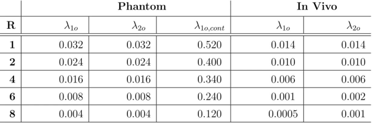
Table 2.1: Reconstruction Parameters Phantom In Vivo R λ1o λ2o λ1o,cont λ1o λ2o 1 0.032 0.032 0.520 0.014 0.014 2 0.024 0.024 0.400 0.010 0.010 4 0.016 0.016 0.340 0.006 0.006 6 0.008 0.008 0.240 0.001 0.002 8 0.004 0.004 0.120 0.0005 0.001

Reconstruction parameters for phantom and in vivo data at various accelera-tion factors (R). λ1 = 10λ1o for CShigh, λ1 = λ1o,cont for CScont, and λ1 = λ1o

for all remaining reconstructions. λ2 = λ2o for all reconstructions. With this

selection, TCS reconstructions scaled the `1-norm penalty from 10λ1o in

back-ground to λ1o in vessels, and the TV penalty from λ2o in background to λ2o/10

in vessels.

on a spatial weight map derived from vessel segmentations. The binary segmen-tations indicate the location of vessels across the imaging volume. To improve robustness against segmentation errors and partial volume effects near the vessel boundaries, segmentations were dilated by one pixel in all dimensions and linearly ramped down from 1 to 0 across the dilated region. The maps were subtracted from 1 and normalized to calculate W (i, j) that decreased from r (r ≥ 1) to 1. This spatial map was then used to modify the penalty weights as follows:

λ1(i, j) → λ1W (i, j) (2.5)

λ2(i, j) → λ2W (i, j)/r (2.6)

To improve background suppression, the `1-norm penalty weights were scaled

from rλ1 in background regions to λ1 in vessels. To minimize vessel loss, the TV

penalty weights were scaled from λ2in background regions to λ2/r in vessels. The

value of r was selected to maximize image contrast without introducing significant image distortions.

2.2.4.4 Phantom and in vivo reconstructions

For each dataset, separate Fourier (ZF), conventional CS and targeted CS (TCS) reconstructions were computed using parameters listed in Table 2.1. For ZF, data were compensated for k-space sampling density and inverse Fourier transformed. For CS, an identical λ2 = λ2o was prescribed but several different λ1 values were

used. First conservative CS was performed using λ1 = λ1o (CSlow). Second

heav-ier penalization was performed using λ1 = 10λ1o (CShigh). For phantom datasets,

a separate CS was calculated with an even larger λ1 = λ1o,cont (CScont), where

λcont was selected to attain identical blood/background contrast to TCS. Because

CScont caused severe image artifacts, it was omitted in subsequent analyses.

TCS was performed using λ1,2 = λ1o,2o and r ∈ [1 20]. For comparison, four

other spatially-adaptive CS methods were employed with the same parameters. First an intensity-weighted reconstruction was performed using weight maps de-rived from the intensity of ZF (CSint). ZF reconstructions were normalized to

a maximum amplitude of unity and then inverted to calculate W (i, j) similar to TCS. Second, iteratively-reweighted CS (CSIR) was performed [61]. Weight

maps for CSIR were updated at each iteration based on the reconstruction at the

previous iteration. Unlike TCS or CSint, CSIR maps did not reflect the region

of signal support but rather the intensity of reconstructed images [61]. Finally, two separate variants of the TCS method were implemented to assess the relative importance of using spatially-adaptive weights on TV versus `1 penalties. The

first variant TCSnT V employed a spatially-weighted `1 and a fixed TV penalty,

whereas the second variant TCSn`1 employed a spatially-weighted TV and a fixed

`1 penalty.

2.2.5

Simulations

To evaluate TCS independently from segmentation, we created two numerical phantoms that contained vessels immersed in a block of muscle tissue (Fig. 3.3a,c).

Both tissues were modeled with circular cross-sections. The first phantom con-tained 25 vessels of diameters ranging from 0.33 mm (1 pixel) to 2 mm (6 pixels). The vessels were arranged on a 5×5 rectilinear grid within a muscle block of diameter 100 mm (300 pixels). The second phantom contained 13 vessels of di-ameters between 1.25 to 3.75 mm, arranged randomly within the muscle block. Blood and muscle signals were simulated with the following parameters: α = 60o, TRl,s = 3.45/1.15 ms, TE = 1.725 ms, T1/T2 = 1200/200 ms for blood [62] and

870/50 ms for muscle [5]. The phantom images were sampled with a 384×384 grid over a 128×128-mm2 _{field-of-view. Circular cross-sections were created with}

a Fermi window using 1 pixel transition width. Finally, white Gaussian noise was added to yield a blood SNR of 20.

To examine penalty parameters used in TCS, we undersampled images of the first phantom with acceleration factors R = 1, 2, 4, 6 and 8. For each R, λ1,2

values were ranged between 0 to 2 times the λ1o,2o values listed in Table 2.1.

Meanwhile, the ratio (r) was varied in the range [1 20]. Larger TCS penalty weights yield improved background suppression (i.e., blood/muscle contrast), but cause distorted reconstructions of background signals. To assess reconstruction quality, a performance metric was calculated as the proportion of relative contrast difference to relative distortion level. Contrast improvement for each vessel was taken as:

% difference = ₁ContT CS− ContZF

2(ContT CS + ContZF)

× 100 (2.7)

Distortion level was taken as the normalized dispersion index of background tis-sue,

∆D = DIT CS DIZF

(2.8) where DI = σ2_{/µ, and µ, σ denote the mean and standard deviation of the muscle}

signal, respectively.

TCS performance was assessed as a function of r (Fig. 3.3b), when λ1,2 = λ1o,2o.

Performance increases rapidly as r is initially raised above 1, and it saturates for relatively large r. Note that higher r enhances blood/background contrast at the expense of increased image distortions. Thus, for all R, r = 10 was selected that maintains more than 80% of the optimal performance. We then inspected

the performance for r = 10, λ1 = nλ1o and λ2 = nλ2o with n varying in the

range [0 2]. Near optimal performance is attained for λ1,2 = λ1o,2o. Independent

optimizations of penalty weights indicate that λ1,2 = λ1o,2oand r = 10 yield close

to optimal performance for CSint,IR as well. Therefore, they were prescribed

for all reconstructions hereafter. To examine the effects of vessel size, TCS was calculated for 20 independent instances of additive noise. As expected, smaller vessels -more susceptible to signal loss– exhibit greater contrast improvement with TCS.

Next, we assessed the benefits of TCS on the second phantom closely mimicking vessel sizes in the extremities [63]. Blood/muscle contrast and spatial resolution were compared across CS and TCS (Fig. 3.3c). Spatial resolution was taken as the FWHM sizes of individual blood vessels normalized by the prescribed sizes in the numerical phantom. Statistical differences were assessed with Wilcoxon signed-rank tests.

To investigate robustness against segmentation errors, separate TCS re-constructions were performed by simulating losses in segmented vessel maps (Fig. 3.3d). The ideal vessel masks were eroded to yield a volumetric loss varying between 0-30% of the total vessel volume. The erosion process used a random voxel selection that maintained spatial contiguity for each vessel. TCS was calcu-lated for 20 distinct instances of vessel erosion and additive noise. Blood/muscle contrast and normalized vessel sizes were measured for each vessel individually and then averaged across 13 vessels.

Figure 2.4: (a) A phantom with 25 blood vessels of sizes 0.33 to 2 mm enclosed by muscle. Targeted CS (TCS) reconstructions were calculated using r ∈ [1 20], λ1,2 = λ1o,2o, and R = 1-8. Results are shown for R = 4, with magnified

lower-right portions of images. Higher r enhance blood/muscle contrast, but image distortions become prominent for r ≥ 15. (b) TCS performance was taken as the ratio of contrast improvement to dispersion level (mean±sem across vessels). For all R, r = 10 and λ1,2 = λ1o,2o yield close to optimal reconstruction performance

(left and middle panels). TCS using λ1,2 = λ1o,2o and r = 10 was repeated for

20 random instances additive noise. Contrast improvement is plotted for each vessel diameter (right panel; mean±sem across 20 images). The improvement is greater for smaller vessels. (c) A separate phantom with 13 blood vessels of sizes 1.25 to 3.75 mm. Fourier reconstructions (ZF), conventional CS, and TCS were calculated for R = 4. The panel below each image shows a sample line profile (across the red line). TCS improves blood/muscle contrast without significant image distortions. (d) TCS reconstructions were obtained while losses in segmented vessel maps were simulated by random erosions of the ideal map. Contrast and vessel sizes were measured relative to a TCS reconstruction based on the ideal map (mean±sem across 20 instances of erosion).

2.2.6

Experiments

To demonstrate TCS, we first acquired in vivo hand and lower-leg angiograms on a 1.5 T GE Signa EX scanner with CV/i gradients (maximum strength of 40 mT/m and slew rate of 150 T/m/s). High-resolution hand angiograms were collected in a healthy subject (male, age 27) using an 8-channel receive-only knee array, and with the following parameters: 0.5×0.5×0.5-mm3 spatial resolution, 320×240×120 encoding matrix, α = 60o, TRl,s = 3.6/1.2 ms, TE = 1.8 ms,

125-kHz readout bandwidth, 80-ms T2-preparation, 10-tip linear ramp

catalyza-tion, 10 k-space segments, 4-s intersegment recovery time, and a total scan time of 3 min 40 s. Hand angiograms were retrospectively undersampled by accel-eration factors of R = 1 (fully-sampled), 2, 4, 6 and 8. Data from each coil were reconstructed individually and sum-of-squares combined [64]. Meanwhile, prospectively undersampled lower-leg angiograms were collected in a healthy sub-ject (female, age 28) using a transmit-receive quadrature extremity coil, and with identical parameters to the hand protocol except for: 1×1×1-mm3 _spatial

reso-lution, 192×128×128 encoding matrix, TRl,s = 3.45/1.15 ms, TE = 1.725 ms.

Separate acquisitions were performed at R = (1,2,4,6,8) with number of mag-netization preparations N = (4,16,22,24,26) respectively, and scan time for each acquisition was 1 min 30 sec.

To validate TCS results in a broader population, we next collected lower-leg angiograms from 4 healthy subjects (1 female, 3 males; ages 27-32) and foot angiograms from 4 healthy subjects (2 females, 2 males; ages 27-30). Data were acquired on a 1.5 T GE Signa EX scanner using a quadrature extremity coil, with identical parameters to the lower-leg protocol listed above. The only exception was a fixed number of magnetization preparations N = 4 for all accelerations.

Vasculature maps were extracted from ZF reconstructions of undersampled data. CS and TCS reconstructions were then calculated on 2D cross sections. Reconstruction parameters were selected by examining TCS performance as a function of r and λ1,2. It was observed that near-optimal performance is obtained

for r = 10 and λ1,2 = λ1o,2o. To minimize partial volume effects in

maximum-intensity projection (MIP) views, all reconstructed datasets were upsampled by a factor of two in all dimensions by zero-padding in k-space.

To assess image contrast, average blood and muscle signals were measured in 13 coronal cross-sections spanning across the entire volume. Within a single section, two separate regions-of-interest (ROIs) with homogeneous blood and muscle sig-nal were selected. Sigsig-nals were averaged within these ROIs, and ratio of blood to muscle signal was taken as the contrast for each cross-section. ROIs were identical across reconstructions of the same anatomy. In hand angiograms, blood signal was measured on superficial to deep segments of digital radial and ulnar arteries (569±142 voxels, mean±s.d. across 13 cross sections), muscle signal was mea-sured in the palmar region (473±68 voxels). In lower-leg angiograms, blood signal was measured on proximal to distal segments of the tibial and peroneal arteries (73±20 voxels), muscle signal was measured across neighboring tissue (101±20). In foot angiograms, blood signal was measured on dorsal metatarsal and plan-tar arteries (52±34 voxels), and muscle signal was measured across neighboring tissue (80±29).

To examine potential blurring artifacts, vessel thickness measurements were performed in hand and lower leg datasets. For this analysis, vessels of various sizes were selected across 10 different axial cross-sections. The thickness of each vessel was taken as the diameter of the FWHM region, which ranged from 1 to 4 mm. The level of blurring in each reconstruction method was calculated as the relative vessel diameter compared to a ZF reconstruction of fully-sampled data (R = 1).

Two expert radiologists evaluated the diagnostic quality of reconstructed im-ages by consensus. At each R, MIP views were used to compare imim-ages from different reconstruction methods (without method identifiers). Image contrast, vessel demarcation and distal-branch visualization in each image were separately rated using a five point scale (5 excellent, 4 good, 3 moderate, 2 limited, 1 poor). Statistical differences in quantitative measurements and rating scores were as-sessed with Wilcoxon signed-rank tests.

2.3

Results

Blood/muscle contrast and resolution on simulated phantom images are listed in Table 2.2. At each R, TCS significantly improves contrast compared to all other methods including TCSnT V and TCSn`1 (P < 0.05). We find an improvement

of 21.5±8.7% over CSlow (mean±s.d. across R) and 11.3±2.8% over CSIR, the

closest CS competitor to TCS. The contrast improvement is greater for lower R values, where heavier sparsity penalties can be enforced due to increased acqui-sition SNR. Furthermore, TCS maintains improved spatial resolution compared to other CS methods and TCSn`1 at each R (P < 0.05). This improvement in

resolution is more prominent in higher R datasets that are more susceptible to resolution loss.

To assess the reliability of TCS against segmentation errors, phantom images were reconstructed for varying volumetric losses in vessel maps. TCS using ran-domly eroded versions of the ideal vessel map was compared to TCS using the ideal map (Fig. 3.3d). At all R values, contrast remains within 8% and vessel size remains within 12% of their ideal values for up to 30% segmentation loss. These results indicate that TCS shows considerable performance in the presence of moderate segmentation errors.

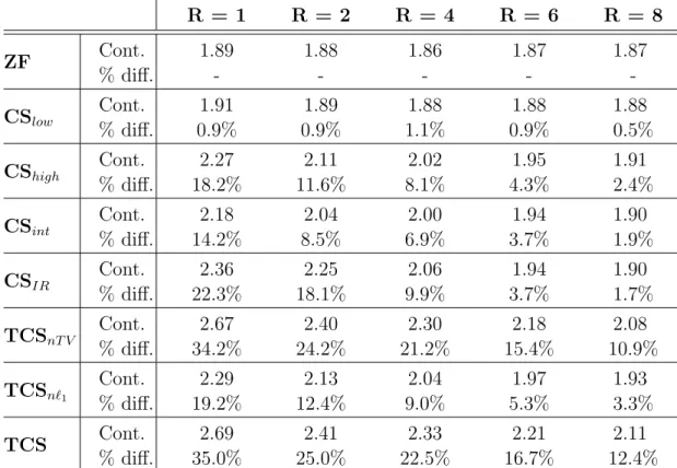
Table 2.2: Contrast and Resolution: Simulated data Contrast R = 1 R = 2 R = 4 R = 6 R = 8 ZF Cont. 1.89 1.88 1.86 1.87 1.87 % diff. - - - - -CSlow Cont. 1.91 1.89 1.88 1.88 1.88 % diff. 0.9% 0.9% 1.1% 0.9% 0.5% CShigh Cont. 2.27 2.11 2.02 1.95 1.91 % diff. 18.2% 11.6% 8.1% 4.3% 2.4% CSint Cont. 2.18 2.04 2.00 1.94 1.90 % diff. 14.2% 8.5% 6.9% 3.7% 1.9% CSIR Cont. 2.36 2.25 2.06 1.94 1.90 % diff. 22.3% 18.1% 9.9% 3.7% 1.7% TCSnT V Cont. 2.67 2.40 2.30 2.18 2.08 % diff. 34.2% 24.2% 21.2% 15.4% 10.9% TCSn`1 Cont. 2.29 2.13 2.04 1.97 1.93 % diff. 19.2% 12.4% 9.0% 5.3% 3.3% TCS Cont. 2.69 2.41 2.33 2.21 2.11 % diff. 35.0% 25.0% 22.5% 16.7% 12.4% Resolution R = 1 R = 2 R = 4 R = 6 R = 8 ZF 1.09±0.05 1.12±0.06 1.27±0.14 1.36±0.21 1.42±0.29 CSlow 1.05±0.04 1.08±0.05 1.09±0.06 1.08±0.06 1.17±0.09 CShigh 1.06±0.05 1.09±0.06 1.10±0.07 1.09±0.06 1.15±0.10 CSint 1.07±0.04 1.11±0.06 1.17±0.09 1.16±0.08 1.18±0.12 CSIR 1.07±0.04 1.06±0.05 1.16±0.08 1.18±0.08 1.20±0.12 TCSnT V 1.00±0.01 1.01±0.02 1.00±0.01 0.99±0.01 0.99±0.02 TCSn`1 1.05±0.04 1.08±0.05 1.09±0.05 1.06±0.05 1.12±0.08 TCS 1.00±0.01 1.01±0.01 1.00±0.01 0.98±0.02 0.98±0.02 Contrast: Average blood/muscle contrast on phantom data at various R. Raw contrast values are listed together with the percentage difference in contrast between each method and ZF. Resolution: Relative radius of blood vessels in phantom images (mean±s.d. across 13 vessels) compared to the actual vessel sizes.

Representative reconstructions of in vivo hand and lower-leg angiograms are shown in Figs. 2.5-2.7. TCS visibly improves blood/background contrast and enhances vessel depiction via tailored penalty weights. Note that we find no sig-nificant differences in vessel thickness across reconstructions methods and across R (P > 0.125). Thus the prominent appearance of vessel trees in TCS reconstruc-tions is due to improved angiographic contrast. While some small vessels are less effectively visualized at R ≥ 6 due to reduction of segmented volumes (Fig. 2.3), TCS reliably depicts major vessels including the digital-radial/ulnar arteries in the hand, and popliteal/peroneal arteries in the lower leg. Blood/background con-trast measurements in representative hand and lower-leg angiograms are listed in Table 2.3 and Table 2.4. At each R, TCS yields significantly higher contrast than all other methods including TCSnT V and TCSn`1 (P < 0.05). In the hand, the

improvement is 71.3±28.9% over CSlow and 33.0±6.6% over CSIR. In the lower

leg, the improvement is 38.5±8.5% over CSlow and 22.1±6.6% over CSIR.

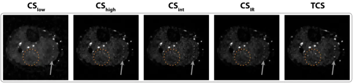
CS_low CS_high CS_int CS_IR TCS

Figure 2.5: Lower-leg angiograms reconstructed using conventional CS with uniformly-weighted penalty terms (CSlow, CShigh), CS with spatially-weighted

penalty terms based on intensity of ZF reconstructions (CSint),

iteratively-reweighted CS (CSIR), and TCS. Representative axial sections are shown for

R = 4. CShigh, CSint and CSIR suffer from signal losses, particularly in relatively

small or low intensity vessels. In contrast, TCS improved background suppres-sion while preserving detailed depiction of vasculature (marked with ellipses and arrows).

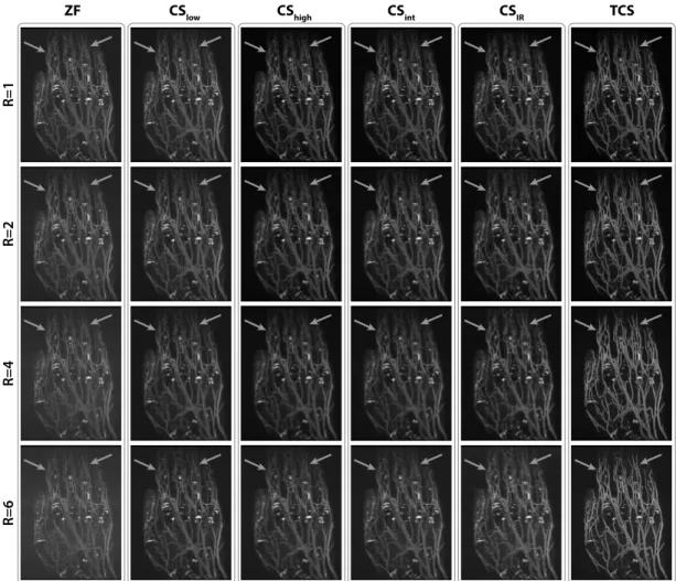
ZF CS_low CS_high CS_int R=1 R=2 R=4 R=6 CS_IR TCS

Figure 2.6: MIPs of hand angiograms reconstructed with ZF, CSIR and TCS,

for R = 1-6. CSIR suffers increasingly from loss of small vessels for higher R.

Furthermore, bright synovial fluid causes suboptimal vessel contrast in ZF and CSIR. In contrast, TCS alleviates vessel loss while improving suppression of

ZF CS_low CS_high CS_int R=1 R=2 R=4 R=6 CS_IR TCS

Figure 2.7: MIPs of lower leg angiograms reconstructed with ZF, CSIR and TCS,

for R = 1-6. There is visible loss of low-intensity and small vessels in CSIR.

TCS achieves improved blood/muscle contrast with no visible vessel loss up to R = 4 (marked with ellipses). Due to reduction of segmented volumes for R = 6 (Fig. 2.3), some small vessels are depicted suboptimally.

The contrast measurements in lower-leg and foot angiograms collected in a population of 8 subjects are listed in Table 2.5 and Table 2.6. Across subjects, TCS achieves higher contrast than all other reconstructions at each R (P < 0.05). In the lower leg, the improvement is 30.6±11.3% over CSlow, 13.8±2.7%

over CSIR, 3.0±1.4% over TCSnT V and 13.8±2.7% over TCSn`1. In the foot,

TCSnT V and 11.4±2.6% over TCSn`1. Consistent with simulation results, contrast

improvement for in vivo data is greater for lower R.

Radiological assessments of image contrast, vessel demarcation, and distal-branch visualization concur that the proposed method enhances image quality (see Table 2.7). Across all subjects, TCS achieves higher image contrast and vessel demarcation scores than all other CS reconstructions at each R (P < 0.05), except for R = 1 where we find no significant difference. While comparisons are less uniform for distal-branch visualization, the average visualization score across R is higher for TCS compared to all other reconstructions (P < 0.05).

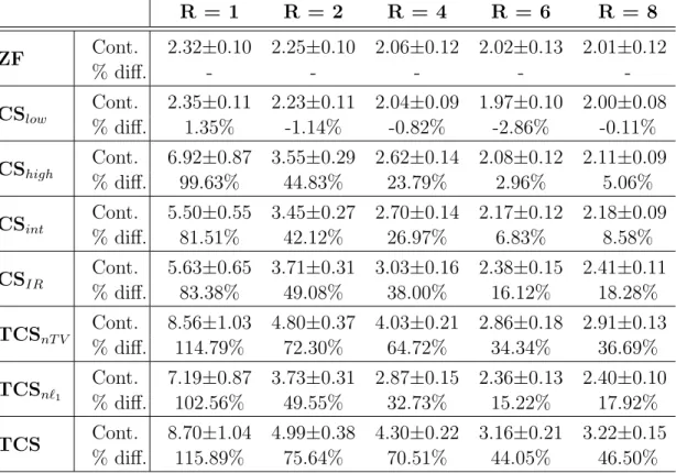
Table 2.3: Contrast: Representative Single-Subject Hand Data R = 1 R = 2 R = 4 R = 6 R = 8 ZF Cont. 2.32±0.10 2.25±0.10 2.06±0.12 2.02±0.13 2.01±0.12 % diff. - - - - -CSlow Cont. 2.35±0.11 2.23±0.11 2.04±0.09 1.97±0.10 2.00±0.08 % diff. 1.35% -1.14% -0.82% -2.86% -0.11% CShigh Cont. 6.92±0.87 3.55±0.29 2.62±0.14 2.08±0.12 2.11±0.09 % diff. 99.63% 44.83% 23.79% 2.96% 5.06% CSint Cont. 5.50±0.55 3.45±0.27 2.70±0.14 2.17±0.12 2.18±0.09 % diff. 81.51% 42.12% 26.97% 6.83% 8.58% CSIR Cont. 5.63±0.65 3.71±0.31 3.03±0.16 2.38±0.15 2.41±0.11 % diff. 83.38% 49.08% 38.00% 16.12% 18.28% TCSnT V Cont. 8.56±1.03 4.80±0.37 4.03±0.21 2.86±0.18 2.91±0.13 % diff. 114.79% 72.30% 64.72% 34.34% 36.69% TCSn`1 Cont. 7.19±0.87 3.73±0.31 2.87±0.15 2.36±0.13 2.40±0.10 % diff. 102.56% 49.55% 32.73% 15.22% 17.92% TCS Cont. 8.70±1.04 4.99±0.38 4.30±0.22 3.16±0.21 3.22±0.15 % diff. 115.89% 75.64% 70.51% 44.05% 46.50% Blood/muscle contrast (mean±s.d. across 13 sections) in hand angiograms at various R. Raw contrast values are listed together with the percentage difference in contrast between each method and ZF.

Table 2.4: Contrast: Representative Single-Subject Lower Leg Data R = 1 R = 2 R = 4 R = 6 R = 8 ZF Cont. 1.82±0.24 2.11±0.27 2.24±0.14 2.61±0.18 2.74±0.20 % diff. - - - - -CSlow Cont. 1.84±0.27 2.13±0.32 2.31±0.20 2.66±0.20 2.72±0.32 % diff. 1.06% 1.08% 2.95% 2.06% -0.49% CShigh Cont. 2.52±0.59 2.68±0.57 2.71±0.31 2.79±0.24 2.81±0.41 % diff. 31.90% 23.83% 19.18% 6.67% 2.79% CSint Cont. 2.46±0.48 2.69±0.55 2.79±0.30 2.85±0.20 2.85±0.28 % diff. 29.66% 24.36% 22.05% 8.91% 4.19% CSIR Cont. 2.50±0.58 2.74±0.59 2.77±0.36 2.87±0.28 2.79±0.45 % diff. 31.24% 26.22% 21.29% 9.47% 1.80% TCSnT V Cont. 3.04±0.69 3.11±0.65 3.28±0.39 3.30±0.31 3.57±0.50 % diff. 50.03% 38.46% 37.84% 23.37% 26.51% TCSn`1 Cont. 2.57±0.60 2.76±0.58 2.84±0.32 2.99±0.27 3.10±0.45 % diff. 34.11% 26.72% 23.70% 13.65% 12.58% TCS Cont. 3.11±0.70 3.17±0.65 3.42±0.40 3.52±0.34 3.88±0.54 % diff. 52.08% 40.28% 41.62% 29.76% 34.63% Blood/muscle contrast (mean±s.d. across 13 sections) in lower leg angiograms at various R. Raw contrast values are listed together with the percentage difference in contrast between each method and ZF.

Table 2.5: Contrast: Population Lower Leg Data R = 1 R = 2 R = 4 R = 6 R = 8 ZF Cont. 2.19±0.28 2.17±0.28 2.12±0.27 2.08±0.25 2.04±0.25 % diff. - - - - -CSlow Cont. 2.21±0.29 2.17±0.30 2.10±0.30 2.05±0.29 2.02±0.31 % diff. 1.2±0.8% -0.1±1.3% -1.1±2.0% -1.9±2.9% -1.4±4.1% CShigh Cont. 2.99±0.43 2.68±0.38 2.39±0.37 2.12±0.31 2.07±0.31 % diff. 30.8±6.2% 20.7±3.5% 11.6±3.2% 1.7±3.4% 1.3±3.9% CSint Cont. 3.00±0.58 2.71±0.44 2.41±0.41 2.13±0.32 2.08±0.32 % diff. 30.6±8.7% 21.5±4.5% 12.4±4.5% 2.0±3.6% 1.5±4.0% CSIR Cont. 3.02±0.48 2.76±0.42 2.50±0.43 2.14±0.32 2.08±0.32 % diff. 31.7±7.3% 23.6±5.3% 15.8±4.7% 2.7±3.9% 1.9±4.1% TCSnT V Cont. 3.41±0.45 3.10±0.38 2.87±0.36 2.37±0.30 2.34±0.29 % diff. 43.6±8.8% 35.2±5.9% 30.0±3.8% 12.9±3.4% 13.8±3.7% TCSn`1 Cont. 3.03±0.44 2.73±0.37 2.48±0.37 2.21±0.30 2.17±0.30 % diff. 32.4±6.6% 22.8±4.3% 15.2±2.9% 6.0±3.0% 6.1±3.3% TCS Cont. 3.46±0.45 3.15±0.36 2.97±0.35 2.47±0.29 2.45±0.28 % diff. 45.0±8.1% 36.9±6.6% 33.4±4.6% 17.0±3.9% 18.5±4.2% Blood/muscle contrast (mean±s.d. across 4 subjects) in lower-leg angiograms at various R. Raw contrast values are listed together with the percentage difference in contrast between each method and ZF.

Table 2.6: Contrast: Population Foot Data R = 1 R = 2 R = 4 R = 6 R = 8 ZF Cont. 2.45±0.23 2.41±0.20 2.31±0.19 2.21±0.16 2.08±0.15 % diff. - - - - -CSlow Cont. 2.49±0.23 2.44±0.24 2.35±0.26 2.27±0.26 2.18±0.27 % diff. 1.7±0.2% 1.1±1.5% 1.6±4.3% 2.2±5.1% 4.7±6.8% CShigh Cont. 3.21±0.28 2.98±0.21 2.71±0.27 2.39±0.27 2.29±0.29 % diff. 27.2±3.3% 21.0±3.7% 15.9±5.4% 7.2±5.6% 9.3±7.2% CSint Cont. 3.25±0.22 3.06±0.17 2.79±0.17 2.44±0.21 2.34±0.22 % diff. 28.4±4.6% 23.8±5.2% 19.1±5.1% 9.7±4.8% 12.0±5.2% CSIR Cont. 3.41±0.19 3.14±0.17 2.83±0.18 2.45±0.21 2.34±0.25 % diff. 33.1±5.0% 26.3±6.7% 20.6±5.8% 10.1±5.0% 11.6±6.3% TCSnT V Cont. 3.49±0.29 3.30±0.18 3.18±0.17 2.65±0.23 2.58±0.27 % diff. 35.2±4.6% 31.1±6.7% 31.9±6.5% 17.9±6.4% 21.3±7.3% TCSn`1 Cont. 3.25±0.28 3.03±0.20 2.79±0.25 2.49±0.25 2.40±0.27 % diff. 28.1±3.9% 22.8±4.2% 18.9±5.5% 11.6±5.7% 14.4±6.8% TCS Cont. 3.54±0.30 3.37±0.17 3.26±0.16 2.76±0.23 2.71±0.26 % diff. 36.6±5.1% 33.1±6.6% 34.4±7.4% 22.0±7.4% 26.3±8.0% Blood/muscle contrast (mean±s.d. across 4 subjects) in foot angiograms at various R. Raw contrast values are listed together with the percentage differ-ence in contrast between each method and ZF.

Table 2.7: Radiological Assessment of Image Quality Image Contrast R = 1 R = 2 R = 4 R = 6 R = 8 ZF 4.1±0.1 4.1±0.1 3.5±0.2 2.7±0.2 2.1±0.2 CSlow 4.1±0.1 4.1±0.1 3.9±0.1 3.4±0.2 3.1±0.2 CShigh 4.5±0.2 4.1±0.2 3.6±0.2 3.4±0.2 3.1±0.2 CSint 4.4±0.2 3.9±0.2 3.2±0.3 3.0±0.3 2.8±0.3 CSIR 4.4±0.2 3.9±0.2 3.4±0.3 3.3±0.2 3.1±0.2 TCS 4.8±0.1 4.8±0.2 4.7±0.2 4.2±0.2 4.1±0.2 Vessel Demarcation R = 1 R = 2 R = 4 R = 6 R = 8 ZF 4.6±0.2 4.3±0.3 3.5±0.3 3.2±0.3 2.5±0.4 CSlow 4.6±0.2 4.4±0.2 3.7±0.2 3.3±0.3 2.5±0.2 CShigh 4.7±0.2 4.5±0.2 3.8±0.2 3.3±0.3 2.6±0.2 CSint 4.6±0.2 4.4±0.2 3.7±0.2 3.2±0.3 2.4±0.3 CSIR 4.6±0.2 4.5±0.2 3.8±0.2 3.2±0.3 2.5±0.2 TCS 5.0±0.0 5.0±0.0 4.9±0.1 4.4±0.2 3.9±0.2 Distal-Branch Visualization R = 1 R = 2 R = 4 R = 6 R = 8 ZF 4.6±0.2 4.5±0.2 3.7±0.2 2.9±0.3 2.2±0.3 CSlow 4.6±0.2 4.6±0.2 3.9±0.2 3.6±0.3 3.0±0.2 CShigh 4.3±0.2 4.4±0.2 3.5±0.2 3.6±0.3 3.0±0.2 CSint 4.3±0.2 4.3±0.2 3.3±0.2 3.4±0.3 2.9±0.2 CSIR 3.9±0.3 3.8±0.2 3.2±0.2 3.6±0.3 3.1±0.2 TCS 4.5±0.2 4.6±0.2 4.3±0.2 4.0±0.2 3.9±0.2 Rating scores for image contrast, vessel demarcation, and distal-branch visu-alization (mean±s.e.m. across 10 subjects).

2.4

Discussion

Here we propose a reconstruction strategy (TCS) for NCE angiograms that lever-ages vasculature maps extracted from undersampled data, without relying on prior information. The morphological information in these maps is used to apply order-of-magnitude heavier sparsity and TV penalties across background tissues compared to vessels. As such, TCS enhances blood/background contrast com-pared to conventional CS without degrading vessel depiction.

A recent study has used 2D segmentations to apply a spatially-varying `1

-penalty [49]. While this previous approach has similar motivations to TCS, our study differs in several important aspects. First, we use a tractographic segmenta-tion to exploit 3D structure and leverage vessel contiguity in the superior-inferior direction. Second, we utilize concurrent spatial-weighting on both `1-norm and

TV penalties to minimize vessel signal loss. Our results show that concurrent weighting in TCS enhances image quality over weighting either term alone. Lastly apart from noise/aliasing reduction aimed previously, here we demonstrate con-trast enhancement that significantly improves vessel depiction in concon-trast-limited NCE MRA.

Practical benefits of TCS depend on the coverage of the segmented vasculature maps. Our simulations suggest that TCS maintains considerable performance with up to 30% volume loss in segmented maps. However with increased alias-ing at high R, small vessels with low contrast may be missed and thereby incur heavy penalties during TCS. Here some small, low-contrast branches were not segmented at R = 6 and 8; and loss of high-spatial-frequency information in TCS became prominent at R = 8 (not shown). Such losses may mimic stenoses in mi-nor vessel branches. To minimize misassessment, segmented maps can be more broadly dilated and reconstruction penalties may be limited at higher R. Alterna-tively, segmentation and reconstruction stages can be cast as a joint optimization problem [65], with iterative refinement across both stages. These demanding op-timizations can be completed in practical run times using graphical processing units [66, 67].

With heavier undersampling, it will become challenging to distinguish vessel signals from aliasing/noise interference. Higher R can be attained for TCS by im-proving SNR, blood/background contrast and spatial resolution of angiographic acquisitions. These improvements will boost both segmentation and reconstruc-tion performances. Furthermore, increased spatial resolureconstruc-tion can also enhance the delineation of vessel boundaries during segmentation. Here we prescribed relatively high spatial resolution (e.g. 0.5 mm for hand), and used a segmenta-tion that can detect a minimum lumen size equal to this resolusegmenta-tion. However, delineation of small, distal vessels might be impaired at more limited spatial res-olutions. In such cases, parallel imaging and CS techniques can be combined to alleviate resolution limitations [9, 68].

TCS applies first-order finite difference operators to incur a TV penalty. Penalty weights were kept low here to minimize block artifacts, and no signif-icant distortions were observed around vessels. However, higher-order TV terms may enable better denoising in piece-wise smooth regions while preserving edge information near vessel boundaries [69]. Another improvement for TCS concerns the sparsity penalties applied in the image domain. While angiographic images are natively sparse, spatially-weighted penalties in relevant sparsifying transform domains (e.g. wavelet domain) might be needed for other applications. Adaptive wavelet-domain penalties have been previously designed based on manual ROI specifications [46] or dependencies between wavelet coefficients [70]. Similarly, TCS with spatially-weighted wavelet penalties may be useful in applications such as coronary imaging.

Residual signals from several background tissues are evident in FIA datasets. First, synovial fluid in the joints with relatively high T2/T1 ratio yields

compa-rable bSSFP signal to vessels. While our segmentations correctly classify syn-ovial fluid as background, excessive reconstruction penalties are required to fully dampen these bright signals. If further suppression is desired, synovial fluid maps can be manually segmented to apply higher penalty weights compared to other background tissues. Second, the vessel maps presented here contain both arte-rial and venous streams in the peripheral extremities. Because the two streams may be located closely, segmentation algorithms can assign venous voxels onto