The role of ecological footprint and the changes in degree days on
environmental sustainability in the United States
Seyi Saint AKADIRI
11 Research Development, Central Bank of Nigeria, Abuja, Nigeria
E-mail: [email protected]
Andrew Adewale ALOLA*
2, 32 Department of Economics,
Faculty of Administrative and Social Science Istanbul Gelisim University, Istanbul, Turkey
3Department of Financial Technologies, South Ural State University, Chelyabinsk, Russia
*E-mail: [email protected]
Uju Violet ALOLA
4, 54 Department of Tourism Guidance,
Istanbul Gelisim University, Istanbul, Turkey
5 School of Economics and Management
South Ural State University, Lenin prospect 76, Chelyabinsk, 454080, Russian Federation E-mail: [email protected]
Chioma Sylvia NWAMBE
66 Department of Economics,
Eastern Mediterranean University, KKTC, Turkey E-mail: [email protected]
Abstract
In addition to the adverse effect of extreme weather and weather variation across the globe, the ecological deficit accounting associated with the United States is perceived to have further worsen the country’s environmental quality. Considering the aforementioned motivation, this study examined the effects of cooling degree days, heating degree days and ecological footprint on environmental degradation in the United States over the period of 1960 to 2016. While employing
the Autoregressive Distributed Lag (ARDL) and Bounds testing to cointegration approaches, the Gross Domestic Product (GDP) per capita is further incorporated in the estimation model to avoid estimation bias thus enhancing a robust estimate. The result overwhelmingly found that the cooling degree days, the heating degree days, and the ecological footprint accounting aggravates the country’s environmental degradation. Worse still, the study further presents that there is short-run adverse impacts of the heating and cooling degree-days, and the short-run and long-run ecological footprint on the country’s environmental sustainability. Moreover, there is statistical evidence that the income growth in the United States especially in the long-run will not also improve the environmental quality. Irrespective of the income-environmental degradation long-run relationship, the relieving impact of income growth on environmental degradation is observed in the short-run. In general, the study presents relevant policy pathway for implementation.
Keyword: environmental sustainability; cooling degree day; heating degree day; ecological footprint; United States.
1. Introduction.
Putting into perspective the outcomes and efforts of the United States Climate Alliance and its associated climate-oriented policies, the evidence of the country climate actions has not gone without notice. Resulting from the quest for investment in cleaner energy-saving technology, energy-efficiency production processes, and climate resilience actions, the effort has reportedly accounted for the reduction of greenhouse gas between 2005 and 2016 by about 14% as argued by the United States Climate Alliance (2019). In the light of this positive climate and environmental friendlier policies, there is need for, sound and productive weather-oriented policies that will
directly/indirectly put into consideration the adverse effect of the extreme weather conditions across the global.
The growing concern of global warming arising from the adverse weather variation and increasing push for economic dominance among the advanced nations especially the United States accounts for the vast interest in environmental-linked studies. On this note, the current study mainly examined the effect of the degree-days (the cooling and heating degree days) and the ecological footprint accounting of the United States on environmental degradation. While the study is important for the United States because of the vast deficit of ecological footprint of the country (Global Footprint Network, 2019), the United States is equally known to experience significant weather variation in the last decades.
The damaging effects of climate change have been of concern to the scientists, economists, governments, private institutions, individuals and policymakers. Recent occurrences around the globe have proven beyond doubt that science is absolutely right, the effects of climate change are upon us, even faster than the scientists had projected and predicted. The impacts are becoming increasingly obvious on a daily basis and it affecting almost animals and human in an increasingly ways. For example the erratic changes in weather conditions either in terms of cooling or heating degree-days have had one impact or another on the environment and a rise in climate change as a whole (Alola et al 2019a). The situation of the recent bush fire outburst in California and Australia are typical examples of the severe changes and unfriendly temperature has had on the animals and human in general. The lengthened global warming as a result of erratic changes in weather conditions had been associated with the severe and extreme drought and incessant fire outburst around the globe (Union of concerned Scientist, 2019).
The ecological footprint on the other hand take into consideration human needs on nature (Saint Akadiri et al, 2019) that is, the units of nature needed to sustain people and the entire nation at large (Wackernagel, Lin, Evans, Hanscom & Raven, 2019). As pointed out by the Global Footprint Network (2019) hence GFN, there are basically two factors that determine or drives ecological footprint of any nation, these includes; population and consumption. It is paramount to point out here that, the said human demand on nature could be tracked via an ecological accounting procedure. This accounting procedure contrast the biologically productive region available in the world with the productive region human make use for consumption purposes which summarily is a means of evaluating human effect on ecosystem as it shows the dependency ratio of human needs on natural capital. Following the GFN report, the world ecological footprint on average is reported to be 2.75 global hectares (measured in gha/person) and about 22.6 billion in aggregate, alongside the world bio-capacity of 1.63 gha/person, with world bio-capacity aggregate of 12.2 billion. This statistic generates world ecological deficit value of 1.1 gha/person, totaled 10.4 billion (GFN, 2016).
According to the GFN report, nations of the world that has more than 1.73 gha/person have low resources need which is not sustainable (GFN, 2019). Additionally, the ones with an ecological footprint less than 1.73 gha/person may also not be sustainable. Thus, the quality of ecological footprint may influence or lead to ecological degradation. Based on this fact, one will be right to conclude theoretically that, as population growth increases, human demand on nature in terms of consumption would increase, thus, having a damaging impact on the quality and sustainability of the environment. Since the inability of a nation to have an adequate ecological resources to serve its population ecological footprint needs would lead to ecological deficit which consequently would make such nation ecological debtor and vice versa. In addition to the adverse effect of
extreme weather and weather variation across the globe, the ecological deficit accounting associated with the United States is perceived to have further worsened the country’s environmental quality.
Considering the interactions between the variables under observation, this current study examined the effects of cooling degree-days (CDD), heating degree-days (HDD) and ecological footprint on environmental degradation in the case of the United States over the period 1960-2016. To achieve study objective of examining whether these variables has a short-run or long run impact on environmental degradation or not, we employ the Autoregressive Distributed Lag (ARDL) that generates short-run and long run estimates (even when the variables are partially integrated) and Bounds testing to cointegration approaches. We also incorporate (GDP) per capita in our CO2
emissions model to avoid estimation bias thus enhancing a robust estimate.
Summarily, based on our knowledge and especially in the case of the United States, this study is the first or among the few studies (if any) that uses a multivariate CO2 emissions model to examine
the impacts of ecological footprint, cooling degree days, heating degree days and real per capita income on environmental degradation. Thus, this study is an addition to energy-environmental sustainability study and policymaking. The current study posit that the cooling degree-days and the heating degree-days positively contribute to environmental degradation especially in the short-run. Although the long-run impacts are enormous, statistical evidence indicates that the impacts are not significant in the long run. However, the impact of the increasing demand of the country’s ecological footprint on environmental degradation is reportedly positive and significant both in the short- and long run. This further informs that there is a significant and adverse environmental hazard associated with the deficit accounting of the United States’ ecological footprint. Moreover, the environmental impact of income growth as observed in the result for the United States is
expected. The result posits that income growth in the United States especially in the long run would not damage the environmental quality.
The remaining section of this study is scheduled as follow: Section 2 briefly discussed the interaction between ecological footprint, cooling degree-days and heating degree-days and presentation of synopsis of extant studies. Section 3 is about the material, data description and adopted methods. While in section 4 we present results and discussed the results accordingly, section 5 concludes the study alongside policy suggestions.
2. Interaction of Ecological Footprint, Degree Days and the Environment
2.1 Conceptual frameworkLet us start the brief conceptual interactions between the variables under investigation by presenting the definition and the underlying concept of the degree-days i.e DD. The DD is the combination of temperature and time. In addition, the DD is the variance between the mean of daily temperature and the 65℉. This mean of daily temperature is calculated by dividing the summation of low temperature and higher temperature by 2. DD is built on the proposition that the cooling and/or heating are not required for human and animals comfortability when the outdoor temperature is 65℉ (Alola et al 2019a). According to the National Climatic Data Center (NCDC) 2019 report, in a situation where the mean of the daily temperature is lower than 65℉, we deduct the daily average temperature from 65℉ and the outcome would be the heating DD. Otherwise, if the mean of the daily temperature is higher than 65℉, we deduct the daily average temperature from 65℉ and the outcome would be the cooling DD (NCDC, 2019).
On the other hand, the temperature that is referred to here is treated as “changes in temperature” (i.e., delta (Δ) T), which is basically the variations between the base temperature and the outdoor
temperature. For better understanding, base temperature is solely the outdoor temperature that distinguishes a particular period when a building (either residential or commercial) requires cooling or heating from a period when the building does not needs the cooling or heating requirement. Based on this definition, it is inferred that if a base temperature is lower than the outdoor temperature, then heating needs should not be of a concern to sustain the required indoor temperature, and vice versa. Thus, we conclude that base temperature is a point of equilibrium (intersection) between the cooling and heating requirement of a building (NCDC), 2019).
2.2 Related Studies: A Synopsis
Although theoretical and qualitative studies have presented underlying concept of the nexus of degree days and environmental quality, until now only Alola et al 2019 and a few others have presented an empirical study on the subject. However, several studies have presented the determinants of environmental quality vis-à-vis environmental sustainability in different perspectives. For instance, existing literature has linked energy sources with environmental quality in different perspectives (Apergis & Payne, 2009; Ozturk & Acaravci, 2010; Apergis & Ozturk, 2015; Alola & Alola, 2018; Bekun, Emir & Sarkodie, 2019; Nathaniel & Iheonu, 2019; Adedoyin et al., 2020; Ike et al., 2020; Udi, Bekun & Adedoyin, 2020). Similarly, environmental quality has been linked with economic activities and expansion (Dogan, Seker & Bulbul, 2017; Udemba, 2019; Udemba, Güngör & Bekun, 2019; Nathaniel, Anyanwu & Shah, 2020), and other socioeconomic factors such as democracy, corruption, political institution, ICT, immigration and others (Solarin & Bello, 2018; Alola, 2019; Alola et al., 2019b; Ozturk, Al-Mulali & Solarin, 2019; Alola et al., 2020c; Saint Akadiri & Alola, 2020; Solarin & Bello, 2020; Usman, Iortile & Ike, 2020; Usman et al., 2020).
3.1 Material
It is paramount to state that, the most habitual use of DD statistic is for measuring the extent and level of energy consume as it will be impossible or inadequate to compare the extent or rate at which energy is used overtime without estimating the degree-days. For example, to examine whether the attic insulation injected into the fuel (to minimize energy usage) during the summer period eventually saved energy or not, one would need to compare the amount of cash saved via the disparity in the energy bills with and without the attic insulation injection (NCDC, 2019). Thus, variations in the level of energy consumed in any developing, emerging, and developed (industrialized) economies that rely on non-renewable energy source for consumption and production activities all over the year, and most particularly during the winter (for heating) and summer (for cooling) periods would impacts on the level of CO2 emissions, and hence
environmental degradation. In addition, the energy usage here is not only associated with weather conditions. It also put into considerations the household (residential) and commercial appliances, such as electricity, electric appliances, automobiles, and generators among others.
Additionally, since ecological footprint takes into consideration human needs on nature, then the impact of the units of nature needed to sustain people and the entire nation at large should be measured (Saint Akadiri et al 2019; Wackernagel et al 2019). These human needs of nature are basically determine by two of the factors: population and consumption. Therefore, it appropriate to deduce theoretically that an increase in population growth would increase demand for housing (building) and natural capital. These would in turn increase the level of energy usage for heating, cooling, transportation, and production purposes that facilitates economic growth. As consumption and productive activities stimulate growth, CO2 emissions increase, and hence increase in the level
Furthermore, it is presumed that the interaction between ecological footprint, cooling degree days, heating degree days and real per capita income directly or indirectly affect the level of environmental degradation. Specifically, this interaction is expected for the economies that experience increase in population growth and such that largely depends on non-renewables energy source for consumption and production activities. Thus, the presumed interaction result in socio-economic factor that drives world environmental pollution. Human needs are unlimited and resources (natural capital) to satisfy these unlimited wants are in limited supply (resulting in ecological deficit). Any attempt to coerce nature beyond its capacity via human efforts would continue to have damaging impacts on the environment either for the immediate and/or future generations.
3.2 Data Description
By considering the environmental impact of the drastic changes in the cooling and heating degree days1, the current investigation considered other potential determinants of environmental
sustainability. In so doing, the cooling degree days and heating degree days, the Gross Domestic Product per capita, and Ecological Footprint were employed as the independent variables. Additionally, the carbon dioxide emissions per capita is employed as the environmental sustainability variable for the investigation. The datasets were retrieved from different sources and spans over the period of 1960 to 2015. In Table 1, the variables employed, the unit of measurement and sources are further presented in details. The descriptive statistics and the line plot of the series are respectively presented as Table 2 and Figure 1.
Table 1: Variable description and measurement unit____________________________________
Indicator Name Abbreviation Measurement Scale Source
Carbon Emissions CE Metric tons per capita WDI
1The cooling and heating degree days for the United States (from the aggregate of 48 States, available in https://www.epa.gov/climate-indicators/climate-change-indicators-heating-and-cooling-degree-days).
Cooling Degree Days CDD Degree days USEPA
Heating Degree Days HDD Degree days USEPA
Ecological Footprint EFP Global hectares (GHA) EFP
Gross Domestic Product per capita GDP Constant 2010 US Dollars WDI
______________________________________________________________________________
Source: Authors’ computation.
Note: US EIA2,US EPA3and WDI4 represents the United States Environmental Protection Agency, United States
Energy Information Administration, and World Development Indicator respectively.
2https://www.eia.gov/totalenergy/data/browser/index.php?tbl=T10.01#/?f=M&start=200001 3 https://www.epa.gov/climate-indicators/climate-change-indicators-heating-and-cooling-degree-days
4https://data.worldbank.org/indicator. The more detail information on the description of the variables are available at
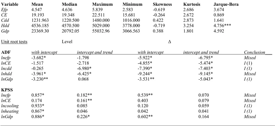
Table 2: Descriptive statistics and Unit root test with ADF and KPSS______________________________________________________________
Variable Mean Median Maximum Minimum Skewness Kurtosis Jarque-Bera
Efp 4.547 4.636 5.839 2.583 -0.619 2.686 3.674
CE 19.193 19.348 22.511 15.681 -0.264 2.672 0.869
Cdd 1231.963 1220.500 1480.000 1016.000 0.422 2.873 1.641
Hdd 4536.185 4570.500 5029.000 3778.000 -0.719 3.254 4.756** *
Gdp 23369.30 20792.05 55032.96 3066.563 0.388 1.801 4.592
Unit root tests Level Δ
ADF with intercept intercept and trend with intercept intercept and trend Conclusion___ lnefp -3.682* -1.798 -5.922* -6.795* Mixed lnCE -1.517 -2.718 -4.855* -5.474* I (1) lncdd -0.265 -6.980* -7.390* -7.403* I (1) lnhdd -3.961* -6.425* -9.244* -9.145* Mixed lnGdp -3.230** 0.068 -3.531** -5.043* I (1) KPSS lnefp 0.857* 0.182** 0.539** 0.070 Mixed lnCE 0.174 0.161** 0.403 0.079 Mixed lncooling 0.933* 0.085 0.120 0.059 I (1) lnheating 0.867* 0.046 0.042 0.041 I (1) lnGdp 0.886* 0.226* 0.602** 0.164 Mixed
Note: The ln, Level and Δ respectively indicates estimates of the natural logarithmic, level and the first difference. The lag selection is observed by SIC is 4 (lag=4)
for the ADF (Augmented Dickey-Fuller) and KPSS (using the Bartlett Kernel of Andrews automatic Bandwidth) unit root tests. *, ** and *** are the 1%, 5% and 10% statistical significance levels. Number of observation is 56. Moreover, the lgdp, lefp, lcdd, and lhdd are the respective logarithmic values of the Gross Domestics Product, Ecological Footprint, Cooling degree days, and Heating degree days across the United States for the investigated period 1960-2015.
2,800,000 3,200,000 3,600,000 4,000,000 4,400,000 4,800,000 5,200,000 5,600,000 6,000,000 60 65 70 75 80 85 90 95 00 05 10 15 CO2 (a) 0 10,000 20,000 30,000 40,000 50,000 60,000 60 65 70 75 80 85 90 95 00 05 10 15 GDP per capita (b)
Figure 1: The time plot of the variables; (a) is the carbon emissions (CE), (b)
is the Gross Domestic Product per capita, (c) is the Ecological Footprint (efp), (d) is the cooling degree days, and (e) is the cooling degree days.
2.5 3.0 3.5 4.0 4.5 5.0 5.5 6.0 60 65 70 75 80 85 90 95 00 05 10 15 Ecological Footprint (c) 1,000 1,100 1,200 1,300 1,400 1,500 60 65 70 75 80 85 90 95 00 05 10 15
Cooling Degree Days
(d) 3,600 3,800 4,000 4,200 4,400 4,600 4,800 5,000 5,200 60 65 70 75 80 85 90 95 00 05 10 15
Heating Degree Days
3.3. Methodology
3.3.1 Theoretical Framework
Given the goal of identifying the drivers of primary drivers of environmental degradation, the STIRPAT conceptual model (I = α Pb Ac Td e)5 has continued to play significant role and beyond the perspectives population (P), affluence (A), and technology (T). In the last decades, other factors are being investigated within the framework of environmental degradation and/or sustainability for different case studies (Alola, 2019; Alola, Bekun & Sarkodie, 2019; Alola & Kirikkaleli, 2019; Alola, Yalçiner & Alola, 2019; Alola et al., 2019a; Alola et al., 2019b; Bekun, Alola & Sarkodie, 2019; Saint Akadiri, Alola. & Akadiri, 2019; Saint Akadiri et al., 2019a; Saint Akadiri et al., 2019). Consequently, the current study follow the approach of Alola et al (2019a) that expressed the relationship between the degree days vis-à-vis the cooling and heating degree days, and the environmental sustainability. However, the current study underpins the role of changes in the biologically productive area (ecological footprint) and cooling and heating degree days on environmental quality. Therefore the environmental quality or sustainability is modelled herewith as
= ( , , , ) (1)
Consequently, for the data smoothing and easy interpretation of the results by using point elasticities, the expression (1) above is log transformed logarithmic transformation is given as:
= + + + + + (2)
5 Dietz, & Rosa (1994, 1997) had presented the determinants of carbon emissions in the framework of STIRPAT
(Stochastic Impacts by Regression on Population, Affluence and Technology) model. However, Ehrlich and Comnoner (1971) initially proposed the IPAT model to study the nexus of economic growth and environmental resources.
From the equation (2), 0 depicts the constant coefficient while the t is the period of analysis
ranging from 1960 to 2015. Also, represents the error term while , , ,, are the respective magnitude of the impact of income (Gross Domestic Product per capita), the ecological footprint (EFP), the cooling degree days (CDD), and the heating degree days (HDD) on environmental quality (Carbon emissions). Subsequently, the methods and discussions of the important tests such as the unit root and the short and long-run estimation are presented within the concept of equation (2).
3.3.2 Empirical Method
Before estimating the short and long-run from equation (2) especially with the Autoregressive Distributed Lag (ARDL) by Pesaran, Shin and Smith (2001), the stationarity of the variables is evaluated. The ADF-Augmented Dickey-Fuller (Dickey & Fuller, 1981) and KPSS (Kwiatkowski et al., 1992) are both employed respectively to evaluate the unit root and stationarity of the estimated variables. Because of space constraint, the step-by-step procedure of the ADF and the KPSS is not provided here but both results are illustrated in Table 2. Given that the variable are mixed order [i.e both I (0) and I (1)], the ARDL is found to be appropriate for the investigation. The ARDL is also appropriate at estimating either small or a large sample size dataste. Another reason for the use of the ARDL especially in the current case is it appropriateness to examine the short-run and long-run relationships. Therefore, the unrestricted Autoregressive Distributed Lag (ARDL) method for the equation (2) above is expressed as:
0 1 1 2 1 3 1 4 1
lnCE
t
lnGDP
t
lnEFP
t
lnCDD
t
lnHDD
t
1 1 2 1 3 1 4 1 0 0 0 0 lnCE lnGDP lnCDD lnHDD q q q q t t t t i i i i
t (3)while Δ is the difference operator, the λ0, … λ4 and θ0, … θ4 are the respective impacts of the
independent variables in the long-run and short-run respectively. This is because the first part of equation (3) is evaluates the long-run impacts (coefficients) while the second part of the equation (3) evaluates the short-run impacts (coefficients) of the independent variables on carbon emissions. Consequently, the bounds test to coingration approach of Pesaran, Shin and Smith (2001) is examined such that the null hypothesis of the test is given as
1
2
3
4
0
and the alternative is that
1
2
3
4
0
. Then, the null hypothesis H0 for these tests is given as0
:
0
H
against the alternative ofH
0:
0
.4. Empirical Result and Discussion
The descriptive statistics of the estimated variables (see Tables 2) provides a priori information that suggestively compliment the result of the relationship between the variables. Indicatively, the Jarque-Bera statistics indicates that all the variables except the heating degree days are normally distributed. Also, while the cooling degree days and GDP per capita are positively skewed, the CO2 emissions, heating degree days, and the ecological footprint are all negatively skewed.
Importantly, there is statistical evidence that are more heating degree days (peaked at 5029) than the cooing degree days (peaked at 1480). This evidence is further asserted by the significant difference in the minimum values of cooling and heating degree days, thus there is 2762 more heating degree days.
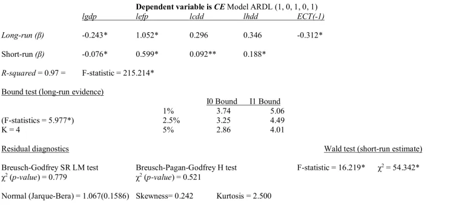
After employing the ARDL approach of Pesaran, Shin and Smith (2001) as described above, the results of the long and short-run, in addition with the bound test are presented in Table 3.
Table 3: ARDL-Bound Test_______________________________________________________________________________________ Dependent variable is CE Model ARDL (1, 0, 1, 0, 1)
lgdp lefp lcdd lhdd ECT(-1) Long-run (β) -0.243* 1.052* 0.296 0.346 -0.312* Short-run (β) -0.076* 0.599* 0.092** 0.188*
R-squared = 0.97 = F-statistic = 215.214* Bound test (long-run evidence)
I0 Bound I1 Bound
1% 3.74 5.06
(F-statistics = 5.977*) 2.5% 3.25 4.49
K = 4 5% 2.86 4.01
Residual diagnostics Wald test (short-run estimate)
Breusch-Godfrey SR LM test Breusch-Pagan-Godfrey H test F-statistic = 16.219* χ2 = 54.342*
χ2 (p-value) = 0.779 χ2 (p-value) = 0.521
Normal (Jarque-Bera) = 1.067(0.1586) Skewness= 0.242 Kurtosis = 2.500
______________________________________________________________________________________________________________________
Note: The Autoregressive Distributed Lad (ARDL) model employed is (1, 0, 1, 0, 1). Also, the p-value is the probability value and ECT is the Error Correction
Term. Similarly, the I0 and I1 are lower and upper bound of the bound test respectively, β is the estimate coefficient, χ2 is the Chi-square, SR LM is Serial correlation
Lagrange Multiplier and H is heteroskedasticity. Moreover, the lgdp, lefp, lcdd, and lhdd are the respective logarithmic values of the Gross Domestics Product, Ecological Footprint, Cooling degree days, and Heating degree days across the United States for the investigated period 1960-2015.
In essence, the evidence from Table 3 implies that both the cooling and heating degree days (respectively cdd and hdd) exerts positive and significant impacts on the carbon emissions per capita in the United States. The significant effect of the cdd and hdd on the CO2 emissions per
person are both positive in the short-run but with the heating degree days exerting more harmful impact (i.e 0.188% increase in per capita metric tons of CO2 against 0.092% for every 1% increase in the heating and cooling degree days respectively). Similarly, the heating degree days also exerts more harmful impact in the long-run than the cooling degree days, however both impacts are not statistically significant. The result opined that more consumption or tendency to consume more energy for heating purpose especially during the winter or cold season leads to more emission of carbon dioxide. In essence, the resulting effect is that the heating degree days is responsible for more severe environmental degradation. In affirming the result of the current study, Mutlu Ozturk, Dombayci and Caliskan (2019) found that maximum energy saving is found associated with lowest temperature which is the heating degree days. However, further studies have shown that the reverse (i.e the impact of climate change on the cooling and heating degree days) is equivalently valid (Li et al., 2009; Moustris et al., 2015; Li et al., 2018; Alola et al., 2019a).
Similarly, the impact of ecological footprint (efp) on environmental degradation vis-à-vis CO2
indicate that a one percent increase in efp is responsible for a significant 0.599% and 1.052% metric tons of CO2 in the short-run and long-run respectively. Indicatively, the study of Solarin
and Bello (2018) affirms that policy shock exerts significant impact on the ecological footprint. Interestingly, the impact of the Gross Domestic Product (gdp) per capita on environmental degradation is observed to be negative and significant in both the short and long-run over the estimated period. Specifically, a one percent increase in income per person in the country will reduce carbon emissions per person by 0.076% and 0.243% in the short-run and long-run
respectively. Interestingly, this implies that the improvement of the living standard due to increase in the per capita income will cause a significant improvement in the United States environmental quality. Although the impact is obviously larger in the short run, there is a significant and smaller impact of reduction of environmental degradation in the later period vis-à-vis long-run. It opined that income growth will cause more environmental hazard in the United States especially in the long-run. The evidence in the current study is similar to Alola (2019) where the real GDP is observed to cause more environmental degradation effect in the long-run. The studies of Shahbaz et al (2017) and Işık, Ongan and Özdemir (2019) are among the recent literature that provided evidence of a long-run nexus of income growth and environmental degradation in the United States. While Shahbaz et al (2017) reported that a valid evidence of inverted U-shaped for the United States (at national level), Işık, Ongan and Özdemir (2019) validates the Environmental Kuznets Curve (EKC) only for five of the selected states.
4.1 Other Results and Diagnostic Evidence
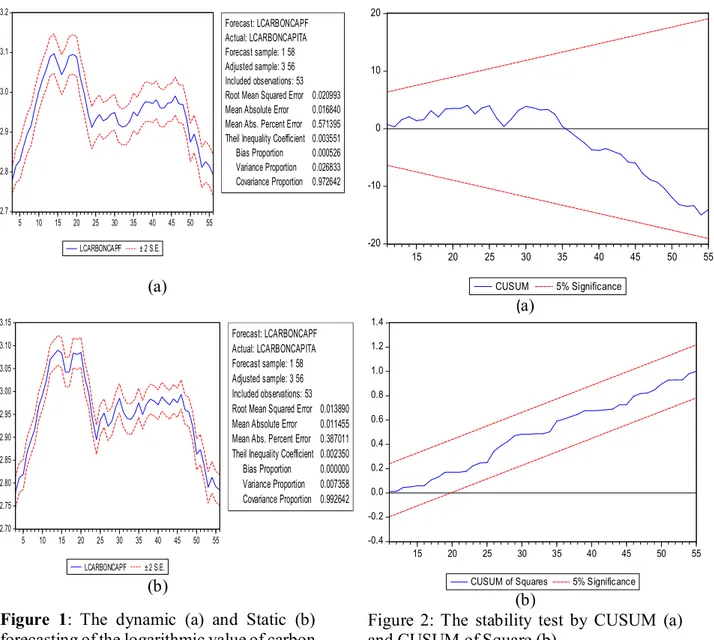
In validating the evidence of cointegration earlier discussed above, the statistical evidence of the bound testing (see Table 3) implies that the evidence of cointegration is significant (F-statistics = 5.977 > I (0) and I (1) critical values), thus valid. This is in addition to the statistical significant result of the Wald test (short-run estimate) as subsequently implied in Table 3. Importantly, further diagnostic test reveal that there is no serial correlation and heteroskedasticity as implied by the Breusch-Godfrey Serial Correlation LM and the Breusch-Pagan-Godfrey heteroskedasticity tests respectively in Table 3. Also, the variables are normally distributed, given the failure to reject the Jarque-Bera statistics (1.067), while they are also positively skewed (0.242). Illustratively, the forecasting of the carbone missions per capita is illustrated in Figure 1 while the stability of the estimation is further affirmed by the Cumulative sum (CUSUM) (a) and CUSUM square test (b) in Figure 2.
2.7 2.8 2.9 3.0 3.1 3.2 5 10 15 20 25 30 35 40 45 50 55 LCARBONCAPF ± 2 S.E. Forecast: LCARBONCAPF Actual: LCARBONCAPITA Forecast sample: 1 58 Adjusted sample: 3 56 Included observations: 53 Root Mean Squared Error 0.020993 Mean Absolute Error 0.016840 Mean Abs. Percent Error 0.571395 Theil Inequality Coefficient 0.003551 Bias Proportion 0.000526 Variance Proportion 0.026833 Covariance Proportion 0.972642 (a) 2.70 2.75 2.80 2.85 2.90 2.95 3.00 3.05 3.10 3.15 5 10 15 20 25 30 35 40 45 50 55 LCARBONCAPF ± 2 S.E. Forecast: LCARBONCAPF Actual: LCARBONCAPITA Forecast sample: 1 58 Adjusted sample: 3 56 Included observations: 53 Root Mean Squared Error 0.013890 Mean Absolute Error 0.011455 Mean Abs. Percent Error 0.387011 Theil Inequality Coefficient 0.002350 Bias Proportion 0.000000 Variance Proportion 0.007358 Covariance Proportion 0.992642
(b)
Figure 1: The dynamic (a) and Static (b) forecasting of the logarithmic value of carbon emissions per capita.
-20 -10 0 10 20 15 20 25 30 35 40 45 50 55 CUSUM 5% Significance (a) -0.4 -0.2 0.0 0.2 0.4 0.6 0.8 1.0 1.2 1.4 15 20 25 30 35 40 45 50 55 CUSUM of Squares 5% Significance
(b)
Figure 2: The stability test by CUSUM (a) and CUSUM of Square (b).
5. Conclusion and Policy Pathway
The growing concern of global warming arising from the adverse weather variation and increasing push for economic dominance among the advanced nations especially the United States accounts for the vast interest in environmental-linked studies. On this note, the current study mainly examined the effect of the degree days (the cooling and heating degree days) and the ecological
footprint accounting of the United States on environmental degradation. While the study is important for the United States because of the vast deficit of ecological footprint of the country (Global Footprint Network, 2019), the United States is equally known to experience significant weather variation in the last decades. Therefore, the current study found that both the cooling and heating degree-days adversely affect environmental quality in the short-run and long-run. Although the long-run impacts are enormous, statistical evidence indicates that the impacts are not significant. However, the impact of the increasing demand of the country’s ecological footprint on environmental degradation is also reportedly positive and significant. This further informs that there is a significant and adverse environmental hazard associated with the deficit accounting of the United States’ ecological footprint. Moreover, the environmental impact of income growth as observed in the result for the United States is expected. The result posits that income growth in the United States especially in the long-run would not improve the environmental quality.
Considering the result-yielding effort of the United States Climate Alliance and other climate-oriented policies, the push for more investment in cleaner and energy efficiency, and climate resilience has reportedly accounted for the reduction of Greenhouse gas between 2005 and 2016 by about 14% (United States Climate Alliance, 2019). In the light of this positive climate and environmental friendlier policies, there is need for stronger weather-oriented policies such that directly or indirectly addresses the adverse effect of the extreme weather conditions (the cooling and heating degree days) across the country. On the other hand, the government and other stakeholders should further encourage strategic plans especially toward the recovery of the ecological footprint accounting across the country. While encouraging policies that are potentially aimed at ecosystem recovery, the government at the central and state levels should further adopt
sustainable and greener economy policies in order to further mitigate the adverse effect of the country’s income growth.
Reference
Adedoyin, F. F., Gumede, M. I., Bekun, F. V., Etokakpan, M. U., & Balsalobre-lorente, D. (2020). Modelling coal rent, economic growth and CO2 emissions: Does regulatory quality matter in BRICS economies? Science of the Total Environment, 710, 136284.
Alola, A. A. (2019). The trilemma of trade, monetary and immigration policies in the United States: Accounting for environmental sustainability. Science of The Total Environment, 658, 260-267.
Alola, A. A. (2019). Carbon emissions and the trilemma of trade policy, migration policy and health care in the US. Carbon Management, 10(2), 209-218.
Alola, A. A., & Alola, U. V. (2018). Agricultural land usage and tourism impact on renewable energy consumption among Coastline Mediterranean Countries. Energy & Environment, 29(8), 1438-1454.
Alola, A. A., Arikewuyo, A. O., Ozad, B., Alola, U. V., & Arikewuyo, H. O. (2020c). A drain or drench on biocapacity? Environmental account of fertility, marriage, and ICT in the USA and Canada. Environmental Science and Pollution Research, 27(4), 4032-4043.
Alola, A. A., Bekun, F. V., & Sarkodie, S. A. (2019). Dynamic impact of trade policy, economic growth, fertility rate, renewable and non-renewable energy consumption on ecological footprint in Europe. Science of The Total Environment, 685, 702-709.
Alola, A. A., & Kirikkaleli, D. (2019). The nexus of environmental quality with renewable consumption, immigration, and healthcare in the US: wavelet and gradual-shift causality approaches. Environmental Science and Pollution Research, 26(34), 35208-35217. Alola, A. A., Saint Akadiri, S., Akadiri, A. C., Alola, U. V., & Fatigun, A. S. (2019a). Cooling and
heating degree days in the US: The role of macroeconomic variables and its impact on environmental sustainability. Science of The Total Environment, 695, 133832.
Alola, A. A., Yalçiner, K., & Alola, U. V. (2019). Renewables, food (in) security, and inflation regimes in the coastline Mediterranean countries (CMCs): the environmental pros and cons. Environmental Science and Pollution Research, 1-11.
Alola, A. A., Yalçiner, K., Alola, U. V., & Saint Akadiri, S. (2019b). The role of renewable energy, immigration and real income in environmental sustainability target. Evidence from Europe largest states. Science of The Total Environment, 674, 307-315.
Apergis, N., & Payne, J. E. (2009). CO2 emissions, energy usage, and output in Central America. Energy Policy, 37(8), 3282-3286.
Apergis, N., & Ozturk, I. (2015). Testing environmental Kuznets curve hypothesis in Asian countries. Ecological Indicators, 52, 16-22.
Bekun, F. V., Alola, A. A., & Sarkodie, S. A. (2019). Toward a sustainable environment: Nexus between CO2 emissions, resource rent, renewable and nonrenewable energy in 16-EU countries. Science of the Total Environment, 657, 1023-1029.
Bekun, F. V., Emir, F., & Sarkodie, S. A. (2019). Another look at the relationship between energy consumption, carbon dioxide emissions, and economic growth in South Africa. Science of
Ehrlich, P. R., & Holdren, J. P. (1971). Impact of population growth. Science, 171(3977), 1212-1217.
Dickey, D. A., & Fuller, W. A. (1981). Likelihood ratio statistics for autoregressive time series with a unit root. Econometrica: journal of the Econometric Society, 1057-1072.
Dietz, T., & Rosa, E. A. (1997). Effects of population and affluence on CO2 emissions. Proceedings of the National Academy of Sciences, 94(1), 175-179.
Dietz, T., & Rosa, E. A. (1994). Rethinking the environmental impacts of population, affluence and technology. Human ecology review, 1(2), 277-300.
Dogan, E., Seker, F., & Bulbul, S. (2017). Investigating the impacts of energy consumption, real GDP, tourism and trade on CO2 emissions by accounting for cross-sectional dependence: A panel study of OECD countries. Current Issues in Tourism, 20(16), 1701-1719.
Global Footprint Network (2019). Ecological Footprint. https://www.footprintnetwork.org/our-work/ecological-footprint/. (Accessed 2 January 2020).
Ike, G. N., Usman, O., Alola, A. A., & Sarkodie, S. A. (2020). Environmental quality effects of income, energy prices and trade: The role of renewable energy consumption in G-7 countries. Science of The Total Environment, 137813.
Isaac, M., & Van Vuuren, D. P. (2009). Modeling global residential sector energy demand for heating and air conditioning in the context of climate change. Energy policy, 37(2), 507-521.
Işık, C., Ongan, S., & Özdemir, D. (2019). Testing the EKC hypothesis for ten US states: an application of heterogeneous panel estimation method. Environmental Science and
Kwiatkowski, D., Phillips, P. C., Schmidt, P., & Shin, Y. (1992). Testing the null hypothesis of stationarity against the alternative of a unit root: How sure are we that economic time series have a unit root? Journal of econometrics, 54(1-3), 159-178.
Li, M., Cao, J., Xiong, M., Li, J., Feng, X., & Meng, F. (2018). Different responses of cooling energy consumption in office buildings to climatic change in major climate zones of China. Energy and Buildings, 173, 38-44.
Moustris, K. P., Nastos, P. T., Bartzokas, A., Larissi, I. K., Zacharia, P. T., & Paliatsos, A. G. (2015). Energy consumption based on heating/cooling degree days within the urban environment of Athens, Greece. Theoretical and Applied Climatology, 122(3-4), 517-529. Mutlu Ozturk, H., Dombayci, O. A., & Caliskan, H. (2019). Life-Cycle Cost, Cooling Degree Day, and Carbon Dioxide Emission Assessments of Insulation of Refrigerated Warehouses Industry in Turkey. Journal of Environmental Engineering, 145(10), 04019062.
Nathaniel, S. P., & Iheonu, C. O. (2019). Carbon dioxide abatement in Africa: The role of renewable and non-renewable energy consumption. Science of the Total Environment, 679, 337-345.
Nathaniel, S., Anyanwu, O., & Shah, M. (2020). Renewable energy, urbanization, and ecological footprint in the Middle East and North Africa region. Environmental Science and Pollution
Research, 1-13.
National Climatic Data Center (2019) What are heating and cooling degree days? National Weather Service. https//www.ncdc.noaa.gov.
Ozturk, I., & Acaravci, A. (2010). CO2 emissions, energy consumption and economic growth in Turkey. Renewable and Sustainable Energy Reviews, 14(9), 3220-3225.
Ozturk, I., Al-Mulali, U., & Solarin, S. A. (2019). The control of corruption and energy efficiency relationship: an empirical note. Environmental Science and Pollution Research, 26(17), 17277-17283.
Pesaran, M. H., Shin, Y., & Smith, R. J. (2001). Bounds testing approaches to the analysis of level relationships. Journal of applied econometrics, 16(3), 289-326.
Saint Akadiri, S., & Alola, A. A. (2020). The role of partisan conflict in environmental sustainability targets of the United States. Environmental Science and Pollution Research, 1-10.
Saint Akadiri, S., Alola, A. A., & Akadiri, A. C. (2019). The role of globalization, real income, tourism in environmental sustainability target. Evidence from Turkey. Science of the total
environment, 687, 423-432.
Saint Akadiri, S., Bekun, F. V., & Sarkodie, S. A. (2019). Contemporaneous interaction between energy consumption, economic growth and environmental sustainability in South Africa: What drives what?. Science of the total environment, 686, 468-475.
Saint Akadiri, S., Alola, A. A., Akadiri, A. C., & Alola, U. V. (2019a). Renewable energy consumption in EU-28 countries: policy toward pollution mitigation and economic sustainability. Energy Policy, 132, 803-810.
Saint Akadiri, S., Alola, A. A., Olasehinde-Williams, G., & Etokakpan, M. U. (2019b). The role of electricity consumption, globalization and economic growth in carbon dioxide emissions and its implications for environmental sustainability targets. Science of The Total
Environment, 134653.
Shahbaz, M., Solarin, S. A., Hammoudeh, S., & Shahzad, S. J. H. (2017). Bounds testing approach to analyzing the environment Kuznets curve hypothesis with structural beaks: The role of biomass energy consumption in the United States. Energy Economics, 68, 548-565.
Solarin, S. A., & Bello, M. O. (2018). Persistence of policy shocks to an environmental degradation index: the case of ecological footprint in 128 developed and developing countries. Ecological indicators, 89, 35-44.
Solarin, S. A., & Bello, M. O. (2020). Energy innovations and environmental sustainability in the US: The roles of immigration and economic expansion using a maximum likelihood method. Science of The Total Environment, 712, 135594.
United States Climate Alliance (2019). http://www.usclimatealliance.org/state-climate-energy-policies/ (Accessed 02 January 2020).
Udemba, E. N. (2019). Triangular nexus between foreign direct investment, international tourism, and energy consumption in the Chinese economy: accounting for environmental quality. Environmental Science and Pollution Research, 26(24), 24819-24830.
Udemba, E. N., Güngör, H., & Bekun, F. V. (2019). Environmental implication of offshore economic activities in Indonesia: a dual analyses of cointegration and causality. Environmental Science and Pollution Research, 26(31), 32460-32475.
Udi, J., Bekun, F. V., & Adedoyin, F. F. (2020). Modeling the nexus between coal consumption, FDI inflow and economic expansion: does industrialization matter in South Africa? Environmental Science and Pollution Research, 1-12.
Usman, O., Iortile, I. B., & Ike, G. N. (2020). Enhancing sustainable electricity consumption in a large ecological reserve–based country: the role of democracy, ecological footprint, economic growth, and globalisation in Brazil. Environmental Science and Pollution
Research, 1-14.
Usman, O., Olanipekun, I. O., Iorember, P. T., & Abu-Goodman, M. (2020). Modelling environmental degradation in South Africa: the effects of energy consumption, democracy,
and globalization using innovation accounting tests. Environmental Science and Pollution
Research, 1-16.
Wackernagel, M., Lin, D., Evans, M., Hanscom, L., & Raven, P. (2019). Defying the Footprint Oracle: Implications of Country Resource Trends. Sustainability, 11(7), 2164.