NUMBER : 1
Received Date : 04.09.2002
GENERALIZED MODELING PRINCIPLES OF A NONLINEAR
SYSTEM WITH A DYNAMIC FUZZY NETWORK
A.Ferit KONAR
1Yusuf OYSAL
21Department of Computer Eng. Doğuş University, İstanbul, TURKEY 2Department of Computer Eng. Anadolu University, Eskişehir, TURKEY
ABSTRACT
Generalized modeling principles of a nonlinear system with a dynamic fuzzy network (DFN)- a network with unconstrained connectivity and with dynamic fuzzy processing units called ‘feurons’, have been given. DFN model has been trained both in open loop and closed loop forms to satisfy these principles. Several system trajectories with a PRBS input have been used for open loop training. DFN model obtained from open loop training was used in a closed loop training with an extended Kalman filter (EKF) in an observer design. For gradient computations adjoint sensitivity method has been used.
Keywords: Intelligent Systems, Fuzzy Logic, Neural Networks, Generalized Modeling
I. INTRODUCTION
The application of fuzzy logic technology to modeling and control of dynamical systems has been constrained by the non-dynamical nature of popular fuzzy system architectures. Many of the difficulties that ensue- large rule bases (i.e., curse of dimensionality), long training times, the need to determine buffer lengths- can be overcome with dynamic fuzzy network (DFN)- network realizations that contain unconstrained connectivity and with dynamic fuzzy processing units called “feurons” and may also allow for the incorporation of both heuristics and deep knowledge to exploit the best characteristics of each [12, 21].
The two major complications introduced during the modeling of a nonlinear dynamical system with a DFN are: which principles should be considered to obtain the accurate “model equivalence” of a known model of a nonlinear dynamical system? Moreover, how can we train
a DFN for the best convergence? For the first one, the generalized modeling principles have been defined in this study. In algebraic fuzzy systems parameter tuning is relatively simple because the gradients of model error with respect to the parameters are easy to compute [20]. In dynamic fuzzy networks, gradient computation is more involved. Approaches for gradient computation for dynamic systems have been developed in systems and control theories [2, 21], and have been successfully used in identification and control applications [9, 10]. In section 2, we define the generalized modeling principles. In section 3, we introduce the standard fuzzy system. In section 4, we present a model for dynamic fuzzy network (DFN). In sections, we have discussed the employment of approximate second order gradient-based approaches to determine appropriate values for the dynamic fuzzy network parameters for the desired trajectory tracking and modeling.
Simulation examples of phase portrait modeling of a tunnel diode circuit by a DFN and open loop and closed loop modeling of a CSTR system by a DFN are illustrated in section 6.
2. GENERALIZED MODELING
PRINCIPLES
To make an effective control system design, there should be a model that accurately represents the real nonlinear dynamical plant. Theoretical models are obtained in general, by four steps [3, 15]. These are 1) problem definition, 2) model formulation by using the first principles, 3) parameter estimation and 4) model validation.
It is asserted that there exists a DFN which can represent all the behaviors of a given dynamical plant. This assertion is based on the experiments done on a mathematical models that accurately represent the physical plant (i.e., reference model). We can develop an equivalent DFN which captures all the qualitative behaviors of this physical plant. In this study these experiments classified into two categories: i) open loop/closed loop validations, ii) local and global validations.
There are some works in the literature for open loop and closed loop verification of a model. Gevers (1999), developed the model error estimation method of Ljung (1987) for the closed loop validation. Some examples of open loop validation can be found in Aguirre’s studies [1].
3. STANDARD FUZZY SYSTEM
An important contribution of fuzzy systems theory is that it provides a systematic procedure for transforming a knowledge base into a nonlinear mapping [20]. Figure 3.1 shows the basic configuration of a fuzzy system.
Figure 3.1 Basic configuration of fuzzy systems
We call the fuzzy systems with product inference engine, singleton fuzzifier, center average defuzzifier, and Gaussian membership functions as “standard fuzzy systems” [20]. Nonlinear mapping of a standard fuzzy system is in the following form:
∑∏
∑ ∏
= = σ − = = σ −−
−
=
r 1 i n 1 j 2 ij ij c j x 2 1 r 1 i n 1 j 2 ij ij c j x 2 1 i)
)
(
exp(
)
)
(
exp(
y
)
x
(
f
(3.1)where r is the number of rules, cij and σij are
center and spread parameters of the ith rule’s jth
input variable’s of the Gaussian membership function respectively. yi, is the output center
parameter of the ith rule. Figure 3.2 shows the
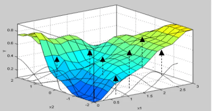
inference mechanism of a standard fuzzy system with two input variables that uses expert knowledge base.
Figure 3.2 The inference mechanism of a standard fuzzy system with two input variables.
(Peaks show some expert knowledge)
4. THE DYNAMIC FUZZY
NETWORK (DFN) MODEL
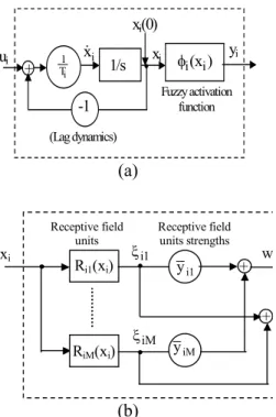
By a dynamic fuzzy network, we mean a network with unconstrained connectivity and with dynamic elements in its fuzzy processing units [13, 17]. The processing unit is called the feuron, representing a single dynamic fuzzy neuron. Figure 4.1 shows a DFN with two feurons.
Basically the feuron model represents the biological neuron that fires when its inputs are significantly excited. This firing is through a lag dynamics (i.e., Hopfield dynamics). The manner in which the feuron fires is defined by the fuzzy
activation function φ. The feuron's activation model also represents a standard fuzzy system that described before.
F1
F2
u y
Figure 4.1 Dynamic Fuzzy Network (DFN) with two feurons 1/s 1 Ti + φi(xi) -1 xi &xi yi xi(0) Fuzzy activation function (Lag dynamics) ui (a) Ri1(xi) RiM(xi) yi1 yiM + + xi w Receptive field units Receptive field units strengths 1 i ξ iM ξ (b)
Figure 4.2 Block diagram of the feuron (a) A single feuron model, (b) Feuron’s activation model, yi= φ(xi).
Since the feuron's activation model has a single input, (i.e., the scalar state of the feuron) the product inference output becomes the membership functions itself. The activation function of the ith feuron can be expressed as:
( )
( )
∑
∑
∑
∑
= σ − = σ − = = − − = µ µ = φ i R 1 k 2 ik ik c i x 2 1 i R 1 k 2 ik ik c i x 2 1 ik i R 1 k k i i k i R 1 k ik i i exp exp b ) x ( ) x ( b ) x ( (4.1) The boundary membership functions of the feuron may be represented by hard constraints in the form of:iU i i i R iL i i 1
(
x
)
=
1
,
if
x
≤
x
and
µ
(
x
)
=
1
,
if
x
≥
x
µ
(4.2) where xiL and xiU are the lower and upper limitsof the state values of the ith feuron respectively.
The general computational model that we have used for DFN is summarized in the following equations:
∑
==
n 1 j j mj mq
y
z
(4.3))
,
x
(
y
i=
φ
i iπ
i (4.4) 0 i i i l 1 j j ij n 1 j j ij i i ix
x
w
y
p
u
+
r
,
x
(
0
)
x
T
=
−
+
∑
+
∑
=
= =&
(4.5) where w, p, q, r are the interconnection parameters of the DFN, T is the time constants and π is the parameter sets (centers c, spreads σ, output centers b) corresponding to fuzzy SISO activation functions of the feurons. This model has some similarities with models encountered in the literature [6, 16].5. PERFORMANCE INDEX
MINIMIZATION IN DFN
In order to obtain DFN model of a process we associate a performance index given by
∫
−
−
=
tf 0 d T d(
t
)]
[
z
(
t
)
z
(
t
)]
dt
z
)
t
(
z
[
2
1
J
(5.1)where zd(t) and z(t) are actual and modeled
process responses respectively. Tuning dynamic fuzzy networks to mimic a given set of trajectories is equivalent to determining (i.e., learning) DFN parameters so that the performance index is minimized. This is a dynamic nonlinear optimization problem. We require the computation of gradients or sensitivities of the performance index with respect to the various interconnection parameters of the DFN and internal parameters of the feurons. They are respectively:
]
b
J
,
J
,
c
J
,
T
J
[
and
]
r
J
,
q
J
,
p
J
,
w
J
[
∂
∂
∂σ
∂
∂
∂
∂
∂
∂
∂
∂
∂
∂
∂
∂
∂
(5.2) We have used “Adjoint’’ method for sensitivity computation [10]. The computation formulas have been found in [15]. We used first and approximate second order gradient-based methods including Broyden-Fletcher-Golfarb-Shanno (BFGS) algorithm to update the parameters of the dynamic fuzzy networks yielding faster rate of convergence [4, 19].6. GENERALIZED MODELING
SIMULATION EXAMPLES
For obtaining the equivalent DFN models due to generalized modeling principles, first of all it is useful to show the efficiency of a DFN in global modeling. Our first set of experiments have used the data of a tunnel diode circuit with two state variables for phase portrait modeling by a DFN with two feurons.
6.1 Phase Portrait Modeling of a
Tunnel Diode Circuit
The state-space model of a tunnel diode circuit [7] is given by
[
1 2 1h
(
x
)
x
C
1
x
&
=
−
+
]
(6.1)[
x
Rx
u
L
1
x
&
2=
−
1−
2+
]
(6.2) where h(x) is a fifth degree polynomial representing the tunnel diode charecteristics and given by
h(x)=17.76x-103.79x2+229.62x3-226.31x4+83.72x5 (6.3)
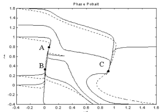
and the other circuit parameters are given as u=1.2 V, R=1.5 kΩ, C=2 pF, L=5 µH (6.4) The tunnel diode circuit system was simulated for several initial conditions to the three equilibrium points A=(0.285,0.61), B=(0.063,0.758), and C=(0.884,0.21) with an integration time step of 0.01 second. These trajectories were taken as the desired trajectories for a DFN to capture. At the beginning, each trajectory segment was used for training. Subsequently, combinations of the segments
were used for fine-tuning based on randomly generated initial conditions. Figure 6.1 shows the resulting phase portraits of the tunnel diode circuit system and the DFN model. The final phase portrait model response was visually indistinguishable in some of the trajectory segments.
Dynamic fuzzy network parameters obtained were: = = = − = 2 . 1 0 r , 1 1 q , 0 0 p , 20.2944 28.8822 39.2152 7369 . 57 w 3875 . 7 4384 . 7 0564 . 24 4820 . 15 1482 . 3 1823 . 65 1915 . 16 9189 . 23 1549 . 1 3997 . 15 b , 4307 . 80 4181 . 151 4817 . 40 7712 . 201 8831 . 57 0666 . 1 5575 . 64 2121 . 0 4998 . 0 3802 . 31 , 3446 . 108 6273 . 225 5070 . 174 3668 . 254 0508 . 23 9055 . 4 6096 . 10 7567 . 0 6517 . 5 4851 . 6 c , 5 0 0 2 T − − − − − − − = = Σ − − − − − − = =
Figure 6.1 The phase portrait of the DFN (dashed curve). The solid curve is the Tunnel Diode circuit phase portrait.
6.2 Equivalent DFN Modeling of a
Nonlinear Continuously Stirred Tank
Reactor
Generalized modeling principles given in section 2 have been examined for obtaining a DFN model equivalent of a nonlinear continuously stirred tank reactor (CSTR) system with relevant equations given below [18]:
γ + − + − = 1 x2 2 x 1 1 1 x Da(1 x )e dt dx (6.5) (6.6) where x1, x2 represent dimensionless reactant
conversion and temperature, Da is the Damköhler number and the variables d, u are dimensionless deviation variables for the feed temperature disturbance and control (jacket temperature) respectively. In the simulations the parameters were taken as Da= 0.135, B=11, β=1.5 and γ =20.
For the equivalent DFN modeling of a CSTR, these experiments have been done:
1) Open loop:
• Zero-input response of the equivalent models,
• Zero-state response of the equivalent models,
• Various input and various state responses of the equivalent models,
2) Closed loop:
• The design of Extended Kalman Filter with equivalent models,
6.2.1 Open Loop Experiments
To obtain an equivalent DFN model, we have used data generated from a simplified nonlinear CSTR model as the target model. Performance index has been chosen as:
∫
−
+
−
=
tf 0 2 2 2 2 1 1(
xd
x
)
dt
2
1
)
x
xd
(
2
1
J
x
ˆ
kk=
xˆ
k k−1+
Kˆ
k(
z
k−
zˆ
kk−1)
(6.7)where x1 are x2 normalized CSTR concentration
and temperatures respectively. xd1 and xd2 are
state variables (feuron variables) of DFN. CSTR initial states have been taken as zero. A PRBS has been applied to this system. Approximately in 83 iterations the equivalent DFN model responses converges to the CSTR responses. Figure 6.2 illustrates the change of DFN state responses for some iterations.
To examine the validity of obtained equivalent DFN model, we have also examined the
steady-state responses and the eigenvalues of the equivalent systems. Figure 6.3 shows that both system responds exactly the same.
6.2.2 Closed Loop Experiments
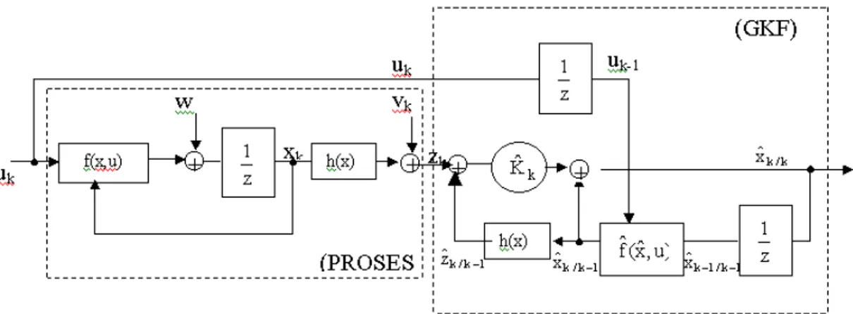
For validation of the equivalent DFN model obtained from the open loop experiments, it is necessary to examine some of the closed loop responses of the equivalent models. For this aim equivalent DFN model obtained from open loop training was used in an extended Kalman filter (EKF) in an observer design.
EKF is based on the linearization of a nonlinear system around an operating point or a trajectory and application of linear optimal state estimation to the obtained system [2, 14]. Figure 6.4 shows the block diagram of linearized EKF. The k indices is a discrete time indices. k/k-1 indices represents the k indices variable that uses (k-1)th
indices and previous indices values. Process model can be written as:
k k k 1 k
f
(
x
,
u
)
w
x
+=
+
k k kh
(
x
)
v
z
,+
=
(6.8) where wk and vk are random variables with Q andR covariance and zero mean respectively. EKF equations can be summarized as: 1) One-step ahead prediction equations:
)
u
,
xˆ
(
fˆ
xˆ
kk−1=
k−1k−1 k−1 ,zˆ
kk−1=
h
(
xˆ
kk−1)
2) Correction equations: 3) Covariance propagation 1 k T 1 k 1 k 1 k 1 k 1 k kF
P
F
Q
P
−=
− − − −+
− 4) Covariance correction: 1 k k k k k k(
I
Kˆ
H
)
P
P
=
−
− 5)Filter gain: 1 k T k 1 k k k T k 1 k k kP
H
(
H
P
H
R
)
Kˆ
=
− −+
−The gradients with respect to system state variables are:
1 k 1 k xˆ k 1 k 1 k xˆ 1 k
x
h
H
,
x
fˆ
F
− − − − −=
∂
∂
=
∂
∂
(6.9) For one step ahead prediction equationsxˆ
0−1 and for covariance propagation P0/-1 valuesshould be selected first.
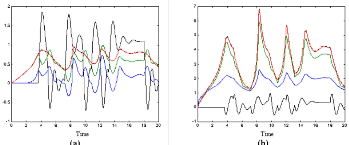
To test the generalized modeling principles, the equivalent DFN model obtained from the open loop training has been used in linearized EKF to estimate the CSTR model states. Figure 6.5 shows CSTR response with covariance process noise and zero initial conditions to zero input. When EKF has been applied for state estimation with the initial parameters chosen as:
it can be seen that estimation was successful (Figure 6.5).
Closed loop experiments can be expanded for various closed loop control appications from PID controller to fuzzy controllers, etc. In [17] the results of the closed loop PID control systems for a CSTR and its equivalent DFN models have been shown. It has been seen that equivalent models exactly gave the same responses to the PID controller under various disturbance effects.
Figure 6.2 DFN (model) response (solid curves at start) (a) concentration (b) temperature. The dashed and near solid curves are Process and DFN (converged model) responses, respectively.
Figure 6.3 The solid and near dashed curves are Process and DFN responses to change in feed temperature respectively (a) steady-state responses, (b) the change of eigenvalues.
Figure 6.4 Block diagram of linearized Extended Kalman Filter (EKF)
Figure 6.5 (a) CSTR responses with white process and measurement noise, (b) CSTR responses without noise (solid curve) and EKF with DFN estimations (dashed curves)
7. CONCLUSIONS
This work is the result of our ongoing research on Intelligent Systems. It is a companion paper to earlier works given in [8, 10, 12] on Dynamic Neural Networks. The work reported here has concentrated on laying the theoretical and analytic foundations for training of Dynamic Fuzzy Network DFN. They are to be used in real-time applications with process modeling and advanced control.
For modeling with DFN, “extended equivalence conditions” have been defined. DFN model has been trained both in open loop and closed loop forms to satisfy these equivalence conditions.
Several system trajectories with a PRBS input have been used for open loop training. DFN model obtained from open loop training was used in an extended Kalman filter (EKF) in an observer design for a nonlinear system. It has been shown by simulations that DFN system models satisfy all extended equivalence conditions.
REFERENCES
[1] Aguirre L. A., “Open-loop Model Matching in Frequency Domain”, Electronics Letters, vol. 28, pp 484-485, 1992
[2] Bryson A. E., and Ho Y. C., Applied Optimal
Control. Hemisphere, 1975.
[3] Burton T. D., Introduction to Dynamic
Systems Analysis, McGraw-Hill, Inc., 1994
[4] Edgar T. F., and Himmelblau D. H.,
Optimization of Chemical Processes.
McGraw-Hill, 1988.
[5] Gevers M., Codrons B., De Bruyne F., “Model Validation in Closed-loop”, Proc. Of the 1999 American Control Conference, 326-330, San Diego, CA, USA,1999
[6] Jordan M. I., “Attractor dynamics and parallelism in connectionist sequential machine.’’ Proc. of the Eighth Annual
Conference of Cognitive Science Society.
Hillsdale, N.J.: Lawrence Erlbaum Associates, 1986.
[7] Khalil H. K., Nonlinear Systems, Prentice-Hall, NJ, 1996
[8] Konar A. F., et al, XIMKON: an expert
simulation and control program. In Artificial
Intelligence and Process Engineering. New York: Academic Press, 1990.
[9] Konar A. F., and Samad T., “Hybrid Neural Network/ Algorithmic System Identification.’’
Technical Report SSDC-91-I4051-1, Honeywell SSDC, 3660 Technology Drive, Minneapolis,
MN 55418, 1991.
[10] Konar A. F., and Samad T., “Dynamic Neural Networks.’’ Technical report SSDC-92-I
4142-2, Honeywell Technology Center, 3660
Technology Drive, Minneapolis, MN 55418, 1992.
[11] Konar A. F., and Samad T., “Philosophical Aspects of Intelligent Control,” IEEE Int. Symp.
On Intelligent Control (ISIC’97), İstanbul 1997
[12] Konar A. F., Becerikli Y. and Samad T., “Trajectory Tracking With Dynamic Neural Networks,” IEEE Int. Symp. On Intelligent
Control (ISIC’97), İstanbul 1997
[13] Konar A. F., Oysal Y., Becerikli Y., Samad T., “Dynamic Fuzzy Networks for Real-Time Applications”, Türkiye Artificial Intelligence &
Neural Network Symposium, TAINN'99, Bogaziçi
University, March 1999
[14] Lewis F. L., Optimal Estimation, John Wiley and Sons, New York, 1986
[15] Ljung L., System Identification Theory for
the User, Prentice-Hall, N. J., USA, 1987
[16] Morris A. J., “On artificial neural networks in process engineering.’’ IEE Proc. Pt. D.
Control Theory and Applications, 1992.
[17] Oysal Y., Fero Modelleme ve Optimal Bulanık Kontrol, Doktora Tezi, Sakarya
Üniversitesi, Fen Bilimleri Enstitüsü, Mart 2002
[18] Ray. W. H., “New Approaches to the Dynamics of Nonlinear Systems with Implications for Process and Control Design.”
Chemical Process Control, Edgar Seaburg
Editions, 2:119, 1981
[19] Shanno D. F., “ Conditioning of Quasi-Newton for function minimization.”, Math.
Comp.,24:647-656, 1970.
[20] Wang L. X., A Course in Fuzzy Systems and
Control, Prentice-Hall International, Upper
Saddle River, New Jersey, 1997.
[21] Zadeh L. A.,. and Desoer C. A., Linear
System Theory, McGraw-Hill Book Company,
NewYork, 1963.
A. Ferit Konar received the B.S.E.E. degree from Yıldız Technical University, Istanbul, Turkey in 1952, M.S.E.E. and M.S. MATH. degrees from the University of Michigan, AnnArbor, MICH. USA, in 1957 and 1961 respectively and the Ph.D. degree in Control Science, from the University of Minnesota, Twin Cities, MN; USA in 1969. Currently he is a Professor of Computer Engineering, in Doğuş University, Istanbul, TURKEY. His current research interests are, System Theories, Neuro, Fuzzy Optimal Control, and Large-scale Software Systems development. He is the architect of the XIMKON-Expert Simulation and Control Software System widely used in the Aerospace and Defense Industries in USA and holds three US patents in Neural Networks. Dr. Konar has been a Senior Member of the IEEE Control Engineering Society since 1969 and a Member of the Sigma Xi Honor Society since 1957.
Yusuf Oysal was born in 1970 in Eskişehir. He received the B.S. degree in electrical and electronic engineering from Middle East Technical University, Ankara. He received the M.S. and Ph.D. degrees in electronic
engineering in 1995 and 2002 from Sakarya University. He is now studying in computer engineering
department of Anadolu University. His current research interests include fuzzy logic, neural networks, optimal control, adaptive control and wavelet transformation.