Multihoist Cyclic Scheduling With
Fixed Processing and Transfer Times
Yun Jiang and Jiyin Liu
Abstract—In this paper, we study the no-wait multihoist cyclic
scheduling problem, in which the processing times in the tanks and the transfer times between tanks are constant parameters, and de-velop a polynomial optimal solution to minimize the production cycle length. We first analyze the problem with a fixed cycle length and identify a group of hoist assignment constraints based on the positions of and the relationships among the part moves in the cycle. We show that the feasibility of the hoist scheduling problem with fixed cycle length is consistent with the feasibility of this group of constraints which can be solved efficiently. We then identify all of the special values of the cycle length at which the feasibility property of the problem may change. Finally, the whole problem is solved optimally by considering the fixed-cycle-length problems at these special values.
Note to Practitioners—Automated electroplating lines are
com-monly used in the production of many products, such as printed-circuit boards. The productivity of these systems depends heavily on effective scheduling of the material handling hoists that move the products between the processing tanks. This paper studies the hoist scheduling problem in systems where the processing times in the tanks and the intertank move times are fixed parameters. An efficient optimal algorithm is developed to solve the problem with any number of hoists. The resulting schedule can be programmed as programmable logic controller codes to directly control the hoist operations. The algorithm can also be used to develop heuristic so-lutions for multihoist scheduling in systems where the processing times may vary in given intervals.
Index Terms—Hoist scheduling, multiple hoists, no-wait,
optimization.
I. INTRODUCTION
E
LECTROPLATING is a common process in the produc-tion of many products, such as printed-circuit boards (PCBs). An electroplating system is an automated production line with a series of tanks that contain the required chemical so-lutions. Tanks are also called processing stations. Fig. 1 shows a sample electroplating line. The parts to be processed must visit a given sequence of tanks according to the technological requirements. The required processing time in a tank may be a fixed parameter or a flexible parameter within given limits (the limits define a feasible window for the processing time). Hoists mounted on a common track are used to move the parts Manuscript received September 30, 2005; revised January 16, 2006. This paper was recommended for publication by Associate Editor K. Saitou and Editor N. Viswanadham upon evaluation of the reviewers’ comments.Y. Jiang is with Bilkent University, Ankara 06800, Turkey (e-mail: [email protected]).
J. Liu is with Loughborough University, Leicestershire LE11 3TU, U.K. (e-mail: [email protected]).
Digital Object Identifier 10.1109/TASE.2006.884057
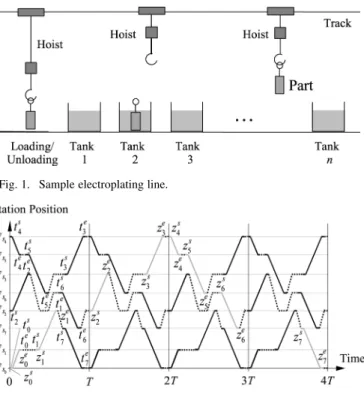
Fig. 1. Sample electroplating line.
Fig. 2. Sample of a time-way diagram.
between the tanks. Effective operations of the hoists are vital to achieve high productivity of the line.
An electroplating line normally produces identical parts cyclically. In each cycle, one part enters the line and another leaves the line after completing all of the required processing steps. Without loss of generality, we take the time point at which a part starts moving to the first tank as the starting point of a cycle. The duration of a cycle is called the cycle length. Since there can be a number of parts being processed at the same time in different tanks of the system, each part can stay in the system for several cycles. Each hoist repeats a sequence of part moves in every cycle. The cyclic production can be illustrated by a “time-way diagram” such as the one in Fig. 2. A time-way diagram is a special type of Gantt Chart emphasizing the hoist movements. The horizontal axis represents time and the vertical axis represents positions along the electroplating line. We use horizontal thin gray lines to show the station positions and use solid lines to indicate the part moves between stations, where a horizontal segment indicates either lifting up or dropping off of a part at a station and an inclined segment indicates the travel between two stations. The processing time of a part at a station is the duration between the ending point of the move to this station and the starting point of the move away from the same station. Dotted inclined lines are used to show empty hoist moves while a dotted horizontal line indicates hoist 1545-5955/$25.00 © 2007 IEEE
waiting at a position. All of the loaded and empty moves of a hoist form the route of that hoist. Since the hoists cannot run across each other on the track, the routes of any two hoists will never have intersection in the time-way diagram. The symbols on the diagram in Fig. 2 will be explained and used later.
The hoist scheduling problem is to allocate the hoists to per-form all of the required part moves in a cycle to maximize the production throughput (i.e., minimize the cycle length).
Most previous research on hoist scheduling focuses on the problem that considers only one hoist and that requires the pro-cessing time in each tank to take a value within a given window. Reference [1] proved that such a single-hoist problem was NP complete. To find optimal cyclic hoist schedules, researchers tried integer programming models (e.g., [2], [3], and [4]) and branch-and-bound algorithms (e.g., [5]–[7] and [8]). For the special case where the hoist route (the sequence of the moves) is given, [9] developed a pseudopolynomial algorithm. Reference [10] presented a polynomial search algorithm for the no-wait single-robot scheduling problem in manufacturing cells, which is equivalent to the no-wait single-hoist scheduling problem. The no-wait condition indicates that the part processing times in the tanks and the transfer times between tanks are all fixed and that, upon completion of the processing in a tank, a part needs to be moved immediately to the next tank.
The multihoist problem is more complicated and has received less research. It involves new decisions on hoist assignment and has to avoid hoist crossings and collisions as more than one hoist runs on the same track. Reference [11] provided a re-view of research on a broader problem class of cyclically sched-uling transporters, including hoists, robots, and other vehicles in flowshops. Reference [12] proposed a mathematical model for general periodical scheduling problems and presented some relevant applications. It can be seen from these references that studies on multitransporter problems are limited and most of them do not consider the common-track constraint. Reference [13] considered two hoists in a special system where parts visit the tanks one by one in one direction from the loading sta-tion to the unloading stasta-tion. They partista-tioned the line into two nonoverlapping zones and then assigned one hoist to perform the intertank part moves in each zone. The optimal schedule was then determined by solving the two single-hoist problems alter-nately. Reference [14] studied a multidegree cyclic two-robot scheduling problem in a no-wait flowshop without the common-track constraint. A different problem but related to multihoist cyclic scheduling is to determine the minimum number of hoists for a system. References [15] and [16] proposed heuristics for minimizing the number of hoists in electroplating lines. Ref-erences [17] and [18] studied the problem of minimizing the number of transporters in other systems without the common-track constraint.
For the no-wait two-hoist cyclic scheduling problem with fixed processing and transfer times, [19] developed a polyno-mial solution algorithm that allows any part flow pattern. They identified and searched over the threshold values of the cycle length. The optimal cycle length was then obtained by checking the feasibility of each threshold cycle length. An optimal schedule was constructed by considering many different com-binations in assigning hoists to a pair of moves. The method is
quite efficient for the problem with two hoists. However, such analysis is difficult to be extended to multiple hoists because the hoist-assignment combinations will be too complicated to handle efficiently. To solve the no-wait multihoist problem, new approaches are needed.
In this paper, we study the no-wait multihoist cyclic sched-uling problem with any number of hoists and an arbitrary part flow pattern, and develop a polynomial optimal solution algorithm. We first describe this problem formally, analyze the basic relationships between the cycle length and the timing of the moves in the cycle, and present a lowerbound and an upperbound of the cycle length (Section II). For any fixed cycle length, we identify a group of hoist assignment constraints in Section III. In Section IV, we prove that the feasibility of this constraint group is consistent with the feasibility of the corresponding cycle length. Based on this, the hoist scheduling problem for any given cycle length can be solved using an efficient algorithm. In Section V, a set of special cycle lengths, that may cause feasibility change, is identified. Section VI summarizes all of these developments and presents a com-plete algorithm that searches for the optimal cycle length and constructs an optimal schedule. An example is also given. Section VII concludes the paper.
II. PROBLEMDEFINITION ANDANALYSIS
In a similar way as defining the no-wait two-hoist problem in [19], we formally describe the no-wait multihoist scheduling problem as follows. Consider an electroplating system with sta-tions arranged in a line from left to right: the loading station (station 0), processing stations (stations ), and pos-sibly an unloading station (station ). The position of
sta-tion is , . Some systems do not have
a separate unloading station. In these systems, loading and un-loading are performed at the same station (station 0) and, there-fore, . Each station can process, at the most, one part at a time. There are hoists on the same track over the line for moving parts between stations. The hoists cannot travel across each other. We denote the hoists from left to right as
. The leftmost position that can reach is and the rightmost position that can reach is . The range
covers the positions of all stations. To avoid collision, any two adjacent hoists must maintain at least a safety distance
between them.
The sequence of stations to be visited by each part, also called
part flow pattern, is given as ,
where is the loading station, is the unloading
sta-tion, and , is the station for the th processing
stage of the part. The required processing time at processing
sta-tion is a given parameter , . After processing
at station , the part must be immediately moved to station by a hoist. We denote this move as . The move consists of lifting up the part from station , carrying the part from station to station , and dropping off the part into station . The time needed for the hoist to lift up or drop off a part at a sta-tion is (the developments of this paper can be easily extended to situations where liftup time and dropoff time are different). The traveling speed of a hoist carrying a part is , and the
As described in Section I, the hoist moving in one cycle is exactly the same as those in any other cycle. There is one part entering the system at the beginning of each cycle. For the part entering the system at time 0, the starting time and ending time of move for this part can be calculated from the parameters using the following formulas:
starting points (1)
ending points (2)
For the example shown in Fig. 2, the moves for the part that enters the system at time 0 are drawn in gray solid lines (lighter than the moves of other parts), and the starting and ending points of these moves are marked. In each production cycle, a move
starting from each station , , is performed
exactly once. For a given cycle length , the starting times of all the required moves in a cycle can be calculated from as follows:
(3) For convenience in later discussions, we define the ending time of moves, with respect to , as follows:
(4)
Let , then
(5) (6) The relationships among , , , and can be seen in Fig. 2.
Definition 1: A feasible hoist schedule is a cyclic schedule in
which each part move is assigned to a hoist; between any two part moves assigned to the same hoist, there is enough time for the empty move of the hoist; and the distance between any two hoists is not shorter than at any time.
Definition 2: A cycle length is said to be feasible if a fea-sible cyclic hoist schedule exists with this cycle length.
The no-wait multihoist cyclic scheduling problem can then be defined as to find the shortest feasible cycle length and a corresponding feasible schedule.
Since each station can process, at most, one part at a time, a feasible cycle length cannot be shorter than the processing time of any station plus the time for moving the finished part away from this station and moving a new part into it. The two moves may be performed by different hoists but the hoists have to keep the safety distance. This provides a method to determine a lowerbound of the optimal cycle length. On the other hand, if a feasible solution exists for the problem, the total time spent by a part in the system provides an upperbound of the optimal cycle length. The above discussion is valid for systems with any number of hoists and directly leads to the following result.
Proposition 1: If there is a feasible solution for the no-wait
multihoist scheduling problem, then
is a lowerbound and
is an upperbound for the optimal cycle length.
III. HOIST ASSIGNMENT CONSTRAINTS FOR AFIXEDCYCLELENGTH
For any given cycle length , , the starting and ending times of all moves in a cycle are fixed in the time-way di-agram and can be calculated from (1)–(4). The problem then be-comes verifying the feasibility of the cycle length by searching for a feasible assignment of the moves to the hoists. In this sec-tion, we identify necessary conditions that must be satisfied by a feasible assignment compatible with the value of the cycle length.
We define the following variables for the hoist assignment decisions.
: the hoist number assigned to perform , , in every cycle.
A. Constraints by Positions of Individual Moves
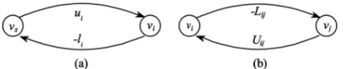
Recall that the hoists run on the same track and are numbered from left to right. If the distance from the position of a tank to the track’s leftmost position is less than the safety distance , then this tank can only be reached by , and any move from or to this tank must be performed by . Similarly, if the distance of a tank to is less than , then the moves involving this tank can only be performed by or . Considering the value range of , , such restrictions can be represented by
Similarly, the track’s rightmost position imposes the fol-lowing constraint:
These constraints set tighter bounds for . Denoting and , we can write them in the following form:
(7) Fig. 3 illustrates these constraints for a move. Note that these constraints are independent of . Therefore, if they are infea-sible, then the hoist scheduling problem is infeasible.
B. Constraints From Hoist Assignment of One Move
Since the hoists cannot be very close to each other, the hoist assignments of a pair of moves are also restricted by the
rela-Fig. 3. Illustration of constraints by the position of an individual move.
tionship of the two moves in time and in position. As prepa-ration for presenting these move–pair relation constraints con-cisely (in Section III-C), we first discuss here the constraints imposed by the hoist assignment of one move on positions of all hoists. Consider a move and an arbitrary point
in the time-way diagram. Suppose is assigned to hoist , then the hoists that can reach the point are restricted by this assignment. We denote a hoist that can reach this point as and identify the constraints that limit the possible values of . The diagram in Fig. 4 illustrates the move and the bounding lines around it. For point being in different areas sep-arated by these lines, the bounds for are different and marked in the diagram. From the diagram, we can see that the format of the constraints may be different when the point is at different positions with respect to move . In the following, we discuss these different situations.
For the case , we denote the position of hoist at time as . Since is performed by , the position of at
time will be . Due to the safe distance between
two adjacent hoists, we have for
(i.e., for is the same as or is a hoist below on
the diagram), and for (i.e., for
is the same as or is a hoist above on the diagram). To
reach the point from , hoist should be able
to arrive at position on or before the time in the maximum empty move speed . Therefore, we have
for for
Considering that and are integers, the first inequality above (for ) can be written as
for
With the condition , this constraint can be satisfied only
when . Reversely, when
(i.e., the point
is above the top upwards-sloped dotted line on the right part of Fig. 4), the condition cannot be satisfied (i.e., it is impossible for hoist or any hoist below it to reach point ) and, thus, we must have or, equivalently, considering again the integer values of and . This analysis leads to the following constraint which is valid
Fig. 4. Relation between a point and a move in a time-way diagram.
both for and for . In the case , it is
equivalent to the first inequality above
In a similar way, we can also transform the second inequality (for ) to the following equivalent constraint which is always valid regardless of the relations between and :
Combining the above two constraints, we know that is bounded by
(8) Similarly, is restricted by the constraint below in the case of
(9) In the case of ( is within the duration of move ), the possible value of depends on the vertical distance
between the point and the move .
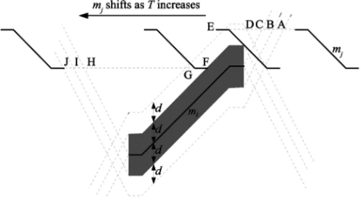
A move consists of three line segments in the time-way di-agram. It has a starting point, an ending point, and two corner points in between (one close to starting point and the other close to the ending point). To simplify later presentations, we define the position of a move (position of as well) as a function of time , in the range between and , as shown in the equa-tion at the bottom of the next page.
During the period from to , is performing and the distance between it and any other hoist cannot be closer than .
Fig. 5. Relations between two moves.
Therefore, if (the shaded area in Fig. 4),
there will be no feasible value for .
If (the point is below ), to ensure safe
distance between the hoists, we must have .
Similarly, if , we must have
.
The constraints in the above three situations for can be summarized as shown below
if if
infeasible if
(10)
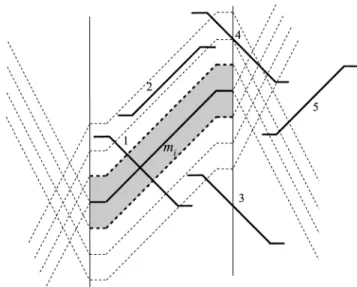
C. Constraints From Move Pairs
We now come back to a pair of moves and in the cycle
( ; ; ; ). If any one
of them is assigned to a hoist, then the hoist assignment of the other is restricted. As shown in Fig. 5, such restrictions may exist between and in the same cycle and between in one cycle and in the next cycle. But they can be handled in the same way.
We consider the two moves in the same cycle first. Based on the discussions in the last subsection, if the hoist assignment constraint between one of the two moves and some point of the other is infeasible, then the cycle length is infeasible. Note that the constraint is in the format of inequality (8), (9), or (10), depending on the relative positions of the move and the point. If the constraints between one move and every point of the other are all feasible, then feasible hoist assignments for this pair of moves exist. In fact, as we will show below, there is no need to consider the constraints between one move and every point of the other.
Fig. 6. Examples of relative positions betweenm and m .
Proposition 2: For a pair of moves and , the hoist assignment variables and satisfy all of the constraints between one move and every point of the other if and only if they satisfy all of the constraints between one move and the starting, ending, and corner points of the other.
Proof: The condition is clearly necessary because if the
constraint between a move and a point of the other is not satis-fied, then the two hoists will violate the safety distance require-ment at the time of that point.
We now prove that the condition is sufficient by considering different cases for the relative positions of a move pair and (e.g., different positions of relative to in Fig. 6). For simplicity, we will refer to the constraint from the relation be-tween a point of one move and the other move as the constraint for that point. This will not cause confusion as there are only two moves involved.
Case 1) the two moves do not overlap in time (e.g., is in position 5 for the example in Fig. 6). If and satisfy the constraint for , the starting point of , then they satisfy inequality (8), with as and
as the point in the formula. That is, is
bounded as follows:
if
if and
if and
Since (i.e., the line segments of are flatter than or with the same slope as the bounding lines on the
right of ), we have for every
point on other than the starting point. Then, if we replace and in the above bounds with and , respectively, the lowerbound will be unchanged or become smaller, the upperbound will be unchanged or become larger, and, hence, will be still within the resulting new bounds. That is, if and satisfy the constraint for the starting point of , they also satisfy the constraints between and all other points on . Therefore, it is enough to consider only the constraint for the start point of . Equivalently, it is enough to consider only the ending point of .
Case 2) the two moves overlap in time. We discuss this case in two more detailed cases.
2.1) the two moves cross each other (e.g., is in po-sition 1 in Fig. 6). This is a definitely infeasible case. Since the two moves cross each other, they overlap in time. Point , the starting point of , is on the left boundary of the overlapping pe-riod. On the right boundary is either or , the ending point of or . If the dis-tance from the point on either boundary to the other move is less than , then the infeasibility is identi-fied by constraint (10) for this point. Otherwise, if is on the right boundary, the two points
and must be on different sides
of due to the crossing. Then, constraint (10) for
the point above requires but
an-other constraint (10) for the point below requires , which indicates infeasibility. Sim-ilarly, if is on the right boundary, then one constraint (10) for and another con-straint (10) for will conflict with each other. Therefore, when the two moves cross each other, the infeasibility can always be identified by the constraints between a move and the starting and ending points of the other.
2.2) the two moves do not cross each other (e.g., is in positions 2, 3, or 4 in Fig. 6). If part of is on the right of the vertical line as in situation 3 or 4 in Fig. 6, the constraint for the point of at the time will also be satisfied for all of the points of on its right, as can be proved in the
same way as for Case 1) (because ). For
the same reason, all of the constraints for the points
outside the two moves’ overlapping period need not be considered. The hoist assignment constraint from the two moves is then defined by the closest vertical distance of the two moves in the overlapping period. Now, we prove that the closest distance between the two moves in the overlapping period is reached at one of the starting, ending, or corner points. Suppose the closest distance occurs between a midpoint on a segment of one move and a midpoint on a segment of the other move, then these two segments of the two moves must be parallel. Then, moving from this point to right (or to the left), the vertical distance between the two parallel line segments is always the closest distance until, and including, the end of one of these two segments. This end of the line segment must be an ending point (or starting point, if moving to the left) or a corner point of a move. Hence, it is sufficient to consider only the constraints for the starting, ending, and corner points.
The above discussions on the sufficiency of the condition have included all possible cases. The proof is complete.
From the proof of Proposition 2, we can see that, for and in the same cycle, it is enough to consider only the constraints between and the start point of if there is no overlapping in time between the two moves ; and if there is overlapping in time between them, it is enough to con-sider only the constraints between each move and the starting, ending, and corner points of the other in the overlapping time period. Altogether, we have the following constraints for the re-strictions between and in the same cycle.
Case 1) Between and the starting point of , if
Case 2) Between and the starting point of , if ,
as shown if if infeasible if if if infeasible if
Case 3) Between and the corner point of , if , as shown in the first equation at the bottom of the previous page.
Case 4) Between and the corner point of
, if , as shown in the first equation at the bottom of the page.
Case 5) Between and the ending point of , if ,
as shown in the second equation at the bottom of the page.
Case 6) Between and the corner point of
, if , as shown in the third
equation at the bottom of the page.
Case 7) Between and the corner point of
, if , as shown in the fourth
equation at the bottom of the page. Case 8) Between and the ending point of , if
, as shown in the fifth equation at the bottom of the page. if if infeasible if if if infeasible if if if infeasible if if if infeasible if if if infeasible if
Case 1) corresponds to the situation where there is no over-lapping in time between the two moves . Cases 2)–8) are for the situations where there is overlapping in time between the two moves.
For the restrictions between in one cycle and in the next cycle , we can get the constraints in the same way. For simplicity, we use to mean “ in the next cycle.”
The case where they do not have overlapping is
similar to case 1) from before, and the constraints can be easily written
We change the sign of this inequality to make it as a constraint on
Similarly, we can obtain constraints for the restrictions be-tween and in all cases. These are listed in Appendix A as Cases a)–h). Case a) corresponds to the situation where there
is no overlapping in time between and .
Cases b)–h) are for the situations where there is overlapping in time between the two moves.
When the cycle length is fixed, for any pair of moves and
( ; ; ; ), a set of
hoist assignment constraints based on the relationship between the two moves can be obtained as discussed before. Note that some of the cases may not be relevant for a particular move pair. According to the relative positions of the two moves, we can list all of the relevant constraints by checking the Cases 1)–h). If any of the constraints is infeasible, then the cycle length is infeasible. Otherwise, it is easy to see that all of the constraints
are in the format . Calculating
and , we can combine these
constraints into one .
Considering all move pairs, we have the following hoist assignment constraints. Each constraint is a “difference con-straint” that sets lower and upperbounds for the difference of two variables
(11) IV. HOISTSCHEDULINGWITH AGIVENCYCLELENGTH
A. Problem Transformation
When the cycle length is given, our problem becomes to check whether this cycle length is feasible. To solve this
problem, we first transform it to a problem of solving a group of difference constraints.
Proposition 3: A cycle length is feasible if and only if a feasible integer solution exists for the group of constraints (7) and (11) corresponding to .
Proof: From the process of deriving the constraints in the
last section, it is obvious that all of the constraints are necessary conditions for a cycle length being feasible. We only need to show that this group of constraints is also sufficient for a cycle length being feasible.
When the constraint group for a cycle length has a feasible integer solution, to prove the cycle length is feasible, we need to show: 1) that every move is assigned to a hoist and 2) that there is a feasible route for each hoist in a complete cycle (i.e., the moves assigned to the same hoist can be feasibly linked in the time-way diagram to form a route for the hoist and the routes of any two adjacent hoists keep at least a safety distance from each other all the time).
1) From an integer feasible solution of constraints (7) and (11), we can get an integer value for each , . Constraint (7) ensures that the values
all satisfy . Therefore, every move is
assigned to one of the hoists for a feasible integer so-lution. Note that different variables may take the same value (i.e., a hoist may be assigned to perform several moves). But the hoist assignment satisfies constraint (11) between any pair of moves (i.e., after performing one of the moves, there is enough time for the hoist to travel to the next move and perform it).
2) Now we show the existence of a feasible schedule by constructing a route for each hoist in the time-way dia-gram and proving the feasibility of these routes. To con-struct the routes, we order all moves in cycle in as-cending order of their starting times. The corresponding
ordered moves are denoted by .
Without loss of generality, we define the moves
performed by hoist to be
where .
For each hoist , we need to prove that there is a feasible route for it to travel for a complete cycle, including the link that crosses the cycle boundary (starts in one cycle and completes in the next) (e.g., from in cycle
to in cycle ). For convenience, we
refer to the move in cycle as in the
current cycle .
We first construct a route for . To construct the route, we only need to construct a link between each adjacent pair of
moves and , . We can
con-struct the link in the following way (see Fig. 7 for illustrations). In the time-way diagram, starting from the ending point of (point ), draw a line downwards with slope , which in-tersects the horizontal line at point . From the starting point of (point ), draw a line downwards with slope , which intersects the horizontal line at point . If the lines and do not intersect above or on the horizontal line as shown in Fig. 7(a), the link is constructed using the
Fig. 7. Hoist route betweenm andm .
intersect at a point above or on the horizontal line as shown in Fig. 7(b), the link is constructed using the two line seg-ments and . If point is overlapped with point or as shown in Fig. 7(c), the link is constructed by connecting the two points and directly. In all of the cases, the link is fea-sible (i.e., the hoist can feasibly travel from to
along the link), because the hoist speeds required on the link segments are all within the maximum empty hoist speed .
To show that this route of does not conflict with the moves assigned to other hoists, we consider any move which is assigned to a hoist . If any part of is in a time interval that contains a move or the sloped link segments on the route of , then from the above route construction method, we know that the move–pair constraints ensure that is at least distance vertically above the route of in this interval. If any part on is in a time interval that contains a horizontal link segment on the route of , then from the individual move constraints, we know that is also at least distance vertically above the route of in this interval. In summary, any move is always at least distance vertically above the route of (i.e., the route of does not conflict with the moves assigned to other hoists). Now, we imagine a path that is exactly distance above the route of and then construct the route for by linking
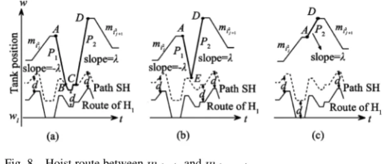
each pair of moves and , (see
Fig. 8 for illustrations). Starting from the ending point of (point ), draw a line downwards with slope , which inter-sects the path at point . From the starting point of
(point ), draw a line downwards with slope , which in-tersects the path at point . If the lines and do not intersect above or on as shown in Fig. 8(a), the link is con-structed using the line segment , path and line segment
. If the lines and intersect at a point above or on as shown in Fig. 8(b), the link is constructed using the two line segments and . If point is overlapped with point or , as shown in Fig. 8(c), the link is constructed by connecting the two points and directly. Clearly, the route of con-structed this way keeps at least distance from the route of because it never goes below path . Similar to the situation for , it can be shown that the route of does not conflict
with moves assigned to hoists .
Imagining a path that is exactly distance above the route of , we can construct the route for in the same way as for . Similarly, we can construct the routes for other hoists, one-by-one, and show that the routes for any adjacent hoists al-ways keep at least a distance of . Now consider the route of
Fig. 8. Hoist route betweenm andm .
, the individual move constraints guaranteed that the moves on the route are all below the line . From the route construction method, we can see that the link between any two moves is always lower than the highest point of the two moves. Thus, the whole route of is below the line . In sum-mary, the routes of the hoists constructed above are all within the vertical range and always keep at least a distance from each other. Therefore, the hoist routes are feasible (i.e., the corresponding cycle length is feasible).
The proof of this proposition provides a method to construct a feasible schedule. Since each move needs to be linked to only one other move on its right in the route of the hoist assigned to them, we only need to construct move links. The number of line segments for each link is proportional to the number of moves of the hoist routes below it. Therefore, the com-putational complexity for constructing a feasible schedule is
.
Note that the route construction method given in the above proof is mainly for showing the existence of a feasible schedule when the group of constraints (7) and (11) has a feasible integer solution. In the resulting hoist routes, however, the empty hoist moves may be unnecessarily long as can be seen from Figs. 7 and 8. With proven existence of a feasible schedule, schedules can actually be constructed differently, in which most links be-tween the loaded moves in the hoist routes can be straight lines. For example, we can modified the schedule constructed in the proof in the following way. Modify the routes of the hoists, one by one from Hoist to Hoist 1: between each pair of adjacent moves assigned to the hoist, let the empty hoist move along a straight line on the time-way diagram; whenever it reaches a point that has a distance of to the route of an adjacent hoist, detour along a path that keeps the safety distance of to the route of that adjacent hoist until it comes back to the straight line. It can be seen that with this modification step, the complexity for constructing the schedule is still .
B. Problem Solution
For a given cycle length, we can construct constraints (7) and (11). By introducing an auxiliary variable , we can trans-form constraint (7) to the following difference constraint:
(12) According to Proposition 3, the hoist scheduling problem with a given cycle length becomes a problem to find whether there exists an integral solution to the corresponding system of differ-ence constraints (11) and (12).
Fig. 9. Constructing a graph for the system of difference constraints.
Such a system of difference constraints can be represented by a weighted directed graph such that the system is feasible if and only if there exists no negative weight cycle in the graph ([20, pp. 602–605]).
The graph , corresponding to constraints (11)
and (12), is as follows. There are nodes in the graph , where is the source node corresponding
to and node corresponds to the decision variable
. The graph contains arcs, each
corresponding to one bound of a difference constraint. Between
and , there are two directed arcs from
to and from to , as shown in Fig. 9(a). The weights of
and are and , respectively. Between
any and ( ; ), there
are also two directed arcs from to and from to
, as shown in Fig. 9(b). The weights of arcs and are and , respectively. If a negative weight cycle exists in the graph , there is no feasible solution for constraints (11) and (12). Otherwise, the total weight of the
shortest path from to is the solution of .
Since all ’s are integer, it is guaranteed that the solution is integer.
The problem of determining whether graph has a
negative weight cycle can be solved using the Bellman–Ford al-gorithm (see [20]–[22]). Systems of difference constraints and the Bellman–Ford algorithm have been used to solve some other scheduling problems. For example, [16] used a system of dif-ference constraints, with move starting times as variables, to check the feasibility of a given sequence of moves for a single hoist. Reference [23] used a modified Bellman–Ford algorithm to minimize the cycle length for a given robot route.
The following is a procedure, based on the Bellman–Ford al-gorithm, for solving the system of constraints (11) and (12).
Procedure 1: Feasibility Checking
Set and .
Set for .
While : {
If holds for some arcs , then {
For each arc : {
Correct and update if . }
Set . }
Else, {
Stop. ’s are a feasible solution. }}
There is a negative cycle and the constraint system is infeasible.
The computational complexity of the algorithm is .
Since , , the complexity of
this procedure is .
V. SPECIALVALUES OF THECYCLELENGTH
Although the cycle length may take any real value between and , some of the values are infeasible (the corresponding schedule is not feasible) and the feasibility changes only at some special values when increases from to . In this section, we identify all of the special values at which the feasibility may potentially change.
Proposition 4: When the cycle length increases from to , the feasibility may change (from infeasible to feasible or from feasible to infeasible) only if there exists a pair of and
( ; ) such that the value of
or corresponding to the cycle length changes.
Proof: For a given cycle length, the feasibility can be
checked by solving constraints (11) and (12). As discussed in Section III-A, constraints (12) are independent of cycle length and are kept unchanged when cycle length changes. Therefore, the feasibility may change only if there is at least one constraint in constraint set (11) changes (i.e., one of the bounds in the constraint changes). Therefore, feasibility may change only if there exists at least one pair of and such that or changes.
Recall that and are obtained by checking the Cases 1)–h) in Section III-C. We first discuss the changes of and
for Case 1) (assume ).
If Case 1) in Section III-C dominates the other cases for , we have
and may change only when
where
Since , and , the cycle
lengths that may cause changes of are
if
Since the cycle length cannot be shorter than the processing time at a station plus the move time to the next station, we have
and the above cycle lengths can be expressed as
if
Fig. 10. SpecialT values corresponding to the changes of L and U as an example.
Similarly, if Case 1) in Section III-C dominates the other cases for , we have
and may change only when
where
Since , and , the cycle
lengths corresponding to the changes of are
if
where and .
In a similar way, for a pair of moves and with , we can find special values of the cycle length corresponding to possible changes of and for all Cases 1)–h). Detailed formulas for these special values are listed in Appendix B.
For each class of the above special cycle lengths, the value
of can be . Therefore, for a pair and , the
total number of these special cycle lengths corresponding to the
changes of and is bounded by .
The example shown in Fig. 10 gives an explanation of the meanings of these special values. The example shows a pair
of moves and for a problem with three hoists.
Imagine we increase the cycle length continuously, will move to the left with respect to . At the beginning, the starting point of is to the right of point . When the cycle length increases, passes through points , , , and one by one. changes from 2 to 1 when the starting point of
passes through points . Similarly, changes from 1 to 0 and 0 to -1 when the starting point of passes through points and , respectively. When the starting point of passes
through points and , changes from to and to
0, respectively. After its starting point passes through point , enters the shaded region and the corresponding cycle length becomes infeasible. At this time, we have
to reflect the infeasibility.
When cycle length increases further, will leave the shaded region and its ending point passes point . At this time, when
changes from 0 to , we have .
changes from to when the ending point of passes
point . Similarly, changes from to 0, 0 to 1, and 1 to 2 when the ending point of passes points , , and , respectively.
From the above analysis, we know that for this example, the pair of moves and defines a total of 10 special cycle length values, corresponding to points to , respectively.
VI. COMPLETESOLUTION TO THENO-WAITPROBLEM With all of the results of the previous sections, we know that the no-wait multihoist scheduling problem under study can be solved by generating the lowerbound, the upperbound, and all of the special values of the cycle length, and then checking the fea-sibility of these special values in ascending order starting from the lowerbound. As the feasibility may only change at these values, the first feasible value will be the optimal cycle length and the corresponding hoist schedule is an optimal schedule. The overall algorithm to obtain the optimal solution is summa-rized as follows:
Procedure 2: Algorithm to solve the no-wait problem
Read problem data and calculate and .
For : {
. If , the problem is infeasible. stop. }
Calculate the special values for each pair of moves according to the formulas in Section V.
Order all of the special values in ascending order and get rid of the duplicates and the values outside the interval . Call the resulting ordered values “checking points” (cycle lengths)
and name them .
Set .
While : {
Let and calculate and for .
For ; : {
Construct and by checking Cases 1)–h) in
Section III-C. If , is infeasible, set , go back to step . }
Apply Procedure 1 to determine whether there is a feasible solution to the constraints (11) and (12). If it is infeasible, set
, go back to step . Otherwise, is the optimal cycle length; construct an optimal schedule using the method described in Section IV-A; stop. }
All of the checking points are infeasible. Stop; the problem is infeasible.
Fig. 11. No-wait solution for the example.
Proposition 5: The no-wait multihoist cyclic scheduling
problem with fixed processing and transfer times is polynomi-ally solvable.
Proof: Procedure 2 solves the problem because it generates
an optimal hoist schedule when the problem is feasible and it indicates infeasibility otherwise.
In the procedure, for each pair of moves, and , the number of checking points is bounded by . The total number of checking points is then . The complexity of Procedure 1 for checking feasibility of a checking point is . Hence, the complexity to check all of the checking points is . Ordering the special values is completed with
the complexity of before the checking process.
The optimal schedule is constructed with the complexity of after the checking process. Therefore, the computational complexity of the complete algorithm is .
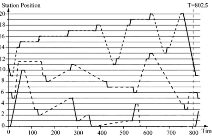
Illustrative example
As an illustrative example, we apply the algorithm to the following three-hoist problem . The system has 20 processing stations and a further station (station 0) for both loading and unloading. The positions of the stations
are , . The position limits for the
hoists on the track are , . The safety
distance between hoists is 1.5. The loaded and empty
hoist speeds are and , respectively. The
time for lifting up or dropping off a part at a station is . The order of stations (the ’s) that the parts visit is . The processing times at the stations, in the above order, are
.
The algorithm takes only 0.025 s (on a Pentium III PC with 750 MHz CPU) to obtain an optimal no-wait schedule with (see Fig. 11). From the results, we can see that the algorithm is very efficient.
To observe the impact of system settings on the optimal cycle length and to demonstrate the efficency of our algorithm in dif-ferent situations, we change the above example data to gen-erate more instances in the following two ways: 1) try different number of hoists from 1 to 5; 2) change the range (the leftmost and rightmost positions) that hoists can travel on the track. The combination of these provides 25 different instances including
TABLE I
RESULTS FOR THEEXAMPLEWITHCHANGEDPARAMETERS
the original one shown above. Table I shows the results of ap-plying the algorithm to these instances. Two numbers are shown for each problem instance. The first number is the resulting optimal cycle length for that case and the second number (in brackets) is the computation time used (in seconds on a Pen-tium III PC with 750-MHz CPU).
From the results, we can see that, in general, the optimal cycle length becomes shorter (e.g., the productivity of the elec-troplating line becomes higher), when the number of hoists in-creases. This is because more hoists mean more resource ca-pacity while the material handling workload in a cycle is fixed. However, when the system has adequate hoists (3 or 4 for this example), adding more hoists will not reduce the optimal cycle length further. In fact, too many hoists may increase the optimal cycle length, as can be seen in the case of 5 hoists with a trav-eling range from 0 to 20, because of the increased interference among them.
The change of the hoist traveling range does not affect the optimal cycle length when the number of hoists is small. With a larger number of hoists, increasing the traveling range by a safety distance (1.5) reduces the optimal cycle length due to relaxed constraints. Furthermore, increasing the range at both ends of the track results in more reduction in the optimal cycle length compared to increasing at one end. The results also in-dicate that increasing the traveling range by one safety distance seems sufficient and a further increase does not affect the op-timal cycle length for this example.
The computation time required increases as the number of hoists increases due to the increasing number of hoist assign-ment options. The change in the hoist traveling range has little impact on the computation time when the number of hoists is not large (up to 3 in this example). With a larger number of hoists, the computation time decreases when the range increases. In any of these cases, however, the computation time never exceeds 0.1 s, confirming that our algorithm is very efficient.
VII. CONCLUSION
In this paper, we have studied the multihoist no-wait cyclic scheduling problem in which the tank processing times and the part move times are fixed parameters, and developed a polynomial algorithm to obtain an optimal schedule with min-imum cycle length. The polynomial solution is based on the following two developments: 1) For the problem with a fixed cycle length, we analyzed the relationship between the part moves and identified a group of hoist assignment constraints. The problem with the fixed cycle length was then transformed to a system of difference constraints on the hoist assignment
variables. The constraint system can then be solved efficiently. 2) a set of special values of the cycle length that might cause feasibility change was derived. The whole problem was then solved by checking the feasibility of these special values in ascending order. The computational complexity of the complete algorithm is . An example was given demonstrating that the algorithm is very efficient.
APPENDIXA
CONSTRAINTS FOR THERESTRICTIONSBETWEEN INONE CYCLE AND IN THENEXTCYCLE(DENOTED AS ) Case a) Between and the starting point of , if
Case b) Between and the corner point of ,
if , as shown in the first equation
at the bottom of the page.
Case c) Between and the corner point of
, if , as shown in the second
equation at the bottom of the page.
Case d) Between and the ending point of , if
, as shown in the third equation at the bottom of the page.
Case e) Between and the starting point of , if ,
as shown in the fourth equation at the bottom of the page.
Case f) Between and the corner point of
, if , as shown in the first equation at
the bottom of the next page. Case g) Between and the corner point
of , if , as shown in the second equation
at the bottom of the next page.
if if infeasible if . if if infeasible if . if if infeasible if . if if infeasible if .
Case h) Between and the ending point of , if
as shown in the third equation at the bottom of the page.
APPENDIXB
SPECIAL VALUES OF THE CYCLE LENGTH THAT MAYCAUSECHANGES OF AND 1) For Case 1) if where if where 2) For Case a) if where if where 3) For Case 2) if if where
4) For Cases 3) and b)
if
if
where
5) For Cases 4) and c)
if if if infeasible if . if if infeasible if . if if infeasible if .
if
where
6) For Cases 5) and d)
if if where 7) For Case e) if if where
8) For Cases 6) and f)
if
if
where
9) For Cases 7) and g)
if
if
where
10) For Cases 8) and h)
if
if
where
REFERENCES
[1] L. Lei and T. J. Wang, “A proof: The cyclic hoist scheduling problem is NP-complete,” in Working Paper 89-0016. Piscataway, NJ: Rutgers Univ., 1989.
[2] L. W. Phillips and P. S. Unger, “Mathematical programming solution of a hoist scheduling program,” AIIE Trans., vol. 28, pp. 219–225, 1976.
[3] W. Song, Z. B. Zabinsky, and R. L. Storch, “An algorithm for sched-uling a chemical processing tank line,” Prod. Planning Control, vol. 4, pp. 323–332, 1993.
[4] J. Liu, Y. Jiang, and Z. Zhou, “Cyclic scheduling of a single hoist in extended electroplating lines: A comprehensive integer programming solution,” IIE Trans., vol. 34, pp. 905–914, 2002.
[5] R. Armstrong, L. Lei, and S. Gu, “A bounding scheme for deriving the minimal cycle time of a single-transporter n-stage process with time-window constraints,” Eur. J. Oper. Res., vol. 78, pp. 130–140, 1994. [6] L. Lei and T. J. Wang, “Determining optimal cyclic hoist schedules in
a single-hoist electroplating line,” IIE Trans., vol. 26, pp. 25–33, 1994. [7] W. C. Ng, “A branch and bound algorithm for hoist scheduling of a circuit board production line,” Int. J. Flexible Manuf. Syst., vol. 8, pp. 45–65, 1996.
[8] H. Chen, C. Chu, and J. M. Proth, “Cyclic scheduling of a hoist with time window constraints,” IEEE Trans. Robot. Autom., vol. 14, no. 1, pp. 144–152, Feb. 1998.
[9] L. Lei, “Determining the optimal starting time in a cyclic schedule with a given route,” Comput. Oper. Res., vol. 20, pp. 807–816, 1993. [10] V. Kats and E. Levner, “A strongly polynomial algorithm for no-wait
cyclic robotic flowshop scheduling,” Oper. Res. Lett., vol. 21, pp. 171–179, 1997.
[11] Y. Crama, V. Kats, V. Van de Klundert, and E. Levner, “Cyclic sched-uling in robotic flowshops,” Ann. Oper. Res., vol. 96, pp. 97–124, 2000. [12] P. Serafini and W. Ukowich, “A mathematical model for periodic scheduling problems,” SIAM J. Discrete Math., vol. 2, pp. 550–581, 1989.
[13] L. Lei and T. J. Wang, “The minimum common-cycle algorithm for cyclic scheduling of two material handling hoists with time window constraints,” Manage. Sci., vol. 37, pp. 1629–1639, 1991.
[14] A. Che and C. Chu, “Multi-degree cyclic scheduling of two robots in a no-wait flowshop,” IEEE Trans. Autom. Sci. Eng., vol. 2, no. 2, pp. 173–183, Apr. 2005.
[15] L. Lei, R. Armstrong, and S. Gu, “Minimizing the fleet size with de-pendent time-window and single-track constraints,” Oper. Res. Lett., vol. 14, pp. 91–98, 1993.
[16] R. Armstrong, S. Gu, and L. Lei, “A greedy algorithm to determine the number of transporters in a cyclic electroplating process,” IIE Trans., vol. 28, pp. 347–355, 1996.
[17] J. B. Orlin, “Minimizing the number of vehicles to meet a fixed periodic schedule,” Oper. Res., vol. 30, pp. 760–776, 1982.
[18] V. Kats and E. Levner, “Minimizing the number of robots to meet a given cyclic schedule,” Ann. Oper. Res., vol. 69, pp. 209–226, 1997. [19] J. Liu and Y. Jiang, “An efficient optimal solution to the two-hoist
no-wait cyclic scheduling problem,” Oper. Res., vol. 53, pp. 313–327, 2005.
[20] T. H. Cormen, C. E. Leiserson, R. L. Rivest, and C. Stein, Introduction
to Algorithms, 2nd ed. Cambridge, MA: MIT Press, 2001. [21] R. Bellman, “On a routing problem,” Quarterly of Applied
Mathe-matics, vol. 16, pp. 87–90, 1958.
[22] R. K. Ahuja, T. L. Magnanti, and J. B. Orlin, Network Flows:
Theory, Algorithms, and Applications. Upper Saddle River, NJ: Prentice-Hall, 1993.
[23] V. Kats and E. Levner, “Polynomial algorithms for scheduling of robots,” in Intelligent Scheduling of Robots and FMS, E. Levner, Ed. Holon, Israel: CTEH, 1996, pp. 77–100.
Yun Jiang received the Ph.D. degree in industrial
engineering from Hong Kong University of Science and Technology (HKUST), Hong Kong, China, in 2003 and the B.S. degree in automatic control from Hua Zhong University of Science and Technology, Wuhan, China, in 1998.
He was a Research Associate and Research Fellow with HKUST and the National University of Singapore (NUS), respectively. Currently, he is an Assistant Professor with Bilkent University, Ankara, Turkey. His research interests include scheduling and planning in production and logistics.
Jiyin Liu received the B.Eng. degree in industrial
automation and the M.Eng. degree in systems en-gineering from Northeastern University, Shenyang, China, in 1982 and 1985, respectively, and the Ph.D. degree in manufacturing engineering and operations management from the University of Nottingham, Nottingham, U.K., in 1993.
Currently he is Professor of Operations Manage-ment in the Business School at Loughborough Uni-versity, Leicestershire, U.K. Prior to joining Lough-borough University, he was with Northeastern Uni-versity and Hong Kong UniUni-versity of Science and Technology, Hong Kong, China. His research interests are in operations planning, scheduling, and supply chain and logistics management. He has published papers in journals such as the European Journal of Operational Research, IIE Transactions, International
Journal of Production Research, Journal of the Operational Research Society, Naval Research Logistics, Operations Research, and Transportations Research.