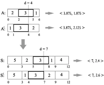
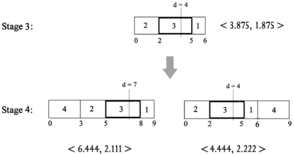
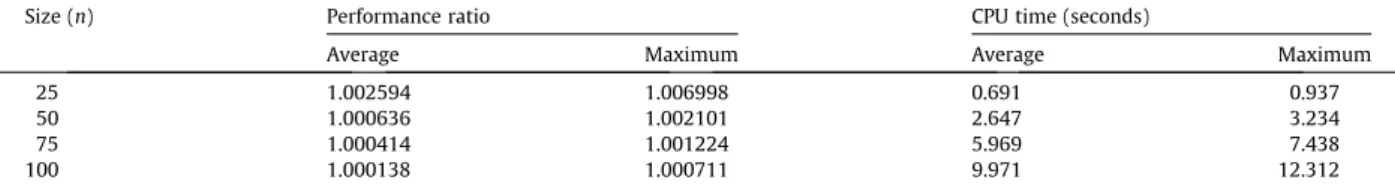
Minimizing weighted mean absolute deviation of job completion times from their weighted mean

Aim: We aimed to determine the frequency of rebound hyperbilirubinemia (RHB) needing treatment and therefrom, to clarify the clinical importance of routinely checking serum

We have analyzed various state-of-the-art methods for impulse noise de- tection and removal, namely Adaptive Median Filter (AMF), Modified Decision Based Unsymmetric Trimmed

It was shown that source memory performance is better for faces with negative be- havioral descriptions than faces that match positive and neutral behavior descriptions (Bell

But unique correction factor as a function of Biot Number, dimensionless time and dimensionless position couldn’t be obtained.. It has been considered to take first

Figure C.4 The Performance of interleavers in convolutional encoded DS-SS for various block lengths, (SNR=10 dB, SIR=2 dB,   0. 5 and block length=300-1400 bits). Table C.3 The

But now that power has largely passed into the hands of the people at large through democratic forms of government, the danger is that the majority denies liberty to

This research is about the relationship between photography and romantic love; The need for 'love' and the need for 'memory photography' are in a way similar; they both serve as

The recently published position paper by the European Heart Rhythm Association, Acute Cardiovascular Care Association, and European Association for Percutaneous Cardiovascular