4
The Impact of Investor Sentiment on the “Leverage Effect”
Semen Son-Turan MEF University
ABSTRACT
With the advent of the Internet and the availability of user search query data on a broader scale, since the early 2000s researchers have started using collective search query information instead of, or, in addition to, traditional investor sentiment proxies. This study examines whether the leverage (bad news) effect, as measured by the EGARCH (1,1) model, changes with the inclusion of a newly emerging sentiment proxy, internet search volume. The sample consists of 14 US companies belonging to the NASDAQ and NYSE Indices and 501 observations of data collected at weekly frequency spanning a nine year period. Empirical findings suggest that, inclusion of the investor sentiment variable has no clear impact on the bad news effect; there is, however, a discernible increase in volatility persistence. The implications of the findings are that the investor sentiment proxy has additional informational content. Behavioral finance theory and the availability and social proof heuristics serve as potential explanations for such findings.
Key words: EGARCH, Investor Sentiment, Leverage Effect, Behavioral Finance, Internet
Search Queries
JEL Classifications: G02, G12
1. INTRODUCTION
1.1. Background and Aim of Study
The time-varying nature of asset returns has been studied since the introduction of the Autoregressive Conditional Heteroskedasticity Model (ARCH) of Engle (1982). Until ARCH-type models were popularized, error terms of ordinary least squares regressions were assumed to display a constant variance (homoskedasticity). Subsequently, various ARCH-family models have emerged like the generalized autoregressive conditional heteroskedasticity, or shortly, GARCH, model (Bollerslev, 1986) and the exponential GARCH (EGARCH) model proposed by Nelson (1991). The latter allows the examination of the impact of the asymmetric effect of good and bad news, which is a major advantage over the GARCH model. The EGARCH model furthermore, shows the “leverage effect”, which refers to a negative correlation between shocks to variance and shocks to returns. If the asymmetry term in the EGARCH conditional variance equation is negative, a negative shock has a greater impact on volatility compared to positive shocks of the same magnitude. The significance of the persistence of negative shocks, or the volatility asymmetry, indicates that investors are more sensitive to negative news than they are to positive news. Another advantage of the EGARCH model is that, contrary to its predecessor the GARCH model, it does not pose any non-negativity restrictions on variance parameters.
Semen Son-Turan, Faculty of Economics, Administrative and Social Sciences, 34396, Istanbul, Turkey, (email: [email protected]), Tel: +90-212-395-3646.
5
Traditional asset pricing theory backed by the efficient market hypothesis (EMH; Fama, 1970), rests on the assumption that a rational decision maker does not take into account the effect of human emotions (in other words, investor sentiment). Behavioral finance literature, on the other hand, which has its roots in the works of Kahneman and Tversky (1979) and Thaler (1980), sees investor sentiment as an essential part of the asset pricing process. As such, behavioral finance researchers do not question the absence or presence of investor sentiment but rather seek to measure and quantify the impact of such.
This study examines how the investor sentiment variable, as proxied by internet search volume (ISV), interacts with the leverage or “bad news” effect, in that it analyzes the size and significance of both variables and the volatility persistence of the base model compared to the base model that includes the ISV variable as a conditional variance variable.
1.2. Conditional Mean Specification
There are numerous ways of calculating the mean expected returns for a security. As the model changes, however, so does the size of the error term. While no common mean specification to be applied universally in asset pricing exists, the CAPM (Sharpe, 1964), the Fama-French 3 factor model (Fama and French, 1992), the consumption based CAPM (Breeden, 1979), and the Arbitrage Pricing model (Chen et al. 1986) can be listed among the most popular models. New models and derivations of older models are still being developed. The popular CAPM introduces the concept of the risk-free rate and states that expected returns equal the risk free rate plus a linear function of its tendency to co-vary with the market portfolio. Since investors are assumed to be rational decision makers, the only risk that needs to be considered is the systematic risk associated with the market portfolio; any other residual idiosyncratic risk can be diversified to a minimum level.
Under the CAPM, the expected return E(Ri) of a given financial asset “i” is presented as: E(Ri,t) = Rf + i (Rm,t − Rf) + εi,t (1.1) where, is the risk-free rate, E(Rm) is the expected return on the market portfolio (i.e., a portfolio of all assets in the economy), εi is the error term, that is assumed to be normally distributed, and i is the sensitivity to systematic risk, which should be compensated by a higher rate of return, equal to the covariance of asset “i” with the market portfolio (the “beta” of the stock).
In the mid-1960s, this model appeared to provide a good explanation of asset prices. However, these explanations received criticism towards the end of the 1970s, with the applications of tests using time-series regressions of stock returns on index returns to generate estimates of stock-specific betas. The development of the CAPM raised the Joint Hypothesis problem, which implies that finding that forecast errors are possibly predictable does not necessarily mean that markets are inefficient. The asset model itself might have been incorrectly specified. An asset-pricing model cannot be tested easily, however, without making the assumption that prices rationally incorporate all relevant available information and that forecast errors are unpredictable.
Fama et al. (1969) tackled the Joint Hypothesis model by using “The Market Model” to capture the variation in expected returns as shown below:
6
Here Rm,t stands for the current overall market return, and i and i are estimated coefficients from a regression of realized returns on stock “i”, Ri,t, on the overall market returns using data before the event. Assuming that captures differences in expected return across assets, εi,t represents the residual idiosyncratic noise.
With the assumption that stock returns should be unpredictable, idiosyncratic noise (the error term) should be uncorrelated across events. This procedure addresses the joint hypothesis problem and isolates the price development of stock “i” from the impact of general shocks to the market.
This study uses the market model in Equation (1.2) to derive the error term, which is modeled through the EGARCH (1, 1) model
1.3. Conditional Variance Specification
ARCH and GARCH models assume that volatility is inherently symmetric. Under the Value Function property proposed by Kahneman and Tversky (1979), however, investors react asymmetrically to good news versus bad news. The EGARCH model of Nelson (1991) addresses this asymmetric response, as illustrated in Equation (1.3):
) log( ) log( 2 1 1 1 1 1 2 t t t t t t (1.3)
Since the left-hand side of the equation is the logarithm of the conditional variance, the positivity constraints imposed upon the model parameters by GARCH are lifted in the EGARCH model. Here, t–1/σt–1 is the leverage effect, occurring when γ<0 (positive news generate less volatility than negative ones), that seeks to capture impacts of positive and negative news shocks on volatility. Asymmetry is present when γ≠0, meaning that the market differentiates between positive and negative news.
Asymmetric response is often described with the “leverage” or “bad news effect” first presented by Black (1976). A drop in the value of a stock (negative return) increases the financial leverage; this makes the stock riskier and thus increases its volatility. Therefore, if we were to price volatility, an expected increase in volatility would raise the required return on equity. Recalling the Value Function property of Prospect Theory, which simply states that individuals assign more value to losses than gains, we can argue that the EGARCH takes account of this very same behavioral phenomenon through incorporating the “bad news” component into its model. This study uses the EGARCH (1, 1) model with lag specification concurrent with the Akaike Information Criterion (AIC; Akaike, 1974).
Volatility models related to equity stocks are often estimated without exogenous variables (Antweiler and Frank, 2004:1260). Some studies, however, include one or more exogenous variables such as employment rates, CPI, home sales (Flannery and Protopapadakis, 2002), T-bill rates (Engle and Patton, 2001), money growth (Geske and Roll, 1983), gold prices and discount rates (Mangani, 2009), and exchange rates (Araghi and Pak, 2012). Brooks et al. (2001) and Depken (2001) use financial variables such as firm size and trading volume. This study does not include any additional exogenous variable in the mean equation but adds ISV as a regressor to the conditional variance equation.
7 1.3.1. Investor Sentiment
As explained in Son-Turan (2014), the search for an understanding of what causes heteroskedasticity present in the error term gave rise to various alternative explanations. One of the most popular of such is the noise trader model by Delong et.al. (1990). The authors borrow the term “noise trader” coined by Kyle (1985), to describe investors who trade on pseudo signals and argue that they deterred arbitrageurs from pushing back prices to their fundamentals, thereby creating “noise trader risk”.
Investor sentiment models are pioneered by Barberis et al. (1998) and Daniel et al. (1998). These models commonly seek to explore the nature of the decision-making process of noise traders and use certain sentiment-based heuristics.
Once the literature reached an understanding that sentiment contributed to the movements of stock prices, researchers started to look for a quantifiable proxy.
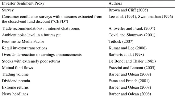
A prominent study by Baker and Wurgler (2007), explains a proxy is an observable phenomenon that serves as an exogenous shock in investor sentiment leading to a chain of events affecting patterns in security pricing. Perhaps it first manifests itself in investor beliefs that could be surveyed, which later on translate into observable trading patterns. Moreover, limited arbitrage causes these demand pressures to lead to mispricings, which in turn may be picked up through benchmarks of fundamental value such as the book-to-market ratio. Mispricing may induce informed responses by insiders, like corporate executives holding inside information and having the ability to act on it to influence the firm’s leverage position. However, as Baker and Wurgler (2007) point out, this chain is prone to confounding influences like surveys not being an exact illustration of how people actually behave compared to their responses. The difficulty of using trades, on the other hand, is that they net to zero (each trade has a buyer and a seller), thus, using this measure means taking a stand on the identity of irrational investors. Also corporate executives may like to change the debt to equity structure of their firms for many reasons other than inside information. Some of the common sentiment proxies are shown in Table 1.1.
Investor Sentiment Proxy Authors
Survey Brown and Cliff (2005)
Consumer confidence surveys with measures extracted from the closed-end fund discount (“CEFD”)
Lee et al. (1991), Swaminathan (1996)
Trade recommendations in internet chat rooms Antweiler and Frank (2004)
Ambient noise level in a futures pit Coval and Shumway (2001)
Pessimistic Media Factor Tetlock (2007)
Retail investor transactions Kumar and Lee (2006)
Over/Underreaction to earnings announcements Barberis et al. (1998)
Stocks with extremely poor returns De Bondt and Thaler (1985)
Mutual fund flows Frazzini and Lamont (2005)
Trading volume Barber and Odean (2008)
Dividend premia Fama and French (2001)
Extreme returns Barber and Odean (2008)
News headlines Barber and Odean (2008)
8
Table 2.2 shows the various proxies traditionally used to measure investor sentiment. We call them traditional in comparison to ISV.
ISV is a powerful proxy since this type of data not only provides insight into one of the long-studied issues in finance, investor sentiment, but also, gives information on how many times a particular search is initiated. As such, it differentiates itself from the other proxies, which are more or less ex post measures of investor actions or suffer from bias.
Apart from seminal economic studies (Askitas and Zimmermann, 2009), finance scholars have only very recently begun to use ISV data based on names or tickers of stock market indices and individual stocks. Several previous studies on stock prices using ISV as investor sentiment proxy are those by Bank et al. (2011); Da et al. (2011); Dimpfl and Jank (2011); Foucault et al. (2011); Vlastakis and Markellos (2012); Bordino et. al. (2012) and Latoeiro et al. (2013).
This study differentiates itself from the previous ones in that it uses EGARCH (1, 1) to determine how the ISV variable interacts with the leverage effect.
2. METHODOLOGY 2.1. Data and Sampling
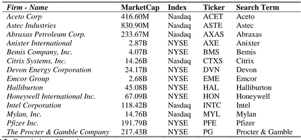
Stocks are systematically selected, based on market capitalization and availability of ISV data, from the two broadest indices representing the US stock market: The NASDAQ Composite (ticker: IXIC) and the NYSE Composite (ticker: NYA). ISV data are obtained from Google Trends, which makes available an index at weekly frequency representing search intensity. The search terms used in this study are the names of the companies. Contrary to studies like Joseph et al. (2011) and Bordino et. al. (2012), ticker-based search queries were not used, resting on the assumption that if an investor already knows the ticker of a company this would imply that she is not an amateur investor and hence, not a noise trader, but rather is an experienced investor who uses rational portfolio diversification and trading techniques. A description of the sample is given below in Tables 2a and 2b:
Firm - Name MarketCap Index Ticker Search Term
Aceto Corp 416.60M Nasdaq ACET Aceto
Astec Industries 830.90M Nasdaq ASTE Astec
Abraxas Petroleum Corp. 233.67M Nasdaq AXAS Abraxas
Anixter International 002.87B NYSE AXE Anixter
Bemis Company, Inc. 004.07B NYSE BMS Bemis
Citrix Systems, Inc. 014.26B Nasdaq CTXS Citrix
Devon Energy Corporation 024.17B NYSE DVN Devon
Emcor Group 002.68B NYSE EME Emcor
Halliburton 045.08B NYSE HAL Halliburton
Honeywell International Inc. 067.09B NYSE HON Honeywell
Intel Corporation 118.42B Nasdaq INTC Intel
Mylan, Inc. 014.76B Nasdaq MYL Mylan
Pfizer Inc. 191.79B NYSE PFE Pfizer
The Procter & Gamble Company 217.43B NYSE PG Procter & Gamble Table 2.2a Description of Sample.
9
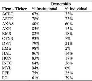
Ownership
Firm - Ticker % Institutional % Individual
ACET 67% 33% ASTE 78% 23% AXAS 40% 60% AXE 85% 15% BMS 82% 18% CTXS 93% 7% DVN 79% 21% EME 98% 2% HAL 86% 14% HON 83% 17% INTC 64% 36% MYL 94% 6% PFE 75% 25% PG 61% 39%
Table 2.2b Description of Sample.
INTC PFE HAL EME DVN
P ISV P ISV P ISV P ISV P ISV
Mean 0.00 0.00 0.00 0.00 0.00 0.00 0.00 0.00 0.00 0.00 Median 0.00 0.00 0.00 0.00 0.00 0.00 0.00 0.00 0.00 0.00 Max 0.17 0.34 0.13 0.87 0.18 1.05 0.24 0.72 0.17 1.02 Min -0.17 -0.20 -0.23 -0.81 -0.43 -0.68 -0.24 -0.78 -0.32 -0.86 Std. Dev 0.04 0.04 0.03 0.14 0.06 0.15 0.05 0.23 0.05 0.26 Skewness -0.10 1.18 -0.81 0.30 -1.14 1.11 -0.19 0.09 -0.67 -0.12 Kurtosis 5.57 13.82 9.65 13.07 9.79 13.14 6.11 3.26 7.23 4.20 J-B 139 2559 979 2127 1073 2256 205 2.10 412 31.14 p 0.00 0.00 0.00 0.00 0.00 0.00 0.00 0.35 0.00 0.00 SSD 0.81 0.85 0.56 10.37 1.73 11.51 1.41 26.24 1.19 32.63
AXAS CTXS HON MYL ASTE
P ISV P ISV P ISV P ISV P ISV
Mean 0.00 0.00 0.00 0.00 0.00 0.00 0.00 0.00 0.00 0.00 Median -0.01 0.00 0.00 0.00 0.00 0.00 0.00 0.00 0.00 0.00 Max 0.53 0.60 0.18 0.52 0.13 0.26 0.31 0.65 0.38 0.61 Min -0.35 -0.69 -0.29 -0.57 -0.21 -0.29 -0.35 -0.78 -0.31 -0.76 Std. Dev 0.10 0.16 0.05 0.09 0.04 0.07 0.05 0.16 0.07 0.17 Skewness 0.73 0.04 -0.49 -0.44 -0.61 0.09 -0.81 0.20 0.04 -0.26 Kurtosis 6.61 5.15 5.79 14.49 6.27 4.22 14.06 6.12 7.14 4.76 J-B 318 96.66 182 2771 255 31.79 2606 207 358 70.39 p 0.00 0.00 0.00 0.00 0.00 0.00 0.00 0.00 0.00 0.00 SSD 5.16 12.25 1.29 4.21 0.71 2.76 1.22 12.40 2.17 15.13 ACET AXE PG BMS
P ISV P ISV P ISV P ISV
Mean 0.00 0.00 0.00 0.00 0.00 0.00 0.00 0.00 Median 0.00 0.00 0.00 0.00 0.00 0.00 0.00 0.00 Max 0.21 0.92 0.30 0.94 0.09 0.55 0.11 0.57 Min -0.29 -0.98 -0.42 -0.95 -0.18 -0.43 -0.13 -0.61 Std. Dev 0.05 0.17 0.05 0.21 0.02 0.13 0.03 0.16 Skewness -0.21 -0.02 -0.72 0.00 -0.88 0.09 -0.09 -0.19 Kurtosis 5.92 7.64 14.74 7.34 10.46 4.10 4.58 3.92 J-B 182 450 2933 394 1226 26.11 52.84 20.62 p 0.00 0.00 0.00 0.00 0.00 0.00 0.00 0.00 SSD 1.45 14.60 1.34 21.93 0.26 8.60 0.49 12.14 Table 2.3 Descriptive Statistics (Transformed Stock Return and ISV Series).
Notes: “Std. Dev”, “J-B”, “p” and “SSD” refer to standard deviation, Jarque-Bera, the J-B associated significance
level and sum of squared differences, respectively. J-B indicates the distribution’s deviation from normality, if
p = 0; the null hypothesis of normality is rejected. Kurtosis measures the peakedness or flatness of the
10
Stock return data are obtained at weekly frequency from Reuters. The number of data points is 501, and the series run from 2004-2013. All data is transformed to log returns, where Rt =ln(Pt)–ln(Pt–1), and tested for stationarity using the Augmented Dickey Fuller test. Table 2.3 provide the descriptive statistics used. As is reported, kurtosis and skewness statistics, also jointly represented by the J-B statistic, show that the data are not normally distributed.
2.2. Pre-Modeling
The definition of the mean equation is the same as Equation (1.2) from section 1.2, where the market is represented by transformed log returns of either NASDAQ or NYSE indices, depending on where the respective stock is listed. The conditional variance equation, on the other hand, models the time varying error term represented by Equation (1.3). This equation is referred to as the “base” model that is used as a reference point to observe the ISV effect. This equation is modified by adding the ISV variable and modeled separately as shown below:
t i t t t t t t ISV ) log( ) log( 21 1 1 1 1 2 (2.4) where the last term represents the ISV variable and is the bad news parameter.
Applying ARCH-type models requires detecting whether ARCH effects are present in the residual of an estimated model. This testing procedure was originally devised by Engle (1982) and is similar to the Lagrange Multiplier (LM) test for autocorrelation. Brooks (2002) explains the procedure for testing for ARCH effects for pre-testing as follows:
Run any postulated linear regression.
Square the residuals, regress them on q own lags (run regression) and obtain R2
. The test statistic is defined as TR2
(the number of observations multiplied by the coefficient of a multiple correlation) from the last regression and is distributed as χ2 with q degrees of freedom.
The null and alternative hypotheses are: H0 : γ1=0 and γ2= 0 and… γq = 0
H1 : At least one of γ1≠0 and γ2≠0 and… γq≠0
Another indicator of conditional heteroskedasticity is Kurtosis, which is a measure of whether the data are peaked or flat relative to the benchmark normal distribution. The kurtosis of normal distribution is 3, values above 3 (defined as leptokurtic, a feature generally associated with financial time series), indicate that a distribution has fatter tails and the chance of extreme outcomes is greater compared to a normal distribution.
2.3. Post-Modeling
To determine whether the applied EGARCH model fits the data, the residuals of the model need to be controlled for autocorrelation and partial autocorrelation functions as well as heteroskedasticity (arch effects). If any of the aforementioned is present, this implies that the EGARCH (1,1) should be modified or replaced.
11
A practical statistic to detect serial correlation is the Durbin Watson (“DW”). The DW, however has its shortcomings, in that it only measures first-order serial correlation (the linear relation between adjacent residuals from the regression equation). A rule-of-thumb: if the DW is very close to 2 no serial correlation is present, and if it is below (above) 2 then a potential positive (negative) correlation may be present.
Another test that overcomes the shortcomings of the DW statistic is the Ljung - Box Q statistic for higher order serial correlation detection. Defined as:
) /( ) 2 ( 1 2 k T r T T Q s k k LB
(2.5)where, T is the sample size, rk
2
is the sample autocorrelation at lag k and s is the number of lags being tested. If the test statistic is bigger than the chi-squared distribution with s degrees of freedom set at a certain significance level, then we reject the null hypothesis.
The null hypothesis of this test is that there is no serial correlation in the residuals up to a specified order (s), specified below as:
H0: rk =0 and k=1,.., s (the data is independently distributed)
H1: rk ≠0 for at least one k =1,.., s (the data displays serial correlation), where rk is the k-th autocorrelation.
Heteroskedasticity tests (Engle’s LM) as outlined above for the residuals of the EGARCH equations are also administered post-modeling.
Tables 2.4 and 2.5 exhibit the EGARCH model outputs and pre- and post-modeling diagnostics of residuals, respectively
3. EMPIRICAL FINDINGS 3.1. Analysis of Results
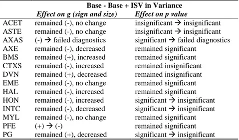
Consider the inclusion of ISV effects as shown in Table 3.6: the sign, size, and significance of the bad news variable g, the EGARCH (1,1) model, and subsequent diagnostic tests reveal that only 28.57% of the total sample (ACET, ASTE, EME, MYL) experienced no change with respect to these three dimensions, where, as depicted in Table 2.2a, 75% of this sample belongs to the NASDAQ Index and represents both large and medium-cap companies. The percentage of institutional ownership, too, is mixed, ranging from 67% to 94% as shown in Table 2.2b. In terms of the significance, only 71.14% of the sample experienced no change with the inclusion of the ISV. Only the significance level of the bad news variable for the remaining companies either turns insignificant (HON, INTC, PG) or the model fails residual diagnostic testing due to autocorrelation still being present in residuals (AXAS). For two of these aforementioned companies (INTC and PG), the ISV variable is significant and positive. For the majority of the sample the bad news term has a negative sign and is significant at 5% in both models. This result indicates that negative shocks lead to higher subsequent volatility than positive shocks.
In light of these findings, the results are mixed, and no clear pattern that could aid in generalization of the impact of ISV on the bad news effect emerges.
12 Base w p a p g p b p ACET -0.33 0.00 0.09 0.02 -0.03 0.19 0.96 0.00 ASTE -4.75 0.04 0.15 0.08 -0.06 0.23 0.21 0.58 AXAS -0.48 0.00 0.20 0.00 -0.07 0.01 0.93 0.00 AXE -0.19 0.00 0.13 0.00 -0.06 0.00 0.98 0.00 BMS -6.54 0.00 0.20 0.03 0.13 0.04 0.15 0.34 CTXS -4.59 0.06 0.11 0.18 -0.06 0.27 0.30 0.41 DVN -0.24 0.01 0.10 0.00 0.03 0.21 0.98 0.00 EME -0.42 0.00 0.16 0.00 -0.06 0.00 0.95 0.00 HAL -0.74 0.04 0.11 0.02 -0.09 0.02 0.90 0.00 HON -0.27 0.03 0.17 0.00 -0.05 0.04 0.98 0.00 INTC -0.84 0.03 0.07 0.14 -0.10 0.00 0.89 0.00 MYL -0.43 0.00 0.18 0.00 -0.08 0.00 0.95 0.00 PFE -2.71 0.00 0.26 0.00 0.14 0.00 0.65 0.00 PG -10.69 0.00 0.36 0.00 0.12 0.05 0.30 0.12
Base + ISV in variance
w p a p g p b p ACET -0.26 0.01 0.08 0.00 -0.03 0.15 0.97 0.00 ASTE -5.78 0.00 0.22 0.03 -0.06 0.27 0.05 0.83 AXAS -9.63 0.00 0.33 0.00 0.02 0.20 0.89 0.00 AXE -0.19 0.00 0.13 0.00 -0.07 0.00 0.99 0.00 BMS -5.49 0.00 0.26 0.01 0.15 0.01 0.30 0.01 CTXS -11.05 0.00 0.02 0.76 -0.08 0.09 0.70 0.00 DVN -0.17 0.03 0.09 0.00 0.02 0.43 0.99 0.00 EME -0.41 0.00 0.16 0.00 -0.06 0.02 0.96 0.00 HAL -0.88 0.02 0.12 0.02 -0.11 0.01 0.87 0.00 HON -0.27 0.02 0.17 0.00 -0.04 0.16 0.98 0.00 INTC -0.78 0.01 0.05 0.21 -0.06 0.08 0.90 0.00 MYL -0.43 0.00 0.18 0.00 -0.08 0.00 0.95 0.00 PFE -0.62 0.01 0.16 0.00 -0.05 0.05 0.93 0.00 PG -0.66 0.01 0.17 0.00 0.01 0.83 0.93 0.00 Table 2.4 Modeling Output – Base and with ISV in Variance.
PRE-MODEL POST- MODEL
OLS ARCH NORMALITY EGARCH ARCH NORMALITY
Obs*R2 Prob. χ2 Kurtosis J-B p Obs*R2 Prob. χ2 Kurtosis J-B p
INTC 028.31 0 05.57 0138.78 0 7.61 0.47 04.25 034.08 0 PFE 017.8 0.02 09.64 0979.37 0 6.61 0.58 05.49 131.36 0 HAL 049.29 0 09.79 1073 0 3.13 0.93 04.15 035.22 0 EME 115.79 0 06.11 0205.12 0 6.73 0.56 04.71 082.33 0 DVN 096.85 0 07.23 0412 0 5.3 0.73 03.53 006.08 0.05 AXAS 045.35 0 06.61 0318 0 3.94 0 04.7 060.81 0 CTXS 036.86 0 05.79 0182.44 0 3.6 0.89 05.15 102.92 0 HON 085.25 0 06.27 0254.52 0 5.95 0.65 03.97 018.17 0 MYL 116.26 0 14.06 2605.6 0 2.58 0.96 07.66 484.8 0 ASTE 030.26 0 07.14 0357.6 0 3.07 0.93 11.36 014.99 0 ACET 016.83 0.03 05.92 0181.88 0 7.37 0.5 06.71 295.1 0 AXE 033.77 0 14.74 2933.09 0 4.22 0.84 08.64 670.24 0 PG 028.88 0 10.46 1226.5 0 7.83 0.45 04.14 029.25 0 BMS 020.18 0.01 04.58 0052.84 0 4.39 0.82 06.77 298.5 0 Table 2.5 Pre- and Post- Modeling Residual Diagnostics.
Notes: The shaded area denotes companies that did not pass final residual testing. “J-B” stands for the
Jarque-Bera statistic, “p” the associated p-value, “Obs*R2” the observed R-squared. The Chi-Square test has the null
hypothesis “there is no significant difference between the expected and observed result”, thus the associated probability (“Prob”), at the target 5% significance level, is not rejected if smaller than 0.05. J-B indicates the distribution’s deviation from normality, if the associated p = 0; the null hypothesis assuming normality is rejected. Kurtosis measures the peakedness or flatness of the distribution.
13
Base - Base + ISV in Variance
Effect on g (sign and size) Effect on p value
ACET remained (-), no change insignificant insignificant ASTE remained (-), no change insignificant insignificant AXAS (-) failed diagnostics significant failed diagnostics AXE remained (-), decreased remained significant
BMS remained (+), increased remained significant CTXS remained (-), increased remained insignificant DVN remained (+), decreased remained insignificant EME remained (-), no change remained significant HAL remained (-), increased remained significant HON remained (-), increased significant insignificant INTC remained (-), decreased significant insignificant MYL remained (-), no change remained significant PFE (+) (-) remained significant PG remained (+), decreased significant insignificant Table 3.6 Leverage Effect and its Relation to ISV in Variance.
The analysis of volatility persistence, that is how long a shock to stock returns takes to die out, as indicated by the GARCH coefficient β, is shown in Table 3.7 below. The table also provides the half-life of volatility shocks, as shown by Lamoureux and Lastrapes (1990), measuring how long it takes for a shock to the conditional variance to reduce to half its original size.
Volatility Persistence Half-Life (weeks)
Base Base + ISV Base Base + ISV
ACET 0.96 0.97 15.93 20.76 ASTE - - - - AXAS 0.93 0.89 10.21 06.18 AXE 0.98 0.99 45.44 47.53 BMS - 0.30 - 00.57 CTXS - 0.70 - 01.95 DVN 0.98 0.99 27.99 46.56 EME 0.95 0.96 15.03 16.09 HAL 0.90 0.87 06.25 05.13 HON 0.98 0.98 37.24 37.79 INTC 0.89 0.90 06.00 06.39 MYL 0.95 0.95 14.45 14.60 PFE 0.65 0.93 01.64 09.82 PG - 0.93 - 10.06
Table 3.7 Volatility Persistence and Half-Life of Shocks toVolatility.
Notes: Blank spaces are due to values above the 5% significance level.
4. CONCLUSION
4.1. Discussion and Implication of Findings
This study tested the hypothesis that inclusion of investor sentiment proxy in the form of internet search volume, obtained through Google Trends, has an impact on the leverage effect. The results of this research confirmed this hypothesis; investors assign greater value to bad news than to good news. Kahneman and Tversky’s (1979) Prospect Theory explains the asymmetric reaction, where the value function is stated to be normally concave for gains,
14
commonly convex for losses, and is generally steeper for losses than for gains. Thus, investors are relatively more sensitive to bad news.
Social psychologists Amos Tversky and Daniel Kahneman explain that when judging the probability of uncertain events people often resort to heuristics, or “mental shortcuts”, which are less than perfectly correlated with the variables that actually determine the event’s probability. One such heuristic is the availability heuristic that may serve as a possible explanation for investor behavior. The availability heuristic is also called “associative distance”, where a person could estimate the likelihood of an event by assessing the ease of the mental operation of retrieval, construction, or association (Tversky and Kahneman, 1973). Investors may be apt at recalling much faster how they felt when they heard about bad news and may associate this experience with a higher probability of occurring again in the future. Furthermore, social contagion theory (Christakis and Fowler, 2013) establishes that emotions, such as fear or happiness, spread between people in direct contact, and, there is an increasing number of studies on social networks which find that for instance Facebook users are affected by each other’s status changes (Coviello et. al., 2014). Since the sentiment data provided in this study originate from the world’s largest search engine Google, investors searching for company information may be influenced by the “auto fill” feature, as well as by Google’s ranking algorithm whereby highly ranked web pages generally have higher visibility to people. Behavioral finance researchers label this phenomenon the “social proof heuristic” (Cialdini, 1984). It essentially explains that when agents are unsure about what to do, they look around for social clues (Hedström and Swedberg, 1998). All these findings and explanations challenge the EMH, since the latter rules out the existence of market bias. The empirical findings establish no direct link between the bad news variable and ISV variable, in the sense that inclusion of ISV as an exogenous variable does not affect the bad news variable in any way (sign, size, or significance level). In other words, the ISV variable has different information content and provides additional explanatory power to the model. Upon inclusion of ISV in the conditional variance equation, both, the volatility persistence and the half-life of volatility shocks increase. Thus, volatility takes a longer time to revert to its mean levels. These results do not differ according to the size, the ownership structure, or the benchmark index of a company. The results can be interpreted as the effect of the investors’ uncertainty about the future and explained with the bounded rationality of human beings and their resort to mental shortcuts, which may not necessarily lead them to correct conclusions about the outcomes of events.
This research yields significant contributions to the literature in that it analyzes how a relatively new investor sentiment proxy interacts with asymmetric effects of stock return volatility. Future research may further investigate the relationship with ISV and traditional sentiment variables in terms of their effect on the variance of stock price returns and their persistence.
REFERENCES
Akaike, H. (1974). A new look at the statistical model identification. IEEE Transactions on Automatic Control, 19 (6), 716-723.
15
Antweiler, W. and M.Z. Frank (2004). Is all that talk just noise? The information content of internet stock message boards. The Journal of Finance, 59 (3), 1259-1294.
Araghi, M.K. and M.M. Pak (2012). Assessing the Exchange Rate Fluctuation on Tehran's Stock Market Price: A GARCH Application. International Journal of Management and Business Research (IJMBR), 2(2), 95-107.
Askitas, N. and K. Zimmermann (2009). Google econometrics and unemployment forecasting. Applied Economics Quarterly, Duncker & Humblot, Berlin, 55 (2), 107-120.
Baker, M. and J. Wurgler (2007). Investor sentiment in the stock market. Journal of Economic Perspectives, 21, 129-152.
Bank, M., M. Larch and G. Peter (2011). Google search volume and its influence on liquidity and returns of German stocks. Financial markets and portfolio management, 25 (3), 239-264.
Barber, B.M. and T. Odean (2008). All that glitters: The effect of attention and news on the buying behavior of individual and institutional investors. Review of Financial Studies, 21 (2), 785-818.
Barberis, N., A. Shleifer, and R. Vishny (1998). A model of investor sentiment. Journal of Financial Economics, 49 (3), 307-343.
Black, F. (1976). The pricing of commodity contracts. Journal of financial economics, 3 (1), 167-179.
Bollerslev, T. (1986). Generalized autoregressive conditional heteroskedasticity. Journal of Econometrics, 31 (3), 307-327.
Bordino, I., S. Battiston, G. Caldarelli, M. Cristelli, A. Ukkonen and I. Weber (2012). Web search queries can predict stock market volumes. PloS one, 7 (7), e40014.
Breeden, D.T. (1979). An intertemporal asset pricing model with stochastic consumption and investment opportunities. Journal of financial Economics, 7 (3), 265-296.
Brooks, R.D., R.W. Faff and T.R. Fry (2001). GARCH modelling of individual stock data: the impact of censoring, firm size and trading volume. Journal of International Financial Markets, Institutions and Money, 11 (2), 215-222.
Brooks, C. (2002) Introductory Econometrics for Finance. Cambridge, UK: Cambridge University Press.
Brown, G.W. and M.T. Cliff (2005). Investor Sentiment and Asset Valuation.The Journal of Business, 78 (2), 405-440.
16
Chen, N.F., R. Roll and S.A. Ross (1986). Economic forces and the stock market. Journal of business, 383-403.
Christakis, N.A. and H.F. James (2013). Social contagion theory: examining dynamic social networks and human behavior. Statistics in medicine, 32 (4), 556-577.
Coval, J.D. and T. Shumway (2001). Is sound just noise? The Journal of Finance, 56 (5), 1887-1910.
Coviello, L., Y. Sohn, A.D. Kramer, C. Marlow, M. Franceschetti, N.A. Christakis and J.H. Fowler (2014). Detecting emotional contagion in massive social networks. PloS one, 9 (3), e90315.
Da, Z., J. Engelberg and P. Gao (2011). In search of attention. The Journal of Finance, 66 (5), 1461-1499.
Daniel, K., D. Hirshleifer and A. Subrahmanyam, (1998). Investor psychology and security market under‐and overreactions. The Journal of Finance, 53 (6), 1839-1885.
De Bondt, W.F. and R. Thaler (1985). Does the stock market overreact? The Journal of
finance, 40 (3), 793-805.
DeLong, J. B., A. Shleifer, L.H. Summers and R.J. Waldmann, (1990). Positive feedback investment strategies and destabilizing rational speculation. The Journal of Finance, 45 (2), 379-395.
Depken, C.A. (2001). Good news. bad news and GARCH effects in stock return data. Journal of Applied Economics, 4 (2), 313-327.
Dimpfl, T. and S. Jank (2011). Can internet search queries help to predict stock market volatility? CFR Working Paper (No. 11-15).
Engle, R.F. (1982). Autoregressive conditional heteroscedasticity with estimates of the variance of United Kingdom inflation. Econometrica: Journal of the Econometric Society, 987-1007.
Engle, R.F. and A.J. Patton (2001). What good is a volatility model. Quantitative finance, 1 (2), 237-245.
Fama, E.F. (1970). Efficient capital markets: A review of theory and empirical work. The
journal of Finance, 25 (2), 383-417.
Fama, E.F., L. Fisher, M.C. Jensen and R. Roll (1969). The adjustment of stock prices to new information. International economic review, 10 (1), 1-21.
Fama, E.F. and K.R. French (1992). The cross‐section of expected stock returns. Journal of Finance, 47 (2), 427-465.
Fama, E.F. and K.R. French (2001). Disappearing dividends: changing firm characteristics or lower propensity to pay? Journal of Financial economics, 60 (1), 3-43.
17
Flannery, M.J. and A.A. Protopapadakis (2002). Macroeconomic factors do influence aggregate stock returns. Review of Financial Studies, 15 (3), 751-782.
Foucault, T., D. Sraer and D.J. Thesmar (2011). Individual investors and volatility. The Journal of Finance, 66 (4), 1369-1406.
Frazzini, A. and O.A. Lamont (2005). Dumb money: mutual fund flows and the cross-section of stock returns. National Bureau of Economic Research.
Geske, R. and R. Roll (1983). The fiscal and monetary linkage between stock returns and inflation. The Journal of Finance, 38 (1), 1-33.
Hedström, P. and R. Swedberg (1998). Social mechanisms: An analytical approach to social
theory. Cambridge University Press.
Joseph, K., M.B. Wintoki and Z. Zhang (2011). Forecasting abnormal stock returns and trading volume using investor sentiment: Evidence from online search. International
Journal of Forecasting, 27 (4), 1116-1127.
Kahneman, D. and A. Tversky (1979). Prospect theory: An analysis of decision under risk. Econometrica: Journal of the Econometric Society, 263-291.
Kumar, A. and C. Lee (2006). Retail investor sentiment and return comovements. The Journal of Finance, 61 (5), 2451-2486.
Kyle, A.S. (1985). Continuous auctions and insider trading. Econometrica: Journal of the Econometric Society, 1315-1335.
Lamoureux, C.G. and W.D. Lastrapes (1990). Heteroskedasticity in stock return data: volume versus GARCH effects. The Journal of Finance, 45 (1), 221-229.
Latoeiro, P., S.B. Ramos and H. Veiga (2013). Predictability of stock market activity using Google search queries. Working Paper 13-06. Universidad Carlos III de Madrid.
Lee, C., A. Shleifer and R.H. Thaler (1991). Investor sentiment and the closed‐end fund puzzle. The Journal of Finance, 46 (1), 75-109.
Mangani, R. (2009). Macroeconomic effects on individual JSE Stocks: a GARCH representation. Investment Analysts Journal, 69, 47-57.
Nelson, D.B. (1991). Conditional heteroskedasticity in asset returns: A new approach. Econometrica: Journal of the Econometric Society, 347-370.
Sharpe, W. F. (1964). Capital asset prices: A theory of market equilibrium under conditions of risk. The Journal of Finance, 19 (3), 425-442.
Son-Turan, S. (2014). Internet Search Volume and Stock Return Volatility: The Case of Turkish Companies. Information Management and Business Review, 6 (6), 317-328.
18
Swaminathan, B. (1996). Time-varying expected small firm returns and closed-end fund discounts. Review of Financial Studies, 9 (3), 845-887.
Tetlock, P.C. (2007). Giving content to investor sentiment: The role of media in the stock market. The Journal of Finance, 62 (3), 1139-1168.
Thaler, R. (1980). Toward a positive theory of consumer choice. Journal of Economic
Behavior & Organization, 1 (1), 39-60.
Tversky, A. and D. Kahneman (1973). Availability: A heuristic for judging frequency and probability. Cognitive Psychology, 5 (2), 207-232.
Vlastakis, N. and R.N. Markello (2012). Information demand and stock market volatility. Journal of Banking & Finance, 36 (6), 1808-1821.