ESSAYS ON MACROECONOMICS
A Ph.D. Dissertation
by
MUSTAFA ANIL TAS¸
Department of Economics
˙Ihsan Do˘gramacı Bilkent University Ankara
ESSAYS ON MACROECONOMICS
The Graduate School of Economics and Social Sciences of
˙Ihsan Do˘gramacı Bilkent University by
MUSTAFA ANIL TAS¸
In Partial Fulfillment of the Requirements for the Degree of DOCTOR OF PHILOSOPHY IN ECONOMICS
THE DEPARTMENT OF ECONOMICS
˙IHSAN DO ˘GRAMACI B˙ILKENT UNIVERSITY
ANKARA September 2018
ABSTRACT
ESSAYS ON MACROECONOMICS
Ta¸s, Mustafa Anıl
Ph.D., Department of Economics
Supervisor: Prof. Dr. Refet Soykan G¨urkaynak Co-Supervisor: Assist. Prof. Dr. Bur¸cin Kısacıko˘glu
September 2018
This dissertation consists of three essays on macroeconomics. The first essay models the term structure of interest rates in an international framework from a macro-finance perspective. Other essays focus on the Turkish economy. The second essay measures the potential growth rate of the Turkish economy. Finally, the third essay examines the stance of monetary policy in Turkey in the post-2001 period.
In the first chapter, I develop a two-country affine term structure model that accounts for the interactions between the macroeconomic and financial variables of each country. The model features a structural preference side and reduced form macroeconomic dynamics. The economies are connected through covered interest parity. Using this framework, I provide an empirical application of the model using data from the United States and the United Kingdom. I quantify the extent to which economic dynamics in one country explain the other’s nominal term
structure. I find that the variation in the bond yields in each country is explained mostly by domestic factors. The cross-country e↵ects are more prominent in pricing of the U.S. bonds.
In the second chapter, I estimate the potential growth rate of the Turkish economy using a bivariate filter. I define the potential growth as the output growth rate at which selected macroeconomic imbalance indicators do not diverge from their targets. This definition of the potential growth implies results that are substantially di↵erent than those suggested by the Hodrick-Prescott filter. I find that these imbalance indicators would not have deteriorated, had Turkey grown at much lower rates particularly after the Great Recession. I also find that for the last five years, Turkey’s potential growth rate is 3 percentage points below the trend growth rate on average. Finally, the results of this study are consistent with the growth target published in the recently announced economic plan of Turkey.
The third chapter is a joint work with Refet G¨urkaynak, Zeynep Kantur and Se¸cil Yıldırım-Karaman. In this chapter, we present an accessible narrative of the Turkish economy since its great 2001 crisis. We broadly survey economic developments and pay particular attention to monetary policy. The data suggests that the Central Bank of Turkey was a strong inflation targeter early in this period but began to pay less attention to inflation after 2009. Loss of the strong nominal anchor is visible in the break we estimate in Taylor-type rules as well as in asset prices. We also argue that recent discrete jumps in Turkish asset prices, especially the exchange value of the lira, are due more to domestic factors. In the post-2009
period the Central Bank was able to stabilize expectations and asset prices when it chose to do so, but this was the exception rather than the rule.
Keywords: Fiscal Policy, Kalman Filter, Monetary Policy, Potential Growth, Yield Curve
¨
OZET
MAKROEKONOM˙I ¨
UZER˙INE MAKALELER
Ta¸s, Mustafa Anıl Doktora, ˙Iktisat B¨ol¨um¨u
Tez Danı¸smanı: Prof. Dr. Refet Soykan G¨urkaynak 2. Tez Danı¸smanı: Dr. ¨O˘gr. ¨Uyesi Bur¸cin Kısacıko˘glu
Eyl¨ul 2018
Bu ¸calı¸sma, makroekonomi ¨uzerine ¨u¸c makaleden olu¸smaktadır. Birinci makalede, faiz oranlarının vade yapısı uluslararası bir ¸cer¸cevede makro-finans per-spektifiyle modellenmi¸stir. Di˘ger makaleler T¨urkiye ekonomisi ¨uzerinedir. ˙Ikinci makalede, T¨urkiye ekonomisinin potansiyel b¨uy¨ume oranı hesaplanmı¸stır. Son olarak, ¨u¸c¨unc¨u makalede T¨urkiye’de 2001 sonrası para politikası uygulamaları incelenmi¸stir.
Birinci makalede, iki ¨ulkenin makroekonomik ve finansal de˘gi¸skenleri arasındaki etkile¸simi dikkate alan bir afin vade yapısı modeli geli¸stirilmi¸stir. T¨uketici tercihleri yapısal olarak modellenmi¸s ve makroekonomik de˘gi¸skenlerin indirgenmi¸s formda oldu˘gu varsayılmı¸stır. ˙Iki ¨ulke ekonomisi arasındaki ili¸ski ¨ort¨ul¨u faiz haddi paritesi ¨uzerinden kurulmu¸stur. Sonra Amerika Birle¸sik Devlet-leri ve ˙Ingiltere verisi kullanılarak modelin ampirik bir uygulaması yapılmı¸stır. Bir ¨ulkedeki ekonomik dinamiklerin di˘ger ¨ulkenin nominal vade yapısını ne ¨ol¸c¨ude
a¸cıkladı˘gı sayısal olarak g¨osterilmi¸stir. Her ¨ulkenin tahvil getirisinin ¸co˘gunlukla kendi i¸c fakt¨orleriyle a¸cıklandı˘gı ve ¨ulkeler arası etkile¸simin A.B.D. tahvil fiyat-lamasında daha belirgin oldu˘gu bulunmu¸stur.
˙Ikinci makalede, iki de˘gi¸skenli filtre kullanılarak T¨urkiye’nin potansiyel ¨uretim b¨uy¨ume oranı tahmin edilmi¸stir. Potansiyel b¨uy¨ume, se¸cilmi¸s makroekonomik dengesizlik g¨ostergelerini hedeflerinden saptırmayan ¨uretim b¨uy¨ume oranı olarak tanımlanmı¸stır. Bu ¸sekilde tanımlanmı¸s potansiyel b¨uy¨ume, Hodrick-Prescott filtresi kullanılarak yapılan tahminlerden ¸cok farklı sonu¸clar ima etmektedir. Se¸cilmi¸s makroekonomik dengesizlik g¨ostergelerinin bozulmasına yol a¸cmayan b¨uy¨ume oranlarının ¨ozellikle B¨uy¨uk Resesyon’dan sonraki d¨onemde ger¸cekle¸sen oranlardan daha d¨u¸s¨uk oldu˘gu bulunmu¸stur. Son be¸s yılın ortalamasına g¨ore potansiyel b¨uy¨ume oranının trendin 3 y¨uzde puan altında oldu˘gu g¨osterilmi¸stir. Son olarak, bu ¸calı¸smanın sonu¸cları T¨urkiye’nin yeni a¸cıklanan ekonomi modelin-deki b¨uy¨ume hedefiyle tutarlıdır.
¨
U¸c¨unc¨u makale, Refet G¨urkaynak, Zeynep Kantur ve Se¸cil Yıldırım-Karaman ile ortak bir ¸calı¸smadır. Bu makalede T¨urkiye ekonomisinin 2001 krizi son-rası d¨onemi de˘gerlendirilmekte ve iktisadi geli¸smeler ¨ozellikle Merkez Bankası’na vurgu yapılarak aktarılmaktadır. De˘gerlendirilen veri TCMB’nin ¨uzerinde ¸calı¸sılan d¨onemin ba¸sında kuvvetle enflasyon hedefledi˘gini ancak 2009’dan sonra enflasyona atfetti˘gi a˘gırlı˘gın azaldı˘gını g¨ostermektedir. Merkez Bankası’nın en-flasyona kuvvetle tepki vermemesi enflasyon ¨uzerindeki kontrol¨un, dolayısı ile de nominal ¸cıpanın kaybına yol a¸cmı¸stır. Nominal ¸cıpanın kaybı, Taylor tipi ku-rallarda ekonometrik olarak bulunan kırılmada oldu˘gu gibi, menkul kıymet fiy-atlarında da g¨or¨ulmektedir. Makalede d¨oviz kurunda yakın d¨onemde g¨or¨ulen
b¨uy¨uk sı¸cramaların T¨urkiye’deki geli¸smelerden kaynaklandı˘gı da savunulmak-tadır. Yapılan vaka ¸calı¸smasında g¨or¨ulmektedir ki yakın d¨onemde Merkez Bankası beklentileri ve mali piyasaları istedi˘ginde stabilize edebilmekle birlikte, genellikle bunu yapmamayı tercih etmi¸stir.
Anahtar Kelimeler: Getiri E˘grisi, Kalman Filtresi, Maliye Politikası, Para Politikası, Potansiyel B¨uy¨ume
ACKNOWLEDGMENTS
I would like to first and foremost thank Refet G¨urkaynak for his excellent guidance and continuous support throughout all stages of my graduate study. I have learned a lot from him, not only about how to be a good economist, but also about how to be a better person. I am immensely grateful to him.
I have been extremely lucky to have Bur¸cin Kısacıko˘glu who cared so much about my work. I am indebted to him for his patience to my endless questions throughout this work. I would also like to thank Sang Seok Lee for his helpful comments and suggestions. This dissertation would not have been completed without their knowledge and support.
I would like to thank Tarık Kara for inspiring me to pursue an academic career, and also for helping me type this dissertation. I also thank Tanseli Sava¸ser for her valuable suggestions at various stages of this work. I especially thank C¸ a˘gın Ararat, Ozan Ek¸si and Aslıhan Salih for being the examining committee members and providing their insightful comments and suggestions.
I would also like to thank my friends, ¨Omer Faruk Akbal, Alican Ayta¸c, Kemal C¸ a˘glar G¨o˘gebakan, Zeynep Kantur, Seda K¨oymen- ¨Ozer, G¨ulserim ¨Ozcan and Se¸cil Yıldırım-Karaman for making my graduate life enjoyable.
I sincerely thank the rest of the faculty and sta↵ of the Department of Eco-nomics for their support throughout my graduate study. I particularly thank
Nilg¨un C¸ orap¸cıo˘glu and ¨Ozlem Demiral for their help with administrative mat-ters.
Finally, I would like to thank my parents, Yurdanur and Mehmet, my sister, Elif, and my brother-in-law, Sarp for their endless support and encouragement.
TABLE OF CONTENTS
ABSTRACT . . . iii ¨ OZET . . . vi ACKNOWLEDGMENTS . . . ix TABLE OF CONTENTS . . . xiLIST OF TABLES . . . xiii
LIST OF FIGURES . . . xiv
CHAPTER 1: AN INTERNATIONAL MODEL OF THE TERM STRUCTURE . . . 1 1.1 Introduction . . . 1 1.2 The Model . . . 3 1.3 Empirical Application . . . 11 1.4 Results . . . 14 1.5 Conclusion . . . 18
CHAPTER 2: ESTIMATING THE POTENTIAL GROWTH RATE OF THE TURKISH ECONOMY . . . 24
2.2 Model and Data . . . 26
2.3 Results . . . 28
2.4 Conclusion . . . 30
CHAPTER 3: MONETARY POLICY IN TURKEY AFTER CENTRAL BANK INDEPENDENCE . . . 34
3.1 Introduction . . . 34
3.2 A Brief History . . . 36
3.3 Fiscal Policy . . . 41
3.4 Monetary Policy . . . 43
3.4.1 Monetary Policy and Inflation . . . 44
3.4.2 Policy Rate and Policy Stance . . . 45
3.4.3 The Regime Switch in Monetary Policy . . . 47
3.4.4 A Narrative Event Study of Recent Past . . . 50
3.5 Conclusion . . . 54
APPENDICES . . . 73
A Bond Pricing Recursions . . . 73
B The State Space System . . . 77
LIST OF TABLES
1.1 Estimates of model parameters . . . 19 1.2 Variance decompositions of selected U.S. yields at 3-month and
10-year horizons . . . 20 1.3 Variance decompositions of selected U.K. yields at 3-month and
10-year horizons . . . 20
2.1 Estimates of model parameters . . . 32 3.1 Taylor rule estimations for the periods before and after the break 57
LIST OF FIGURES
1.1 Model fit of the U.S. yields . . . 21
1.2 Model fit of the U.K. yields . . . 21
1.3 Model fit of the macroeconomic variables and the forward premium 22 1.4 Impulse responses of selected yields to a one standard deviation shock to the U.S. consumption growth and inflation . . . 22
1.5 Impulse responses of selected yields to a one standard deviation shock to the U.K. consumption growth and inflation . . . 23
1.6 Yield factor loadings . . . 23
2.1 Annualized growth rate of output and selected macroeconomic im-balances . . . 33
2.2 Actual growth rate, trend growth rate and estimated potential growth rates of output . . . 33
3.1 GDP growth rates . . . 58
3.2 Real GDP and trend of real GDP . . . 58
3.3 Current account and budget deficits . . . 59
3.4 Unemployment and labor force participation . . . 59
3.5 Inflation . . . 60
3.6 Inflation and core inflation . . . 60
3.8 Primary spending to GDP ratio . . . 61
3.9 Taxes and spending . . . 62
3.10 Government revenues and expenditures . . . 62
3.11 Inflation target and realized inflation . . . 63
3.12 Primary spending, policy rate and inflation rate . . . 63
3.13 CBRT interest rates and overnight repo interest rates . . . 64
3.14 Interest rates, inflation rate and inflation target . . . 64
3.15 Relationship between the interest rate and inflation rate . . . 65
3.16 Counterfactual interest rates . . . 66
3.17 Events and exchange rate responses . . . 67
3.18 A closer look at December 2013–January 2014 . . . 68
CHAPTER 1
AN INTERNATIONAL MODEL OF THE
TERM STRUCTURE
1.1
Introduction
Understanding the movements in bond yields across countries is a central theme for monetary policy discussions. Central banks control the short-term interest rates and private decision makers mostly care about the longer-term rates. This makes the question of how short end of the yield curve transmits into the long end important. Affine term structure models are useful and tractable devices to answer that question, and have become popular beginning with the work of Duffie and Kan (1996).
Most of the studies in the literature on affine term structure models focus on a single country. The few existing multi-country studies investigate the local and global factors that drive the bond yields of countries. Diebold, Li, and Yue (2008) estimate a four-country affine term structure model in which the bond yields are determined by two country-specific latent factors. Those factors then load on the global counterparts. They show that two global factors are responsible for the
joint movements of the yield curves. Recently, Abbritti et al. (2018) build on Diebold, Li, and Yue (2008) and use a factor-augmented vector autoregression framework to analyze the yields curves of eight economies. Their model includes only latent factors extracted as the principal components from the cross section of yields. They find that global factors explain the dynamics at the long end of the yield curves whereas country-specific factors are important at the short end. These studies assume a unidirectional interaction between the pricing factors such that the global ones a↵ect the local ones but not vice versa. The aim of this paper is not to explore the global factors in the term structure of interest rates but instead to gauge the possible e↵ects of the local factors of one country on the yield curve of the other in a two-country setting.
There are two papers that are close to my study. Spencer and Liu (2010) develop a multi-country macro-finance model in which the United States and aggregate OECD economies form the world economy. They allow for mutual interaction between the economic variables of the United States and the OECD. They look at the e↵ects of the world economic factors on the United States and the United Kingdom economies. Bauer and de los Rios (2012) build an international affine term structure model with macroeconomic factors and impose uncovered interest parity under the risk neutral measure. They restrict their model such that the bond yields are a function of country-specific latent factors. This renders macroeconomic variables and exchange rates unspanned.
My study di↵ers from these papers in several aspects. First, both Spencer and Liu (2010) and Bauer and de los Rios (2012) use an ad hoc pricing kernel as in Ang and Piazzesi (2003) that lacks economic interpretation. I derive it from
a utility function that makes all pricing factors spanned. Second, contrary to Bauer and de los Rios (2012), I impose covered interest parity since I make no restrictions on the risk neutral state dynamics. Covered interest parity accounts for the risk premium in the foreign exchange market. Third, I allow the parity condition to enter into the inflation dynamics of each country, thereby introducing an exchange rate pass-through e↵ect. In this sense, my model can be thought of as the two-country version of Wachter (2006) enriched with a foreign exchange market.
1.2
The Model
I build a two-country representative agent term structure model to explain the nominal government bond yield dynamics in each country, where their economies are connected. The model is semi-structural. I consider an endowment economy in which the preferences are modeled with a constant relative risk aversion type utility function and economies in each country have reduced form dynamics. The infinitely-lived representative agent maximizes the discounted sum of her expected utility. Countries share the same model structure, therefore I present the home country dynamics for ease of notation. Variables and parameters with asterisks belong to the foreign country. The agent’s problem is given by
max {Ct}1t=0 E0 " 1 X t=0 tC 1 t 1 Qt # , (1.1)
where is the time-discounting parameter, is the relative risk aversion and Qt
is an exogenous preference shock.1 The processes for consumption growth and
inflation are exogenous:
ct+1 = µc+ c ct+ c,⇡⇡t+ "c,t+1, (1.2)
⇡t+1 = µ⇡ + ⇡⇡t+ eet+ "⇡,t+1, (1.3)
where ct+1 = log (Ct+1/Ct), "c,t+1 and "⇡,t+1 are normal shocks with standard
deviations c and ⇡, respectively. The variable et in Equation (1.3) is the
ex-change rate forward premium, which will be defined later in the paper. The inclusion of forward premium in the inflation process implies that there is one-period lagged exchange rate pass-through to inflation. Following Bansal and Shaliastovich (2013), I allow inflation to directly feed into consumption growth to capture the interaction between the real and nominal variables.
Following Gallmeyer, Hollifield, and Zin (2005) and Kısacıko˘glu (2016), I model the growth rate of the preference shock as a linear function of the in-novations in consumption growth and inflation with time varying coefficients:
qt+1 =
1
2vart( qt+1) c⌫t( ct+1 Et ct+1) ⇡⌫t(⇡t+1 Et⇡t+1) , (1.4) where qt+1 = log (Qt+1/Qt) and ⌫t is an exogenous AR(1) process:
⌫t+1= ⌫⌫t+ "⌫,t+1, (1.5)
1Augmenting the utility function with a preference shock in this way is equivalent to adding external habit in consumption. See Creal and Wu (2017) for a discussion of this relationship.
where "⌫,t+1 is Gaussian with standard deviation ⌫. The parameters c and ⇡
govern the sensitivity of the growth rate of the preference shock to consumption growth and inflation shocks, respectively. The first term on the right hand side of Equation (1.4) guarantees that the preference shock is a martingale:
Et
Qt+1
Qt
= 1. (1.6)
This assumption cancels out the Jensen’s inequality term induced by the lognor-mal property of the preference shock.
The economies of home and foreign countries are linked through covered inter-est parity. It postulates an equilibrium relationship between the forward premium on the nominal exchange rate and the nominal interest rate di↵erential of any two countries such that no arbitrage opportunities occur. To see why, consider two investment strategies. In the first strategy, the investor deposits 100 units of home currency to a bank for one month and earns domestic interest at maturity. In the second strategy, she converts 100 units of home currency into foreign cur-rency from the spot rate, deposits it at the foreign interest rate for one month and enters a forward contract to get home currency back one month from today at a predetermined rate. These investment strategies should give the same rate of return by the no arbitrage principle. Any return imbalances are instantaneously wiped o↵ by the forward rate.
Let it be the continuously compounded home country short rate, st be the
logarithm of the spot exchange rate expressed as home currency per unit of for-eign currency and ft be the logarithm of the forward exchange rate of the same
maturity with the short rate. Formally, the covered interest parity condition is
ft st = it i⇤t. (1.7)
The left hand side of Equation (1.7) is the forward premium. Following Backus, Foresi, and Telmer (2001), I can decompose the forward premium into expected rate of depreciation and risk premium components:
ft st= (Et[st+1] st) | {z } expected depreciation + (ft Et[st+1]) | {z } risk premium . (1.8)
The risk premium in Equation (1.8) is a degree of bias in the forward rate. If the forward rate is an unbiased measure of expectations, then the risk premium would be zero. This means there are no unforeseen fluctuations in the exchange rate or no risk aversion and hence there is no exchange rate risk to be covered. In this case, the covered interest parity relationship would be equivalent to its uncovered counterpart. In this paper, I use the notation et to denote the forward
premium and allow for deviations from the equilibrium2:
et+1 = it+1 i⇤t+1+ "e,t+1, (1.9)
where "e,t+1 is normal with standard deviation e. The forward premium might
fail to match the interest rate di↵erential when expectations, risk premium or both are hit by a shock. Therefore, the shock to the forward premium can
2See Du, Tepper, and Verdelhan (2018) for a recent analysis of the failures of the covered interest parity.
be interpreted as sum of shocks to the expected rate of depreciation and risk premium.
Equations (1.2), (1.3), (1.5) and (1.9) determine the state of the economy in the home country. All variables except the forward premium are country-specific. The latter is a common factor for both the home and the foreign country. Therefore, I isolate the loadings of the forward premium from those of the country-specific factors through the entire analysis. Let Xt=
ct ⇡t ⌫t 0
be the vector of home country-specific factors. Then, I can write the evolution of the state of the economy in the home country in compact form as follows:
Xt+1 = µ + Xt+ eet+ "t+1, (1.10)
where "t+1 ⇠ N (03⇥1, ⌃), and e are 3⇥ 3 and 3 ⇥ 1 matrices, respectively.
So far I have described the agent’s preferences and the macroeconomy. To study the behavior of the term structure in home and foreign countries, I now characterize the bond prices in both economies. Bonds are priced by imposing the no arbitrage restriction across maturities. The absence of arbitrage implies the existence of a strictly positive random variable, Mt+1, called the stochastic
discount factor, such that the price of an n-period domestic bond is
Pt(n)= Et
h
Mt+1Pt+1(n 1)
i
. (1.11)
Equation (1.11) is called the bond pricing equation that holds for any time period. Since I am pricing nominal bonds, the stochastic discount factor is also nominal. The logarithm of the nominal stochastic discount factor implied by the preferences
in (1.1) is given by
mt+1 = log ct+1+ qt+1 ⇡t+1. (1.12)
Shocks to consumption growth and inflation are two fundamental sources of un-certainty that matter for bond pricing. Du↵ee (2013) shows that the marginal utility in standard power utility models is not volatile enough to explain the average term premium. The inclusion of the preference shock growth with time-varying sensitivity parameters provides a solution to this problem.
The mechanism is as follows. Given a one standard deviation inflation shock, the marginal utility shifts by (1 + ⇡⌫t) standard deviations. The additional
shift comes from the qt+1 term. The change in the marginal utility is amplified
but the rise in the volatility comes from the variation in the exogenous shock, ⌫t.
Any shocks to ⌫talter the response of the preference shock growth to the inflation
shock, leading to an augmented shift in the marginal utility. This variation in the volatility of marginal utility makes the conditional covariance between mt+1
and the bond price time-varying, implying a time-varying term premium. Since ⌫t is the key variable in determining the term premium, it can be interpreted as
a valuation shock.3
The payo↵ of an n-period zero coupon domestic bond is equal to 1 unit of home currency at maturity. Then the price of that bond at time t + n 1 is
Pt+n 1(1) = Et+n 1[Mt+n] . (1.13)
Using (1.13) and the fact that Mtis lognormally distributed, mt+1 can be written in a general form: mt+1= it 1 2 0 t⌃ t 0t"t+1, (1.14)
where t is the time-varying price of risk. The forward premium shock does not
show up in the stochastic discount factor. It will propagate through inflation with a one-period delay. Then the price of risk is affine in the country-specific factors:
t = 0+ 1Xt. (1.15)
The total compensation for risk equals the innovation in the stochastic dis-count factor. In other words, what is priced is the the unexpected change in the marginal utility. Using (1.14) and (1.15), I can write:
mt+1 Et[mt+1] = 0t"t+1
= ( 0+ 1Xt)0"t+1. (1.16)
Using the model implied mt+1 in (1.12), I can express the left hand side of (1.16)
in terms of model parameters:
mt+1 Et[mt+1] = ( ct+1 Et[ ct+1]) (⇡t+1 Et[⇡t+1])
( qt+1 Et[ qt+1])
= ( + c⌫t) "c,t+1 (1 + ⇡⌫t) "⇡,t+1
where H = 2 6 6 6 6 6 6 4 1 0 3 7 7 7 7 7 7 5 and K = 2 6 6 6 6 6 6 4 0 0 c 0 0 ⇡ 0 0 0 3 7 7 7 7 7 7 5 .
Matching the coefficients in (1.16) and (1.17) yields 0 = H and 1 = K. To
complete the components for bond pricing, I need a process for the short rate. I assume that the short rate is affine in the state of the economy:
it= 0+ 10Xt+ 2et. (1.18)
Using Equations (1.12), (1.14) and (1.15) and matching the coefficients in (1.18) I get the model implied loadings for the short rate:
0 = log + 00µ 1 2 0 0⌃ 0 (1.19) 0 1 = 00( ⌃ 1) (1.20) 2 = e. (1.21)
Now, I can rewrite the covered interest parity condition in (1.9) in terms of the state variables: et+1 = 0 ⇤ 0 1 2+ 2⇤ + 0 1 1 2+ 2⇤ Xt+1 ⇤0 1 1 2+ ⇤2 Xt+1⇤ + 1 1 2+ ⇤2 "e,t+1. (1.22) I treat et as a separate state variable and therefore put it into a VAR form. To do
country counterpart. Then Equation (1.22) becomes et+1 = µe+ V0 Xt V⇤0 ⇤Xt⇤+ (V0 e V⇤0 ⇤e) et +V0"t+1 V⇤0"⇤t+1+ Ve"e,t+1, (1.23) where V = 1 1 2+ 2⇤ , V⇤ = 1⇤ 1 2+ 2⇤ , Ve = 1 1 2+ 2⇤ and µe= 0 0⇤ 1 2+ ⇤2 + V0µ V⇤0µ⇤.
I assume that bond prices are exponentially affine in all states of the economy:
Pt(n)= exp (An+ Bn0Xt+ Dn0Xt⇤+ Gnet) , (1.24)
where An and Gn are scalars, Bn and Dn are 3⇥ 1 vectors that satisfy the bond
pricing recursions. Then the zero coupon bond yields are given by
yt(n)= An n B0 n n Xt D0 n n X ⇤ t Gn n et. (1.25)
The derivations of the bond pricing recursions are provided in the Appendix. In the following sections, I will do an application of this model.
1.3
Empirical Application
In this section, I will estimate the model using quarterly data from the United States and the United Kingdom. I treat the former as the home country and
the latter as the foreign country. I use three sets of data. The first data set is from OECD Main Economic Indicators and includes consumption growth and inflation. In particular, I use the annualized growth rate of the seasonally adjusted private final consumption expenditures and the annualized growth rate of the consumer price index. The second data set is from Bloomberg and contains the dollar/pound spot exchange rate and the associated 3-month forward points. The third data set is the set of annualized nominal zero coupon bond yields from Wright (2011). I use the yields of maturities 3-month, 6-month, 1-year, 2-year, 5-year and 10-year. The 3-month yield is the short rate. The sample covers the period from 1987-Q1 to 2007-Q4. All observations are end-of-quarter values.
The growth rate of aggregate consumption and the headline inflation are too volatile to be used for fitting affine term structure models. Following Wright (2011), I smooth those series by applying an exponential weighted moving average filter with a smoothing parameter of 0.75. The valuation shock in each country is an unobservable state variable. I extract them using a standard Kalman filter. That requires a measurement equation that links the observable variables to the state vector and a transition equation that describes the evolution of the state variables. There are 2 macroeconomic and 6 yield series for each country. Hence, the total number of observable variables is 17 including the forward premium. As discussed in the previous section, there are 7 state variables. The measurement equation is Zt+1= ˜ + ˜Xt+1+ ˜⌘t+1, (1.26) ˜ ⌘t+1⇠ N ⇣ 017⇥1, ˜⌦ ⌘
whereZt+1is the vector of observable variables, ˜ is a 17⇥1 matrix, ˜ is a 17⇥7
matrix,Xt+1is the vector of state variables and ˜⌘t+1is the vector of measurement
errors. The transition equation is
Xt+1 = ˜µ + ˜Xt+V ˜"t+1, (1.27) ˜ "t+1⇠ N ⇣ 07⇥1, ˜⌃ ⌘
where ˜µ is a 7⇥ 1 matrix, ˜ is a 7 ⇥ 7 matrix, V is the 7 ⇥ 7 impact matrix and ˜"t+1 is the vector of state shocks. Equations (1.26) and (1.27) are written
in the compact form. The detailed state space representation is provided in the Appendix.
I demean all the variables before estimating the model. This procedure re-duces the number of parameters to be estimated. In particular, I do not estimate the As in Equation (1.25). I add the sample averages after the estimation. The dimension of the problem remains large even after dropping the means. There are 40 parameters to be estimated. The estimation results are sensitive to the initial values of the parameters. The likelihood function does not admit a unique optimum. Therefore, the initial parameter vector must be carefully chosen to en-sure a convergence to a local maximum that is consistent with economic theory. Most of the parameters are initialized with values that are estimated from ordi-nary least squares regressions. The persistence parameters and the conditional variances of the valuation shocks are calibrated to roughly match those of the associated macroeconomic variables. The sensitivity parameters of the growth
rate of the preference shock are set with arbitrary values such that the initial value of the likelihood is at maximum.
1.4
Results
In this section, I will discuss the term structure implications of the model. The estimation results are reported in Table 1.1. Consumption growth and in-flation are highly persistent in both countries. The negative covariance between consumption growth and inflation renders the nominal bonds risky. They are not a good hedge against inflation. This relationship is more prominent is the United States. Any shock to macroeconomic variables will lead to a larger shift in the marginal utility of the agent in the United states since the risk aversion there is higher compared to that in the United Kingdom. The valuation shocks are the only latent variables in the model and are fairly persistent in both countries. They work like the level factor described in Litterman and Scheinkman (1991) to fit the yield curves. The forward premium loads to inflation in each country with opposite signs, as expected. An increase in the forward premium means depreciation of the dollar against pound, which then puts a downward pressure on inflation in the United States.
The model fits of the yields, macroeconomic variables and the forward pre-mium are shown in Figures 1.1, 1.2 and 1.3, respectively. The fit of the yields is excellent across all maturities in both countries. The fit of the forward premium is also perfect since it equals the short rate di↵erentials. The model is successful in fitting the consumption growth and inflation. Although the fitting errors are larger compared to those of the yields, the model is able to track the variations in
these macroeconomic series. The divergence between the fitting performances in yields and the macroeconomic variables is a consequence of the utility function. The model requires a certain level of risk aversion to fit the yields. The implied elasticity of intertemporal substitution is not large enough to fit the macroeco-nomic variables.
The main theme of this exercise is to quantify the extent to which economic dynamics in the United States and in the United Kingdom explain each other’s term structure. I do this by looking at impulse responses and variance decom-positions. The impulse responses of selected yields to a one standard deviation shock to the macroeconomic variables in respective countries are displayed in Figures 1.4 and 1.5. The key to interpret the impulse responses is to understand the response of the short rate at t = 0. In the left panel of Figure 1.4, a one standard deviation shock to the U.S. consumption growth leads to a 1.9 standard deviation increase in the U.S. short rate.
The mechanism is as follows. When the shock hits, consumption growth in-creases by 1 unit. The transition to the short rate operates through two channels. First, consumption growth directly enters into the short rate process. Second, it enters indirectly through the forward premium in Equation (1.22). The net e↵ect is determined by the sign and the magnitude of the associated factor loadings. All factor loadings are shown in Figure 1.6. In pricing of the U.S. bonds, U.S. consumption growth dominates all other factors and the e↵ect of forward pre-mium is almost zero. The economic interpretation is as follows. After the shock arrives, since consumption growth is persistent, the agent knows that consump-tion will keep growing and demand for bonds will decrease. Bond prices go down
and yields rise. The short rate and other yields gradually come to a new steady state around 0.6 units in 100 periods.
Inflation enters into the short rate process through the same channels. In the right panel of Figure 1.4, a one standard deviation shock to the U.S. inflation leads to a 0.4 standard deviation increase in the U.S. short rate initially. In the next period, consumption growth falls as a response to inflation. Then the short rate plummets because of the dominance of consumption growth in determining the yields. The intuition is as follows. When the shock hits, the agent knows that the growth rate of her consumption will fall in the following period. That is, her marginal utility will be higher. Then the demand for bonds will increase to smooth consumption. This leads to a drop in the yields. The new steady state occurs around 0.7 units for all yields.
The impulse responses of the U.K. yields to a one standard deviation shock to the U.K. factors are weaker compared to the U.S. case. This is mainly due to the lower sensitivity of the U.K. consumption growth to U.K. inflation compared to the U.S. counterpart.
The impulse responses are similar across maturities. The dashed lines repre-sent the cross-country e↵ects. The impact of the U.S. factors in pricing of the U.K. bonds is near zero. Conversely, the U.K. factors have a substantial e↵ect on the U.S. bond yields. In the left panel of Figure 1.5, a one standard deviation shock to the U.K. consumption growth leads to a 0.3 standard deviation decrease in the U.S. short rate in 20 periods. This level is achieved in 5 periods for the 10-year U.S. yields. In the right panel of Figure 1.5, a one standard deviation shock to the U.K. inflation leads to a steady state of 0.4 standard deviation increase
in the U.S. short rate. The 10-year U.S. yields increase up to 0.5 units. The reason behind this interaction is the dominance of the U.K. consumption growth in pricing of the U.S. bonds.
A caveat of the model is that any shocks to the macroeconomic variables are reflected in the expected short rates. Only the shocks to the latent variables, ⌫t
and ⌫⇤
t, move the term premium. The reason is that the valuation shocks are
ex-ogenous to the model, and thus they do not respond to any of the macroeconomic variables.
The variance decompositions of selected U.S. and U.K. yields are presented in Tables 1.2 and 1.3. The variation in the U.S. short rate is explained mostly by the U.S. consumption growth in the short run. In the long run, the U.S. inflation explains 38.8 percent of that variation. The dominance of the U.S. consumption growth declines as maturity increases. The U.S. inflation retains its explanatory power and the U.S. valuation shock have a mild contribution to the variation in the 2-year and 10-year U.S. yields. The U.K. consumption growth explains a significant portion of the variation in the U.S. yields in the long run at all maturities reaching up to 8.4 percentage points. The variation in the U.S. yields can be roughly attributed to the U.S. macroeconomic factors in general. This is not the case for the U.K. bonds. The U.K. consumption growth is dominant at the short end of the U.K. yield curve whereas the U.K. valuation shock explains almost all the variation in the long end.
1.5
Conclusion
In this paper, I proposed a two-country affine term structure model enriched with macroeconomic factors to analyze the nominal bond yield dynamics in each country. The countries are connected through covered interest parity. This joint framework allows me to figure out the cross-country factors in determination of the yields. The model is applicable to any two countries that have similar characteristics. I estimated the model using data from the United States and the United Kingdom. I found that the U.S. yields are mainly determined by the U.S. macroeconomic factors. The short end of the U.K. yield curve is explained mostly by the U.K. consumption growth and the long end is controlled by the U.K. latent factor. The e↵ect of the U.K. consumption growth is notable in determination of the U.S. yields.
The model can be improved in several directions. The limitations posed by reduced form economic dynamics could be overcome by adopting a structural model incorporating capital flows. Expectations could be modeled accordingly. Furthermore, the computational issues arising in the estimation process would make a Bayesian approach more reliable. I leave them for future research.
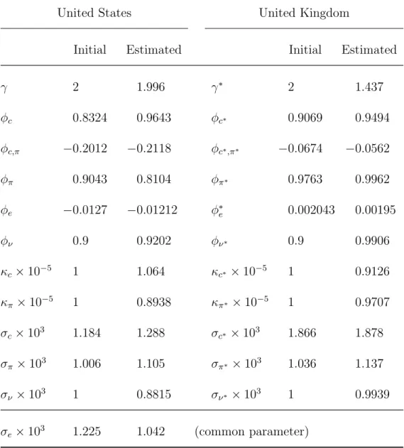
Table 1.1: Estimates of model parameters.
United States United Kingdom
Initial Estimated Initial Estimated
2 1.996 ⇤ 2 1.437 c 0.8324 0.9643 c⇤ 0.9069 0.9494 c,⇡ 0.2012 0.2118 c⇤,⇡⇤ 0.0674 0.0562 ⇡ 0.9043 0.8104 ⇡⇤ 0.9763 0.9962 e 0.0127 0.01212 ⇤e 0.002043 0.00195 ⌫ 0.9 0.9202 ⌫⇤ 0.9 0.9906 c ⇥ 10 5 1 1.064 c⇤⇥ 10 5 1 0.9126 ⇡ ⇥ 10 5 1 0.8938 ⇡⇤ ⇥ 10 5 1 0.9707 c⇥ 103 1.184 1.288 c⇤⇥ 103 1.866 1.878 ⇡ ⇥ 103 1.006 1.105 ⇡⇤⇥ 103 1.036 1.137 ⌫ ⇥ 103 1 0.8815 ⌫⇤⇥ 103 1 0.9939 e⇥ 103 1.225 1.042 (common parameter)
Table 1.2: Variance decompositions of selected U.S. yields at 3-month and 10-year horizons.
U.S. 3-Month Yield U.S. 2-Year Yield U.S. 10-Year Yield
Shocks Q1 Q40 Q1 Q40 Q1 Q40 U.S. Consumption 95.9% 55.6% 72.3% 50.6% 47.9% 44.6% U.S. Inflation 1.6% 38.8% 12.7% 40.4% 32.5% 40.8% U.S. Latent 2.5% 0.6% 15.0% 3.3% 16.5% 4.4% U.K. Consumption 0.0% 4.2% 0.0% 4.9% 2.7% 8.4% U.K. Inflation 0.0% 0.2% 0.0% 0.2% 0.1% 0.1% U.K. Latent 0.0% 0.5% 0.0% 0.7% 0.3% 1.7% Forward Premium 0.0% 0.0% 0.0% 0.0% 0.0% 0.0%
Table 1.3: Variance decompositions of selected U.K. yields at 3-month and 10-year horizons.
U.K. 3-Month Yield U.K. 2-Year Yield U.K. 10-Year Yield
Shocks Q1 Q40 Q1 Q40 Q1 Q40 U.S. Consumption 0.0% 0.0% 0.0% 0.0% 0.0% 0.0% U.S. Inflation 0.0% 0.0% 0.0% 0.0% 0.0% 0.0% U.S. Latent 0.0% 0.0% 0.0% 0.0% 0.0% 0.0% U.K. Consumption 82.4% 78.8% 44.2% 23.1% 4.0% 1.5% U.K. Inflation 13.1% 9.4% 5.2% 2.8% 0.0% 0.8% U.K. Latent 4.5% 11.8% 50.6% 74.0% 96.0% 97.7% Forward Premium 0.0% 0.0% 0.0% 0.0% 0.0% 0.0%
Figure 1.1: Model fit of the U.S. yields.
Figure 1.3: Model fit of the macroeconomic variables and the forward premium.
Figure 1.4: Impulse responses of selected yields to a one standard deviation shock to the U.S. consumption growth and inflation. The responses are in terms of the standard deviation of the associated shock.
Figure 1.5: Impulse responses of selected yields to a one standard deviation shock to the U.K. consumption growth and inflation. The responses are in terms of the standard deviation of the associated shock.
CHAPTER 2
ESTIMATING THE POTENTIAL GROWTH
RATE OF THE TURKISH ECONOMY
2.1
Introduction
Turkish economy has grown by 7.3 percent year-on-year in the first quarter of 2018. This paper evaluates the stance of this number after calculating the potential growth rate according to which it can be judged. The conventional definition of potential growth is the growth rate of output that is consistent with stable inflation. I depart from this usual definition by using other measures of imbalances instead of inflation.
From the production function perspective, potential growth is the growth rate attained with normal use of the factors of production. The normal levels of some of these factors, such as capital and total factor productivity, are usually proxied with their respective Hodrick-Prescott trends. Calculation of the normal level of labor may include the estimation of a Phillips curve. Trend is a statistical concept, whereas potential is an economic term. Economists believe that in the long run, potential output will converge to the trend. They do not have to follow
the same path. Using the Hodrick-Prescott filter at any stage of the potential output or potential growth calculation will result in an unreliable estimate. My definition of potential growth has an influence not only on the labor but also on the other components of a production function.
I employ a bivariate filter that accounts for certain macroeconomic imbalances to estimate the potential output growth for Turkey. Since I merely ask a growth question, I confine my analysis to estimating the potential growth directly. There are a number of papers that have used multivariate filtering methods to estimate the potential output and potential growth in Turkey. ¨Ozbek and ¨Ozlale (2005), Kara et al. (2007), ¨O˘g¨un¸c and Sarıkaya (2011), Blagrave et al. (2015) and Andı¸c (2018) are some examples. All of these papers have considered inflation as the single imbalance indicator that identifies the output gap.
Figure 2.1 shows the annualized growth rate and selected imbalance indicators for Turkey. High growth rates are associated with high current account deficits and increased credit demand. Growth fueled by excessive borrowing cannot be sustainable. Therefore, any potential growth rate that is estimated by ignoring sustainability cannot be potential. My study renames the sustainable growth as the genuine potential growth and resembles the work of Alberola, Estrada, and Santab´arbara (2014).
My findings suggest that the potential output growth in Turkey is much lower compared to the trend or the other estimates in existing studies, particularly after the Great Recession. Finally, my paper confirms the growth target published in the recently announced new economic plan of Turkey (Ministry of Treasury and Finance, 2018).
2.2
Model and Data
This study focuses particularly on estimating the potential growth rate of the Turkish economy subject to two macroeconomic stability constraints. Therefore, I do not model the output directly but work with growth rates. I build a bivariate system as in Kuttner (1994) such that the growth gap is identified through the imbalance indicators. I decompose the growth rate of output into trend and cycle components:
gt = g⇤t + ct, (2.1)
where gt⇤ is the potential growth rate and ct is the growth gap. Following Andı¸c
(2018), I model the potential growth rate as a first order random walk:
g⇤t = g⇤t 1+ "g,t, (2.2)
where "g,tis the normal trend shock with standard deviation g. This specification
rules out the case of constant potential growth rate, which otherwise would be hard to justify for Turkey due to its developing economy. The growth gap follows an AR(1) process:
ct= ⇢ct 1+ "c,t, (2.3)
where "c,t is the normal cycle shock with standard deviation c. I identify the
cycle from the imbalance indicator with the following relationship:
˜
where ˜zt is the deviation of the imbalance indicator from its target and ⌘t is a
white noise innovation with standard deviation !z. The lagged term on the right
hand side accounts for the inertia e↵ects.
Estimating (2.1) alone, possibly with the Hodrick-Prescott filter, is a pure statistical exercise. I estimate (2.1)–(2.4) jointly and hence add an economic content in trend and cycle components. I use the Kalman filter to estimate the model. This procedure requires a measurement equation that links the observable variables to the unknown state variables and a transition equation that determines the evolution of the latter. The system of measurement equations is
2 6 6 4 gt ˜ zt 3 7 7 5 = 2 6 6 4 0 0 0 3 7 7 5 2 6 6 4 gt 1 ˜ zt 1 3 7 7 5 + 2 6 6 4 1 1 0 3 7 7 5 2 6 6 4 g⇤t ct 3 7 7 5 + 2 6 6 4 0 ⌘t 3 7 7 5 (2.5)
and the system of transition equations is 2 6 6 4 g⇤ t ct 3 7 7 5 = 2 6 6 4 1 0 0 ⇢ 3 7 7 5 2 6 6 4 g⇤ t 1 ct 1 3 7 7 5 + 2 6 6 4 "g,t "c,t 3 7 7 5 . (2.6)
Estimation of this bivariate model yields the trend and cycle growth rates consis-tent with the imbalance indicator subject to the smoothness conditions in (2.2) and (2.3). The estimated potential growth rate can be interpreted as the one that does not contribute to the divergence between the imbalance indicator and its target after controlling for inertia.
I use two imbalance indicators that are relevant for Turkey. The first one is the output share of the current account balance and the second one is the output share
of the change in the credit stock.1 I set the current account balance target at its
historical average, 3.5 percent of output. Following Kara et al. (2013), I set the credit use target at 7.5 percent of output. I use quarterly data for the estimation to get more variation for a better identification. The estimation period is from 2003-Q4 to 2018-Q1 since the credit data start with the last quarter of 2002. I use data from three sources. The growth data is the annualized percentage change in the seasonally adjusted 2009 based real GDP and is from TurkStat. The data on current account balance is from the Central Bank of Turkey and the credit stock data is from the Banking Regulation and Supervision Board. The latter includes both domestic and foreign currency denominated loans. I use the 2009 based nominal GDP series from TurkStat to get the output share of these imbalance indicators. Finally, I adjust the nominal GDP and the current account balance for seasonality using the X-13ARIMA-SEATS program of the Census Bureau.
2.3
Results
I estimate the model with each imbalance indicator separately and report two implied potential growth rates. Estimation results are presented in Table 2.1. Both imbalance indicators are important in identifying the growth gap since all parameters are significant at 1 percent. A one percentage point change in the growth gap leads to 16 basis points deviation of the output share of current account balance from its target. The sign of the response is negative as expan-sionary periods are associated with higher current account deficits. The response of credit use to growth fluctuations is stronger. A one percentage point change 1Using inflation as an imbalance indicator makes the cycle unidentified (insignificant ) due to the weak correlation between inflation and output growth.
in the growth gap leads to 26 basis points deviation of the output share of the change in the credit stock from its target. The growth gap is highly persistent since I use the annualized growth rates. The model is successful in fitting the imbalance indicators.
Estimated potential growth rates are shown in Figure 2.2. The current account balance adjusted potential growth rate is below the Hodrick-Prescott trend at all quarters. The gap between the trend and potential growth rates widens after the Great Recession. For the period until 2008-Q4, the average gap between the trend and the current account balance adjusted potential growth rates is 2.1 percentage points but it increases to 3.3 percentage points for the remaining period. The credit use adjusted potential growth tracks the trend until the crisis but diverges afterwards. The average gap between them is 0.3 percentage points until 2008-Q4 and it subsequently jumps to 1.9 percentage points.
After the Great Recession, government spending in Turkey has not dwindled. This prolonged expansionary fiscal policy has exacerbated the current account deficit and has increased the demand for loans. The resulting output growth rates are not sustainable. The imbalance adjusted potential growth rates can thus be considered as the sustainable growth rates. Starting with the second quarter of 2013, the gap between the imbalance adjusted potential growth rates falls below one percentage point and stays there since then. That means both potential growth rates are close to each other for the last five years. This reduces the uncertainty around the unconditional potential growth rate. Both potential growth rates are, on average, 3 percentage points lower than the trend growth rate for the last five years.
In the first quarter of 2018, Turkish economy has grown by 7.3 percent year-on-year but at the cost of increasing the current account deficit and the annualized credit use to 7 percent and 11.3 percent of GDP, respectively. My model suggests that had Turkey grown 2.3 percent, the current account deficit would have been stabilized around 3.5 percent of GDP. The growth rate that keeps the credit use at 7.5 percent of GDP is 3.2 percent. My results support the target growth rates published in the recently announced economic plan of Turkey. The government targets an annual growth rate at 3–4 percent in the coming periods.2 I uncover
the result that the government aims at pushing the growth rate towards the potential.
2.4
Conclusion
In this paper, I have estimated the potential output growth rate of Turkey using a bivariate filter. In general, we treat the trend of output growth as the growth path the economy attains in the long run. The trend is extracted mostly using the Hodrick-Prescott filter, which is a univariate tool. The fact that poten-tial is an economic concept allows it to diverge from the trend, which is a pure statistical term. I define the potential growth as the output growth rate that keeps certain macroeconomic indicators at sustainable levels.
The government spending in Turkey has remained high since the Great Re-cession. This continuing expansionary stance of fiscal policy has had grave reper-cussions for the current account balance and the credit demand. My model took
2The current account balance adjusted potential growth rate is consistent with this. The target current account deficit is 4 percent of GDP in the economic plan, which is 50 basis points above the target in my study. This allows for a higher potential growth rate.
these imbalances into account separately to determine two potential growth rates, each adjusted for one imbalance indicator. I found that for the last five years, the potential growth rates are close to each other and are much lower than the trend on average. My results are consistent with the target output growth rates in the newly announced economic plan of Turkey.
Table 2.1: Estimates of model parameters.
Imbalance Indicator ⇢ !2
z g2 c2
Current Account Balance/GDP 0.65 0.16 0.87 6.68⇥ 10 5 1.78⇥ 10 5 7.11⇥ 10 4 (0.08) (0.03) (0.07)
Change in Credit Stock/GDP 0.72 0.26 0.82 1.59⇥ 10 4 1.74⇥ 10 5 6.96⇥ 10 4 (0.07) (0.05) (0.08)
Figure 2.1: Annualized growth rate of output and selected macroeconomic imbalances. Source: TurkStat, Central Bank of Turkey, Banking Regulation and Supervision Board, and author’s calculations.
Figure 2.2: Actual growth rate, trend growth rate and estimated potential growth rates of output.
CHAPTER 3
MONETARY POLICY IN TURKEY AFTER
CENTRAL BANK INDEPENDENCE
⇤3.1
Introduction
Turkey has had a fascinating 15 years after its 2001 crisis. That crisis proved to be a watershed moment for the country’s economy as well as its politics. The disinflation and rapid growth that materialized early in the period marked the country as an economic success story. That story was not revised after growth tapered and disinflation came to a stop with inflation at high single digits.
In this paper we provide a coherent, accessible narrative of the Turkish macroeconomic policy and performance after the 2001 crisis with particular em-phasis on monetary policy. To do so, we begin with an overview of Turkish economic history that glosses over all details and many salient points but touches on some vital statistics of the period. Here, we point out that the post-2001 period appears to have two sub-periods that should be studied separately.
⇤This paper is published in ˙Iktisat ˙I¸sletme ve Finans, Volume 30, Issue 356, 2015, pages 9–38, as a joint work with Refet G¨urkaynak, Zeynep Kantur and Se¸cil Yıldırım-Karaman.
We then turn briefly to fiscal policy. The state of Turkish economy cannot be understood without observing that fiscal policy turned aggressively expansionary in 2009 in response to the Global Financial Crisis but never reversed course after the output gap in Turkey closed. The budget deficit does not reveal the increase in government spending because of a concurrent fall in interest rates which created an o↵setting decline in interest expenditures.
Monetary policy is our main focus and in that domain the Central Bank has been missing its inflation target for several years now. We first argue that due to political pressures the Central Bank of Turkey (CBRT) began to let the market interest rate diverge from the official policy rate, essentially manipulating the market rate by rationing funds at the policy rate. Hence, the official policy rate is now a poor indicator of policy stance.
Using the one-week TRlibor rate as the policy rate measure, we show that monetary policy in Turkey did not follow a uniform Taylor-type rule in the post-2001 period. We find a structural break in all formulations of the policy rule in 2009. The pre-2009 rules are aggressive in controlling inflation. The post-2010 rules are weak and do not imply real rates rising in response to rising inflation.
Lastly, we present an event study of major jumps in the US dollar-Turkish lira exchange rate in the past couple of years, a period when jumps happened alarm-ingly often. We argue that while information about global liquidity conditions was certainly pertinent, discrete jumps in the exchange rate are explained better by domestic factors. Among those factors are policy decisions and announcements about the likely future course of policy by the CBRT.
While it is hard to see sizable e↵ects of nonstandard policies of the CBRT on exchange rates (and, in general, on any variables of interest), interest rate deci-sions certainly had large e↵ects. The overview presented in this paper suggests that as a high inflation country away from the zero lower bound, Turkey still has the interest rate as a proven and powerful policy tool. We argue that using it actively has had desirable e↵ects and failing to utilize it has led to deterioration in inflation and in inflation outlook that was reflected in asset prices.
3.2
A Brief History
Turkey is a Latin American economy located at the corner of Europe. It has gone through all of the phases of emergingness, from import substitutionism to export-led growth to liberalized capital account and ensuing boom-bust cycles to inflation targeting.1
1990s for Turkey were a period of massive budget deficits which drove all other macroeconomic outcomes. The borrowing needs of the government meant banks only lent to the government and did not fund private investment at all, the current account deficit was driven by the budget deficit and periodically these twin deficits blew up ( ¨Ozatay, 2015, elaborates). Banks took on unreasonable risks such as borrowing in foreign currency and lending in liras and the Central Bank, essentially, was tied to the Treasury and tried to minimize the borrowing costs of the government, sometimes by outright monetization sometimes by changing interest rates to (unsuccessfully) lower the Treasury’s funding costs.
1This analogy between Turkey and Latin American countries by and large also holds true for politics as well but that is outside the scope of this paper.
The 2001 crisis was a watershed moment. It was the deepest crisis in a series of boom-bust episodes in Turkey in the 1990s and wiped out many of the banks as well as laying bare the structural deficiencies of the Turkish economy. The fixed exchange rate regime was abandoned and the lira was allowed to float after the attack on the currency. It is of great political economy interest how an already unstable three party government undertook a very painful but comprehensive stabilization program and why similar programs were undertaken around the emerging world at about the same time. We do not have insights to o↵er on this and will only report that a very successful stabilization program was undertaken. The Turkish stabilization program was three-pronged. The budget was brought under control, the banking system was recapitalized and the central bank gained its independence with the new central bank law. This paper surveys the period after the central bank independence.
Post-2001 growth in Turkey was impressive but the “new regime” did not last long, as shown in Figure 3.1. The GDP growth rate in Turkey began to slow in 2006 and was already declining when the Global Financial Crisis led to a severe but short-lived contraction. Indeed, after the crisis slack was taken up in 2010 and 2011, growth settled on levels that were low even by the historical averages, let alone the 2002–2006 period, with the 2012–2014 average falling to 3%.
Figure 3.2 shows a simple estimate of potential GDP, based on an HP filtered trend, and actual GDP. While this is very rudimentary, it by and large dovetails with more elaborate estimates of potential GDP produced at the CBRT (Co¸sar, K¨osem, and Sarıkaya, 2012). The salient fact is that while in the immediate af-termath of 2001 crisis and the 2008–09 global crisis there were significant output
gaps, beginning with 2011 the output gap was essentially closed and therefore demand management would not have, and at this time cannot, lead to lasting output increases. This is an important feature that helps understand the conse-quences of continued expansionary policies.
Figure 3.3 shows what is, historically, an anomaly for Turkey but is now a new normal. Up to and including 2001, Turkey was a traditional twin deficits country where the budget deficit drove the current account deficit (CAD), which rarely exceeded three percent of GDP. In the post-2001 period, especially after 2010, the CAD worsened markedly while the budget deficit did not budge. This shift in borrowing to the private sector is new in Turkey and is an artefact of lower bor-rowing needs of the public sector due to better fiscal discipline, and to improved financial intermediation and access to funds, partially fueled by high global liquid-ity, as Rodrik (2015) also notes. K¨oymen- ¨Ozer and Sayek-B¨oke (2015) show that specializing in low value-added and low-tech products also contributed to this increase. High values of CAD became less sustainable after the recent Global Financial Crisis because the share of short term capital inflows for financing the CAD increased significantly from about 25% to 50% ( ¨Ozmen, 2015). As a result, fragility of the Turkish economy increased in the post-2009 period.
The increase (and, for households even existence) of private borrowing is cause for concern. Due to lack of rigorous flow of funds numbers we do not yet know the exact dynamics of private borrowing and are mostly in the dark about who is borrowing, in which currency and from whom. However, it is clear that private leverage, while still low by international standards, has risen dramatically with household debt to GDP rates increasing to about 22 percent from about 2 percent
since 2002.2 Turkish firms are not used to being highly levered and households
are not used to being levered at all. Indeed, and our historical experience only informs us about the consequences of government indebtedness increasing rapidly (not pleasant), making the private indebtedness a cause for concern partly simply due to the reason that these are uncharted waters.
While the political narrative has been one of glory, emphasizing that days of crises are over as government debt to GDP rate is low, it is important to remember that what are hopefully over are the days of twin deficits-driven crises. This tells us nothing about risks stemming from leverage in the private sector that we are now learning to live with.
For completeness of this snapshot of the Turkish economy, we also briefly look at employment and inflation here as well. We will not be covering employment in this paper but will turn to inflation in detail in Section 4 below.
Figure 3.4 shows the grave structural unemployment picture of the country. The unemployment rate oscillates around 10 percent and does not go much lower even during periods of high growth and low labor force participation. This is a complex but well understood story involving sectoral transition from agriculture to services and industry, skill mismatch due to weak public education and various institutional factors that make the labor market very rigid (Bakı¸s, 2015).
Notice that the structural aspect of unemployment limits the e↵ectiveness of monetary policy in helping lower it. We will return to this in our discussion of what can reasonably be expected of monetary policy in Turkey.
It is interesting to note that labor force participation has been rising since 2007. This is entirely due to the increased labor force participation of women,
which is still a very low 30 percent. The increased female labor force participation was due to the added worker e↵ect (when the working spouse loses or is at risk of losing job the other spouse begins to look for a job) during the global crisis and its continued increase was a pleasant but surprising development.
Briefly turning to inflation, we show a favorite chart of the CBRT (available on the welcome screen of their web page) in Figure 3.5, showing the rapid disinflation in early 2000s and the period of low and stable inflation since 2005. While the very impressive disinflation and relative stabilization of the inflation rates are both real, the scale of the figure, owing to the very high inflation rate at the beginning of the period, distorts the current picture of inflation.
A better understanding of inflation is provided by Figure 3.6, which is the same as Figure 3.5 but omits the initial few years of runaway inflation. Here, it is clear that inflation has settled on an average of about eight percent, low by historical Turkish standards but very high by any definition of price stability, including the CBRT’s inflation target. Inflation is also strikingly volatile, reg-ularly breaching double digits but occasionally dipping below five percent, with a standard deviation of 1.7 percentage points. The figure also shows that the core inflation measure, which excludes energy, food, alcohol, tobacco, and gold, remained stubbornly high as well and had a high variance. The disappointing headline numbers were not driven exclusively by volatile non-core components.
We will return to the CBRT’s loss of control over inflation in Section 4 but will first make a necessary detour into fiscal policy.
3.3
Fiscal Policy
Neither the Turkish macroeconomy nor the behavior of the Central Bank can be understood without at least a basic understanding of fiscal policy in the post-2001 period. Figure 3.7 shows that budget deficits, which had reached double digits, were rapidly brought under control in the post-crisis period. This was essential for any macroeconomic stabilization and was the backbone of the pro-gram that helped Turkey move away from twin deficits-twin crises cycles. We do not elaborate on the (fascinating) mechanics of how this was achieved but note that the strong fiscal situation at the onset of the Global Financial Crisis allowed Turkey to do expansionary fiscal policy and have a short-lived recession despite the depth of the initial contraction.
Figure 3.8 shows that primary spending (government spending excluding in-terest payments on outstanding debt) as a fraction of GDP increased by almost four percentage points in 2009, as the government undertook fiscal expansion to o↵set the fall in private demand. This is standard Keynesian response to demand shocks, which a↵ected both external and internal demand at the time, and al-though the composition of spending was debatable (and debated at the time), the expansionary fiscal policy was not itself subject to debate unlike in the US and euro area.
Importantly, Figure 3.8 makes another point about the fiscal stance that most commentators of the Turkish economy miss. While Figure 3.7 showed that the budget deficit increased temporarily in 2009, Figure 3.8 shows that government spending increased permanently. The increased spending that was to prop up
demand and help pick up slack was not undone once the growth rate of GDP increased and the output gap was closed. The government’s fiscal stance has been very expansionary since 2009 as tax revenue did not increase at the rate of primary spending increase, as shown in Figure 3.9.
It is then natural to ask why the budget deficit was not ballooning. The answer is in Figure 3.10, which shows the decomposition of government revenues and expenditures. Increased government spending was e↵ectively financed by the dramatic fall in interest spending as interest rates fell (led by lower policy rates of the Central Bank and supported by global liquidity) and mildly higher tax revenues also helped the headline budget deficit.
Direct government spending is more expansionary than government interest payments as recipients of these payments save some of the interest income. Also, as about a quarter of government debt is held by non-residents3 shifting
expen-diture from interest spending to primary spending has mechanical expansionary e↵ects on top of the balanced budget multiplier.
Without getting into a debate on the size of the multiplier for this change in the fiscal policy stance, we conclude that fiscal policy became strongly expan-sionary in 2009 as a response to the Global Financial Crisis but never returned to a neutral stance after the crisis induced output gap was closed. With that in mind, we can now focus on monetary policy.
3.4
Monetary Policy
Monetary policy in Turkey has been fascinating in the past 15 years. The Central Bank gained its independence in 2001 and began to implement inflation targeting. Due to the IMF-backed stabilization program and its constraints on the central bank balance sheet,4 early in the period the regime was labeled “implicit
inflation targeting,” as the inflation target was not the only policy objective. The regime became “inflation targeting” in 2006. In practice, CBRT was doing almost textbook inflation targeting before 2006 as well. The transition to independent central banking and the early periods of implicit and overt inflation targeting are covered in Kara (2008), who also suggests that despite the IMF constraints the CBRT was doing inflation targeting beginning in 2002.
In a broad sense, this early inflation targeting episode was extremely success-ful, bringing inflation down to single digits from high double (and even triple) digit rates. Figure 3.5 had shown this strikingly. Monetary policy also con-tributed to the recovery in 2009 by dramatically easing, but it is hard to quantify the magnitude of the recovery due to CBRT actions.
Before moving to the debate on cyclical stabilization in the post-2001 period it is worth noting that especially after 2010 when the output gap closed, monetary policy was not the proper tool to promote growth. Section 2 showed that growth had slowed at potential, hence further growth in Turkey will come from growth of the potential. That requires structural reforms to increase female labor force participation, improve education to increase human capital, and foster investment 4Some balance sheet items of the CBRT were limited by the performance criteria of the stand-by program.
by making the country less legally and politically risky. These are not central banking issues.
Especially since 2010 the Central Bank lost track of its inflation objective, while focusing on many other issues, including bank loan growth, capital flows, current account deficit, etc. Davig and G¨urkaynak (2015) show that a central bank may lower welfare by trying to address too many inefficiencies if this causes other policymakers to care less about problems for which they have the appro-priate tools. Turkey seems to fit the description.
Having noted the problems associated with delegating all economic policy to the CBRT and expecting it to somehow engineer permanently above potential growth rates, we turn to inflation stabilization, the core mandate of CBRT for which it possesses the right policy tool.
3.4.1
Monetary Policy and Inflation
The policy framework in Turkey became a monetary economist’s dream be-ginning in 2010, with the CBRT first actively using reserve requirements to (un-successfully) control bank loan growth, then using the volatility of the overnight rate to increase the risk/return ratio and deter overnight currency flows (slightly extending currency flow duration), then allowing the interbank rate to system-atically be above the policy rate to do back-door policy tightening. During this period CBRT also allowed banks to hold reserves in foreign currency at what amounted to a secondary exchange rate controlled by the CBRT for the pur-pose of calculating the reserve amounts, with the (unrealized) hope that this would have an e↵ect on the market exchange rate. The papers by Akkaya and