^ ¡C ú / i 4^ ■ «í » ·« iw 'ΛΗ*»·4 J¡nr» ■•A ν’* . .¿ J . T '·;·.:··... . A L i I r А THESIS jCú/ i : гл^. зи^х;;^Ѵч>Г'.ѴІіЁлчТ о? р·^ *''''^‘■^(^3 "Pj^ . Τ·'*' * ■ T*'^''·’J J " ·ί' -F İL İ.M E i'iT о я Th e R £ü ü!?íE?/'£?.:t b -Т.ч Τ.-,Ε EóSPiSE Ô·-* .^0r¿3?
ELECTRONIC AND ATOMIC PROCESSES IN
NANOWIRES
A THESIS
SUBMITTED TO THE DEPARTMENT OF PHYSICS AND THE INSTITUTE OF ENGINEERING AND SCIENCE
OF BILKENT UNIVERSITY
IN PARTIAL FULFILLMENT OF THE REQUIREMENTS FOR THE DEGREE OF
MASTER OF SCIENCE
h Vj
By
Hatem Mehrez
September 1996
1906
I certify that I have read this thesis and that in my opinion it is fully adequate, in scope and in quality, as a dissertation for the degree of Master of Science.
I certify that I have read this thesis and that in my opinion it is fully adequate, in scope and in quality, as a dissertation for the degree of Master of Science.
Prof. C. ^ i b i k
I certify that I have read this thesis and that in my opinion it is fully adequate, in scope and in quality, as a dissertation for the degree of Master of Science.
Approved for the Institute of Engineering and Science:
Prof. Mehmet .B^ay,
ELECTRONIC AND ATOMIC PROCESSES IN NANOWIRES
Hatem Mehrez
M. S. in Physics
Supervisor: Prof. S. Ciraci
September 1996
The variation of conductance of a nanowire which is pulled between two metal electrodes has been the subject of dispute. Recent experimental set-ups using a combination of STM and AFM show that changes in conductivity are closely related with modification of atomic structure. In this thesis electron transport in the nanoindentation and in the connective neck are studied and features of measured conductance are analyzed. Molecular Dynamics simulations of nanowires under tensile stress are carried out to reveal the mechanical properties in nanowires in the course of stretching. A novel type of plcistic deformation, which leads to the formation of bundles with “giant” yield strength is found. An extensive analysis on how abrupt changes in the conductance and the last plateau before the break are related with “quantization phenomena” and atomic structure rearrangements in the neck. By using ab-initio self-consistent field pseudopotential calculations we also investigated electron properties of nanowires and atomic chains and predicted the large yield strength observed in the center of connective neck.
Keywords:
conductance, nanowire, atomic structure, electron transport, nanoindentation, molecular dynamics, mechanical properties, bundles, self-consistent field, yield strength.
NANOTELLERDE ELEKTRON VE ATOM SÜREÇLERİ
Hatem Mehrez
Fizik Yüksek Lisans
Tez Yöneticisi: Prof. S. Ciraci
Eylül 1996
iki elektrot arasında çekilerek elde edilen nanotelde elektrik iletkenliğinin değişimi bilimsel bir tartışmaya yol açmıştı. STM ve AFM kombinasyonunu kullanan yeni deneysel düzenekler iletkenliğin değişiminin atomsal yapının değişimine bağlı olduğunu gösterdi. Bu tez çalışmasında STM uçu tarafından yapıları nanometre büyüklüğündeki batırmada ve bağlayıcı boyunda, elektron taşmımı konusu kuramsal olarak araştırılıp, ölçülmüş olan iletkenlik değerleri analiz edildi: Sünme esnasında nanotelin mekanik özelliklerini ortaya çıkarmak için gerilim altında Moleküler Dinamik benzeşimleri yapıldı. Çok büyük yığılma kuvvetine sahip atomsal lif yapısına yol açan yeni bir plastik şekil değişimi bulundu, iletkenlikte ani değişimlerin ve kopmadan önce son platonun kuvantum olayına ve atomsal yapı değişmesine nasıl bağlı olduğunun geniş bir açıklaması yapıldı. Kendi içinde tutarlı potansiyelimsi yöntemi kullanarak nanotellerin ve atom zincirlerinin elektriksel ve atomsal özellikleri ve bağlayıcı boyunun merkezinde yığılma kuvveti hasaplandı
Anahtar Sözcükler:
iletkenlik, nanotel, atomsal yapı, elektron taşınımı, nano batırma, moleküler dinamik, mekanik özellikler, lifler, kendi içinde tutarlı, yığılma kuvveti.
I would like to express my greatest and endless thanks to my parents who have been waiting for a long time so that I can come up with this work.
I wish to express my deepest gratitude to Prof. S. Ciraci, my thesis supervisor. I wish to thank him very much for his fruitful discussions and suggestions; as well as for his challenging questions which has made me understand better what I am really doing. In addition to this I would like to thank him for helping me in solving even my own problems. He was really the most important person behind this work.
It is also a pleasure to acknowledge Dr. Erkan Tekman, Dr. Şakir Erkoç, Dr. Bilal Tanatar and Dr. Ziya Güvenç, for their valuable discussions, continuous help and morale support.
I would like to thank all the members of physics department at Bilkent University who have helped me in the course of this study and in fact during all my life at Bilkent university.
Finally I would express great thanks to my friend Ahmed Ben Halima who have helped me while writing my thesis. Also the deepest, greatest and endless thanks are given to my dearest Leyla Oz for her patience, understanding, morale support and great help during my M.S study.
C o n te n ts
A b stract j
Ö zet jjj
A cknow ledgem ent v
C ontents vi
List o f Figures viii
1 In troduction 1
1.1 P roblem d e v e lo p m e n t... 1
1.2 E xperim ents on Long Quantum W ires 9 1.3 T h e o r i e s ... 14
2 B allistic transport through ZD QP C 16 2.1 T heory and general form alism 16 2.2 Cylindrical Infinite W ell C o n fin em e n t... 24
2.2.1 F o r m a lis m ... 24
2.2.2 R e s u l t s ... 29
2.3 Parabolic P oten tial C o n fin e m e n t... 34
2.4 Nonuniform c o n s t r ic t io n ... 35
2.4.1 Transfer M atrix M e t h o d ... 35
2.4.2 N a n o in d e n ta tio n ... 39
2.4.3 R esonant T u n n e lin g ... 42
3.2 M olecular D ynam ics Sim ulation 4,5
3.2.1 Investigated P a r a m e t e r s ... 45
3.2.2 M olecular D ynam ics M e t h o d ... 48
3.3 R esu lts and D is c u s s io n ... 50
3.3.1 Nanowire W N l ... 50
3.3.2 Nanowire W N2 ... 57
3.3.3 Nanowires T N 60
3.3.4 N anowires WN' i 63
4 SCF P seu d op oten tial C alculations 66
5 C onclusion 73
L ist o f F ig u res
1.1 Jump to atom point contact in STM experim ent... 2
1.2 Experimental set up for 2D E G QP C experiment 3 1.3 Conductivity in 2D E G QP C 4 1.4 Experimental set up for MCBJ 10 1.5 Some experimental results on long quantum w i r e s ... 11
1.6 Experimental results on Pt nanowire 12 1.7 Experimental results on Pb n a n o w ire ... 13
2.1 Conductance for semiinfinite cylindrical constriction... 31
2.2 Conductance for some finite length cylindrical constriction . . . . 32
2.3 Conductance for finite length constriction with parabolic confinement 34 2.4 Conductance during an indentation of a t i p ... 41
2.5 Conductance for various potential confinement . ... 42
3.1 Description of different structures used in the simulation... 48
3.2 Force of attraction in W N \ s tr u c tu r e ... 50
3.3 Side view of the neck atoms at some specific stretch increments m A /... 51
3.4 Lateral view at different stretch increments for structure W N1 . . 54
3.5 Recovering of lateral layer structure W N i at certain stretch points 55 3.6 Formation of bundle structure at the neck for W N \ ... 56
3.7 Force of attraction in WN2 s t r u c t u r e ... 57
3.8 Side view of the neck atoms at some specific stretch increments m A/ for W N 2 ... 58
3.9 Formation of bundle structure at the neck for W N 2 ... 60
4.1 Band structure for A1 and Na c h a i n s ... 67 4.2 Probability density distribution in A1 ID chain 68 4.3 Energy band structure for A1 n e ck ... 70 4.4 Probability density distribution in A1 n e c k ... 71
C h a p ter 1
In tro d u ctio n
1.1
P r o b le m d e v e lo p m e n t
Material systems of reduced size or dimensionality are of great interest, because they often do exhibit properties that are very different from those of the bulk materiell; among these , we state localization i^henomena in low dimensional systems,^ mechanical properties characterized by a reduced propensity tor the creation and propagation of dislocations in small metallic samples^ and quantized conductcince in point contacts which will be the locus of this study.
The first step for the discovery of conductance qiuintization is due to the seminal Scanning Tunneling Microscopy (STM) works of Girnzewski and his collaborators,^ who have investigated tip-sample separation distance in a controlled manner over cui extended range and they could observe clearly transition from the tunneling regime to the point contact. In Figure 1.1 we show the results obtained by Gimzewski et al. for the current / versus distcince between the tip and surface. In Figure l.I-a, the jump from the tunneling regime to the Quantum Point Contact (QPC) is represented by arrow at C and in Figure 1.1 - b, where current versus pushing and retraction is drawn, plateau structure is revealed.
Independently from this work, some experimental set-ups were developed in order to study this process in two dimensional electron gas {2DEG). The
Figure 1.1: Tunneling current versus distance z for a clean iridium tip and polycrystalline Ag surface: (a) approach (Vt = 20mU), (b) approach and retraction {Vt — — 2mU).[Ref.3]
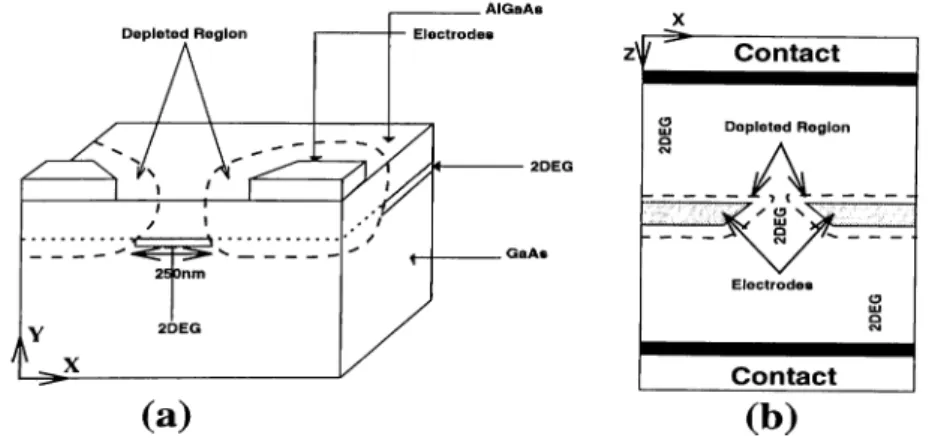
pioneering works have been reached by van Wees et ah'* as well as Whararn et al.,'' who were able to see quantum conductance phenomenon with cui error less than 5%. That has been a break-through in the field of ballistic transport in mesoscopic physics. The experimental set-up which introduced the quantization of conductance in 2D EG is shown in Figure 1.2. In this system, point contacts are made on high-mobility molecular-beam-epitaxy-grown GaAs/AlGaAs heterostructure. The 2DEG, which is formed at the interlace between GaAs and AlGaAs slabs has mobility ~ and density ~ 10^'^/m^ .so that the Fermi wave length ~ lOOA.
On the top of the heterostructure, a metal gate is made with cui opening ~ few \ p (Fermi wave length) and much smaller than /e(mean free electron path). The point contacts are defined by applying a negative voltage Vg to the gate. For smcill Vg, the 2DEG (formed at the interface between GaAs and AlGaAs) which is underneath the gate is depleted and the conduction is taking phice at the contact only with width w ~ opening of the gates; by further decreiising of
CHAPTER 1. IN T R O D U C T IO N
Figure 1.2: Schematic Diagram of 2DEG Quantum Point Contact, (a) lateral crossection view and (b) top view.
Fg, the depletion layer increases and the width of the point contacts is reduced griiducilly until it is pinched off completely. Therefore, with this novel device, we can vary the width of the QPC for a given device configuration by changing Vq only.
With this device, two terminal resistance of several point contacts as a function of gate voltcige was measured'*’® and in Figure 1..3 we show the experimental results of Vein Wees et ah'* after contact resistances are subtracted. It is clear from the graph that the conductance of the QPC as a function of F, changes in the form of a stair-case with steps of 2e^//i within a precision of few percent.
These experimental results have brought a new insight to the physics of QPC which was known as early as the mid 60’s; Sharvin^ has calculated the conductance of a point contact using Drude approximation and found it to depend on the Fermi energy of the system and its geometry through the relation
2e2 A G. = —
h Xf'F ( 1.1)
where /1 is the contact area for 3D point contacts and slit opening for 2D. Eventhough the results in Figure 1.3 are in agreement with the Sharvin’s approximation for conductivity; i.e, G ~ ro, the jumps in the conductivity are not consistent with the constant slope for the Gs versus to curve of Sharvin’s conductivity. In fact this main difference in conductivity between the
Figure 1.3: Conductivity v.s Gate voltage for 2D EG which shows clearly the conductivity quantization.Ref[4]
experimental results and the Gs is due to dimensional effects. In Sharvin’s study (and early approaches), point contacts scale length A/?, and as a result, qucintization effect due to the constriction width w is smeai'ed out mainly due to the tunneling phenomenon; therefore in early studies quantization effect was not taken into consideration. However, with these new experimental results, a. more detciiled solution need to be carried out to show the ciuantum size effects, and this was cleared up'*’® in terms of the subband formation which was explained earlier.'
In order to understand this phenomenon better, we consider the following simple derivation. At the interface between the two slabs GaAs and AlGaAs, the 2DEG is constrained to a certain well cilong the {x^y) direction due to the depletion generated by the negative gate voltage, but it is free to move along the channel (z) direction. Therefore we Ccin represent the potential confinement by
V ( x , y , z ) = 0 for 0 < X < Lx and 0 < y < Ly oo otherwise
(1.2)
The solution to this problem is quite simple and we can separate the wave function to lateral part (in the x and y direction) and longitudinal one (in the .2 direction).
CHAPTER 1. IN T R O D U C T IO N
and we will get energy eigenvalue
,, ,, n'^ki E — E%' x!
---2rn (1.3)
where is the propagation vector along the ^-axis.
On the (x^y) plane, we have approximated our potential as a quantum well with an infinite wall barrier and this would yield the vanishing of the wave function at the boundaries giving rise to only some possible eigenfunctions to the problem with eigenenergy spectrum
E.v,y = En,,n,j = ^ 0 ^ 0)
where Ux and iiy are quantum numbers describing eigenfunction solution cuid Lx and Ly cxre the width of the channel and accumulation layer respectively as shown in Figure 1.2.
We note here that Ly <C Fa,, therefore mciny eigenstates corresponding to different /7 values and Uy = 1 would have a lower energy eigenvalue compared to the state with n,j = 2; as a consequence, we can disregard the y dependence of the solution by assuming thcxt only nj, = 1 are the filled states of the system, so the energy of the system is
where the constant energy fi / (nyir/ LyY¡2m is taken to be zero by changing the reference of energy spectrum.
Connecting the chcxnnel to two reservoirs with Fermi energy Ep· 'At z = ±oo and keeping it at constant and small chemical potential difference A y , we can find the conductance of this QPC through the relation G = I / V . In order to find the current /, we will use the relation
/ = evpD(Ep)Ay (1.6)
where vp is the Fermi velocity, D(Ep) the density of states at Fermi level and A y is the chemical potential. For the multiple subbands Ccise, we will Imve
I = eJ2 v„JEF)D„JEF)Aft (1.7)
where is the subband index. Assuming no subband interaction occurring in such a system, the generalization of the one band system gives
\/2m D{E) =
v{E) =
I1E 2 '~2
Y (with spin degeneracy and positive A:,) E2
(1.8)
(1.9) VVe note here that we have taken only electrons in the energy range AV ¿uid Ep + AyU (only these ones contribute to the effective current) and with positive A;,, in the calculation of D{E) because the ones with negative Au do not enter the chiuinel and they do not yield any current contribution to the system. Therefore
/ = x :e ( £ :p - (1.10)
hm ■
where Ep — En^ = is the longitudinal energy of the electrons in band which has to be positive to be a current carrying state. Since J2nr ©(•¿'V “ -£'»,;) = N ^ totiil number of bcinds with energy E below Ep so
Thus 2c I = h V h V h V h (1.Ü ) (1.12) Obviously we can understand better the staircase structure shown in Figure 1.3. As the gate voltage is increased, the depletion layer decreases cillowing more stcites dipping below the Fermi energy and every state would contribute to 1 “quantum conductance” (2e^//i). Therefore, we can explain every step in conductivity graph of Figure 1.3 by dipping one more state below the Fermi level.
Eventhough this theoretical derivations made us understand better the experimental results, further investigations of the cipproxirnations need to be carried out to understand the applicability of the theory and this would include tests on the following parameters
CHAPTER 1. IN T R O D U C T IO N
• The potential profile, which is assumed to be a perfect qucuitum well ignoring ciny variations which may occur due to surface roughness.
• Contacts occur at the 2 = ±oo and this would prohibit any tunneling or reflections at the boundary edges of the channel.
• Band mixing is ignored and this is true only at T = OA' and at perfectly smooth surface.
The effect of the confining potentials has been the object of detailed ccdculations.“’“^'* In these calculations, it W cis shown tlmt for long constriction
(A. >> A/,'), the conductance is directly proportional to integer number of propagating modes or conductance channels cind increases with increasing width of constriction in steps of 2e^/h when a new channel opens up. Even in the case of constriction length ~ A/?, the conductance still show staircase structure with oscillatory behavior.'·^ However in the case of very short constrictions (A~ <C A/,·) where tunneling becomes important in such systems and the stair-case form is smeared out, and we cipproach Gh curve as —> 0.
Based on these theoretical studies, we can conclude that, the potential profile or surface roughness itself does not change the general feature of the G curve since ciny potential profile which yields quasi bound states give rise to such jumps in the conductivity whenever a new bound state dips below the I'ermi energy. However the length of the channel plays an important role in these calculations, since shorter constrictions cause more reflections of the eigenstates cit the boundaries of the channel and these would introduce oscillations on the pla.teaus^·'^ of conductivity and, for A^ ^ A/r, tunneling phenomenon becomes pronounced and stair-case structure starts to disappear reaching Sharvin curve for A- ~ 0.
Temperature dependence on conductivity in many subband system was studied throughly by M. Biittiker et a/.^*^and they found a genercilization of Landauer’s formula® at finite T. Another approach was used by Tekman and Ciraci,^·* who have used the variation of D(E) at finite T in equation 1.7, while calculating the current /, and they found that for very thin constrictions
(L.,; ~ 2Xp) where the energy difference between energy eigenvalues are quite large compared to the case of wide ojaenings, temperature effects a,re quite snicill up to T = 5 /f and they just diminish oscillations occurring at the plateaus. However, for the case of large openings (Lx ~ lOA;?), the inter subband mixing becomes very important and the stair-case structure disappears for T > 0 .6 /i. Within these theoretical calculations, based on free electron model and an approximate potential profile confinement, it is generally accepted that this model explains well the 2DEG experimental results, except for the resonance structure superposed on the plateaus which is due to reflections from the ends of the channel and was not detected experimentally.
Coming back to the work done by Gimzewski and Möller^ in which tunneling current exhibits a jump and saturates as the tip is brought closer to the sample at a certciin tip-sample separation distcince. If we use the results of this experiment and plot G versus tip displacement, a plateau would show up. Analysis has shown that the discontinuous jump is due to the adhesion of the tip to the sample, wliich happens when the tip-sample system is unstable at certain separation. In this case the tip elongates towards the sample and forms a mechanical contcict in the form of a neck as shown schematically by Gimzewski et al.A They have estimated the contact radius to be ~ \ p . Therefore, length in such systems is of
the order of \p^ and the observed trcuisport beyond the discontinuity in Figure 1.3 has to be associated with ballistic quantum transport. As a result it would l)e possible to generalize the theory applied to the 2DEG to this system. Garcia*' was the first one who pointed out that the point contact in STM is relat<xl to ballistic transport of electrons through QPC. Following these predictions, Lang*^ has simulated the point contact experiment by two jelliurn electrodes, one of them having an adsorbed Na atom on it cind thus representing a single atom tip. He found that the conductcuice saturates at a value of rße^lh and forms a plateau, where the Vcilue of 7] depends strongly on the identity of the material and it is only 0.4 for Na. Different approach was used by Ferrer et who have studied contact resistance of STM at a very small separation using tight- binding Hcimiltonian and Keldysh (non-equilibrium) Green’s function fornicdism
CHAPTER 1. IN T R O D U C T IO N
arid they have found that the conductivity saturates at close contact ~ 2. 5A. to a Vcilue ~ 2e^//г. In parallel with these two different approaches, Ciraci and Tekinan^° Imve studied the transition from tunneling regime to point contact in STM within Self-consistent-field (SCF) pseudopotential method and they found thcit the variation of G as a function of tip-sample separation is sample and tip specific. Moreover, they have explained the observed jumps of G by the irregulcir enlargement of the contact area. Nevertheless, we Ccin state that the step structure can also be revealed in 3T> QPC, which seems to be explained by using ballistic theory. In treating the experimental results of Gimzewski et al.,^ we should note that the diameter of the neck is ~ Xp] as it is already concluded in the theoretical s t u d i e s ,th a t we can not really expect shcirp qiuuitizcition in such experiments.
1.2
E x p e r im e n ts o n L o n g Q u a n tu m W ir e s
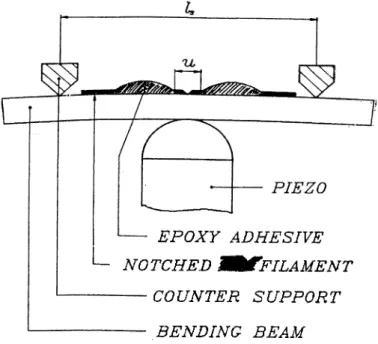
Ifecently, by pulling the tip after nanoindentation^^"^·^ or by using a mechcinically controllable break junction system (MCBJ)^'^“^^ long metal wires with diameters in the range of a few have been produced. As the crossection of the wire is rcxluced by stretching it continuously, the two-terminal conductcuice G Ims been measured. In Figure 1.4 we show the schematic description of a MCB.J ta.kcn from reference 25. Referring back to this figure, the sample in the shape of a metal filament is glued on a substrate (bending beam), then by bending the substrate in high vacuum, the filciment is broken. The electrodes, which are thus freshly exposed, are brought back into contact. The bending which is controlling the separation distance between the ends of the wire is controlled by tuning the piezo voltage Vp allowing fine adjustment of the separation between the electrodes. In the STM experiment, the tip is pushed into the surface beyond the separation distance at which the jump to QPC occurs cind then it is slowly retracted yielding to a long neck formation'^'* of~ 40A.
Eventhough the experimental set-up of the STM and MCBJ are different, the principle of neck formation is the same: stretching a iruiterial with a small contact
areci of ~ lOA cind measuring its two terminal conductance G. In fact these experiments have been done on a variety of rnatericils cUid here we will show some experimental results and make some comments on them.
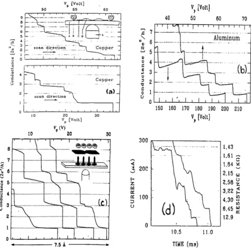
in Figure 1.5, we show some experimental results obtained from Cu, Al, Na cuid Au. The conductivity in the first three plots were measured by MCB.J while that of gold was measured with STM set up. From these plots, we Ccin recognize some interesting features occurring in the conductivity measurements which are absent in Figure 1.3 showing the quantization in 2D EG. The most important differences include
• STM and MCBJ give the same general graph features for the conductivity. • Results for Na (in Figure 1.5-c) show clearly that these experiments are
quite irreproducible apart from the last plateau which survives for a longer time interval compared to the other ones.
EPOXY ADHESIVE NOTCHED mm^FILAMENT
COUNTER SUPPORT BENDING BEAM
Figure 1.4: Schematic diagram for mechanically controllable break junction. Ref. [25]
CHAPTER L IN T R O D U C T IO N 11 V, [Volt] 10 20 30 40 [Volt] 50 60 70 Vp [Volt] 1.43 1,61 - t.04 2 2.15 u 2.58 ^ 3.22 Í ^.30^ 6,45 w w 12,9
Figure 1.5: Conductivity in metal neck structures, (a), (b) and (c) are measured with MCB.J set up for Cu, A1 and Na respectively at 1.3/F as a function of l'^,(piezo voltage), (d) is Au conductivity measurement with STM set up ci.s a function of time before the neck breaking.Ref[25,22,26]
• For G > 6Go {Go - ‘¿e^/h) plateau structure starts to smear out and we cire in fact very close to Sharvin case.
• Plateaus may hcive jumps of ~ Go or ~
2Go-• For A1 and Au (Figure 1.5-b,d), we can see some dipping phenomena in the conductivity measurement at the beginning of every lower plateau. • For the A1 wire, we can also observe a small increase in the conductivity
0) N V O a (d -4^ o 3 •d c! o u
1
1 ' 1
— —'—1
—^
X...
Platinum
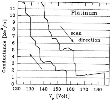
120 130 140 150 160 170 180 Vp [Volt]Figure 1.6: The conductance of a Pt junction at 1.3K as a function of Vp for two successive scans. In the first scan the transition was approached from the contact side whereas in the second scan the transition was aiDproached from the tunnel side.Ref[24]
Eventhough, metals are the best mciterials to be described by free electron model and as a result our generalization of quantization phenomenon would work best in such a system, we can see from the previous remarks that 3D QPC features differs from those of 2DEG. As a result simple generalization of the previous theory would most probably fail. In fact investigating other types of materials, such as transition metals (Pt) or semi-rnetals (Sb), shows well that this “quantization” phenomenon is quite fragile and it is too much material dependent. In Figure 1.6, we show the graph for Pt conductivity which exhibits the formation ol plateaus, but quite different from the ones shown previously. In this Figure, we also note that
The last plateau corresponds to a conductivity of
2Go-• The slope of the last plateau becomes much more pronounced relative to that of Al.
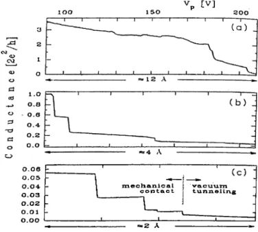
CHylPTER 1. IN T R O D U C T IO N 13 % [V ] 0.06 0.05 0.04 0.03 0 .0 2 0 . 0 1 0.00 z n e c h i a n i c a . 1 c o n t a c t ( c ) v a c u i a x T i tunneling -2 A
Figure 1.7: Three examples of conductance of a Sb contact at IMK as a function of Vp, with Vp increasing. The three curves are recorded for three different Vp sweeps. Curve (a) shows the behavior for a large decreasing contact size. In the mechanical contact regime shown in curve (c) as well as in curve (/;), the conductance is less than the quantum unit.Ref[27]
• Hystei'esis effect becomes much more inqaortant for this structure.
Concerning the results of semimetals, where we have taken Sb as an example, we show the variation of conductance in Figure 1.7. Here we can observe the following important feature
• “Quantization” phenomenon becomes nearly impossible to exphiin the plateaus which still occur but they exhibit jumps with a small traction of 2e^//г.
Within these new experimental results, it has become quite difficult to explain this “random” plateau formation with a simple generalizcition ol the theory applied to 2D EG. Hence, for the last three years the problem has been revisited with the hope of resolving this quantization phenomenon.
1.3
T h e o r ie s
It has l^een suggested that these plateaus occurring in the conductance in the QPC regime are due to discontinuous change of atomic structure/'^’'^^’^'^ and evei\y atom cit the narrowest part of the neck opens a channel when one of its states t„. is in common with the Fermi level. Even if e„, is above the E[,·^ ballistic transport may still occur because the state is broadened and becomes a resonance'^‘^ centered at
£ = Co. + A (1.13)
with FWHM r, and 1ms density
P a ( e ) = A / 7 r [ ( e - e „ - A ) ^ + F2 i - l (1.14)
The distribution Pa(c) may have a partial overlap with the Fermi level and hence the conductcince over this resonance may be smaller than Go- Therefore, the total conductivity ol the neck would be the sum of individual atom contributions which are at the neck. On the other hand, still there are some who believe that this sharp step structure indicates the unique transversal qucintization along the 3Z1 c o n s t r i c t i o n , a n d they cissurne that the energy states vary adiabaticcdly so that the channel mixing due to finite bias, temperature cuid saddle point potenticil is marginal. The height of each step is eqiml to 'u-multiplc of Go·, where n being the degeneracy of the corresponding state below Ep. In addition to this, marginal differences from “quantum” conduction could be well explained through scattering phenomenon due to potential variations at the neck. Until today, both views cire still a m atter of dispute between different groups^^ and the quantization of conductance in atomic wires is not completely resolved.
In order to understand better the quantization phenomenon, we hcwe decided to make a study on the atomic and electronic properties of these nanostructures. Firstly, we will treat our system with free electron model in the bcdlistic regime. In the next cha2Dter, we will show our conductance calculation for different neck profiles in order to grasp the effect of quantization phenomenon in small systems. Following this, we will make a detailed atomic structure analysis for
CHAPTER 1. IN T R O D U C T IO N 15
neck samples while pulling. Because in small systems such cis atomic scale wires, the mechanisms of deformation and hence propensity for the creation and propagation of dislocations is reduced.^ The structural changes occurring in such systems are quite different from the bulk material and for this reason we ha.ve rricide simulations with Molecular Dynamics^^(MDS) on small structures to understand structural deformation in them and attempted to investigate the control i^arameters including: pulling rate, temperature, crystal structure and interaction potential type. This study will be presented in chapter 3. In chapter 4 we will introduce Self-Consistent-Field (SCF) calculations for different neck scimples and infinite wires in order to understand the physical difference between the finite and infinite size nanostructures. Finally in the concluding section we address to the questions we raised while analyzing experimented results on the 3D QPC with the hope of providing better understanding.
B a llistic tra n sp o rt th ro u g h
ZD
Q P C
2.1
T h e o r y a n d g e n e r a l fo r m a lism
W(' have seen in Chapter 1 that in the 2 DEG, quantization plixinoinenoii of 2D QPC is clue to the quasi — ID nature of the system, and there were many theoretical studies devoted to explain this phenomenon. Now we would generalize the formalism'·^ which has been applied by Tekman and Ciraci.
In this ap2:)roach we will divide the space into three parts: 1) the left most and 2) right most parts are two semiinfinite jellium electrodes, so the Shrddinger ecpiation in this portion of space would simply give a free plane wave particle solution. 3) the centred part of the constriction which is characterized by a laterally confining potential, and as a result, the solution of the Shrodinger equation in this region are subband wave functions arising from the (]uantization of the transverse momentum. The separation of space into jellium electrodes and constriction can be represented by using profile cordinernent V{x,y ,z) defined Iry
V ( x , y , z ) = \(j),n{z) + VQx,y,z)]0{z)0{d- z) (2.1)
where 0 is the step function and d is the constriction length; here the potential is taken zero in the left most {z < 0) and right most > d) i-egions, while
CHAPTER 2. BALLISTIC T R A N SPO R T TH RO UG H W QPC 17
at the constriction (0 < ^ < d), the potential has two parts, the longitudinal part (Pmiz) (which contains the variation of minimum value of potential along the constriction) iind the confining part Vc{x,y,z) (which gives rise to subband structure). For a general constriction, it may not be obvious and may even not be unique to decompose the potential V {x ,y ,z) to this type of confining model, however, in necirly free electron a p p r o x i m a t i o n , t h e 3D potenticil of contact is obtained from SCF calculations and is parcirneterized
V{x, y, z; d) = </>„,,(z; d) + a{z] d){x^ + ?/^ (2.2) here X and y are transversal coordinates and is the longitudinal coordinate from left electrode towards the right electrode along the axis of contact; while d is the constriction length.
The hamiltonian lor the QPC is written as H =
2m* V^ + V{x,y,z) (2.3)
where m* is the effective mass^ of the electron propagating through the constriction and it is assumed to be isotropic. Therefore Shrodinger equation would have the form
rc æ h
2rn* dz^7 ^ + + ^o(x, y, z) ~) = 7í'0«,s(■г·, ?/, z) (2.4) where V|| = d^jdx^ + d^'/dy^, the term n corresponds to the subband wave function induced due to the confining potential V^(.'c, ?/, z) and the energy is assumed to be continuous due to the propagation along the ^ axis. We note here, that the solutions of Shrodinger equation are two-lbld degenerate; if i/>n,/i(.'fb ?/>-^') is a solution of eqiuition 2.4 with left current currying state, then Vhi,£;(·^)
also a solution and corresponds to the state which carries current in the opposite direction.
^In our calculations, we would use effective mass theory which treats the effect of the atoms |:)otential as renormalization of the free electron propagation energy. Our approximation is justified because our system size contains a large number of atomic cells and the external potential is slowly varying over atomic scale length.
The solution of the equation 2.4 is not alwciys possible, because generall}/ the pcirtial differential equation is not separable. Then we have to deal with solutions onl_y for very special potential confinements in section 2.2 and approximate solutions for a general confinement is applied in section 2..3. However, for the time being we would suppose the subband wave functions ?y, z) ¿ind ?/>„ ¿¿(x, ?/, z) are well known in the constriction and will find the conductance for such a system. Assuming that the subband wave functions in the constriction are known, the general solution of the Shrodinger equation in all space is found by matching these solutions with the phuie wave nature of the wave functions at the jellium electrodes (z < 0 cind z > d). To this end the following conditions have to be satisfied
• Continuity of the wave function and its derivative at the left boundary of the constriction (z = 0).
• Continuity of the wave function and its derivative at the right boundary of the constriction (z - d).
• Boundary condition at ^ = Too which define incoming and outgoing waves. Let us consider an incident plane wave from the left hand side of the constriction with wave vector Ki = k^„ is in the longitudinal direction. Aq,,, and ky^ are in the lateral direction, and its energy E = /¿^|/C:P/2?'n*. Since in this problem, we are assuming that the characteristic length of the constriction is smaller than the electron mean free path i.e the contact is ballistic; therelbre plane waves at the left most and right most sides and at the constriction have the same energy E and we will write the wave functions as
n
CHAPTER 2. BALLISTIC T R A N SPO R T TH RO UG H W QPC 19
where the first term of equation 2.5 corresponds to an incident phme wave and its reflection cit the left boundary of the constriction and this corresponds to the solution of the Shrodinger equation at the left most portion of space. The second term of our equation corresponds to the solution at the constriction and it is a combination of all the subband wave functions (left and right current carrying states). Finally the last term which corresponds to the solution cit the right most portion of space and it represents transmission through the constriction at .i' = d. Since the energy FJ in this system is conserved so kl(kx, ky) = 2rn*E/lP — k'f. — k^ and while taking the square root of this quantity, the imaginary part of k~(k.^, ky) is taken to be positive so that the function decays cis ^ ±oo in order to get physical solutions. Unknowns in the eqiuition 2.5 should be determined from the boundary conditions at ,? = 0 and z = d] continuity of the wave functions gives for = 0
= E y, + ^„,£,.(.'1·, y, 0) J (2.6)
n
a.iid for = d we get
2/, d) = {^I’u,e{x^ y, + ^n,£'(-U !/>
n
=
J
dk^dkyP^dk.Fy)d^ik,x^ikyy]:^^^(^f^^j^^^^ ^2.1) Along the X and y direction the wavefunction continuity is gruiranteed, since all subband wavefunction solutions in the constriction would satisfy this condition, 'riiis continuity of the wave function in the x and y direction guarantees the continuity of its derivative. However in the .ir direction we calcuhite the wave function derivative in order to match it at ^ = 0 and z = d and this would give l-v k ,, (.T,?/, z)l,=o = _ j dk jk yz k, { k ,, (A·,, k,,)= 5 ] + ?,г,£;(·г■, 2/, -^)|,=oA,, (2.8)
this for z = 0 cind for z = d we get
=
J
(2.9) liciving expressed the boundary conditions for such a system, the coeflicients Aj:^(k^.^ ky), Bj^.(kx,ky), and luive to be determined cis a function of the incident wave vector Ki and this is done by solving equcitions 2.6, 2.7, 2.8 and 2.9 simultaneously, and j^.{x,y, z) will be determined in ¿dl space. Eventhough those coeflicients can be determined exactly, the solution is not simple. We need to tcike the Fourier Transform (FT) of these equations in order to get rid of the X and y dependence in the final expression so that the manipulation of these equations will be ecisier; to do this we will define the 2D FT of a function f{ x,y ) as<ly) = ^ /_ " dxdye--’^^^e~^'>’^yfix, y) (2.10) taking the FT of equation 2.6 and 2.7 we get
27T [¿'((/^. - k^J)b{qy - ky,^) + Aj^^{q^,qy) =
qyi d” H.n,Ei(lxi %■> }
n
\Hn,E{qxi qyi d)0^^ j^, + rfri,/i'(<Z:i·) % 1 }(·^· ^ 0
n
where 11 and fl are used to denote the P'T of the subband wave function of ■tj> and ■(/». Now taking the FT of equations 2.8 cind 2.9 we get
27T [iKJiq.^ - k^„)8{qy - ky^) - ik^{qxiqy)Aj^^{q.^,qy) =
n
E { n i,E (i.. 9,. <*)».,,?, + K eUi·., <h„ <0 A„jr, }(2. 12)
n
where If' and If' are used to denote the subband wave function derivatives of (/>' and along the .2—direction. From the previous two equations, elimination of the reflection coefficient Aj^.{qx^qy) gives
CHAPTER 2. BALLISTIC TR A N SPO R T TH RO UG H 3D QPC 21
(ly)^^n,Ei(lx ·, (¡y·) 0) ([y^ n
~i~[kz{(lx^ qy)Hn,Ei(lx·, (Jy, 0) — q.y^ ())] |( 2. L3) and the elimination of transmission coefficient Bj^Xq^^qy) gives
Xv Qy)^^n,E((Ix'> Qy·) + zTI^^ qy^ n
+ [^’^(</x-5 <Zl/)ri7l,£'(</.r5 </y, iO ~ 0(2.14) Equation 2.13 and 2.14 have to be solved simultaneously to obtcun the coefficients 0^^ and f·-. where Ki is the incident plane wave vector. Here we note that equcition 2.13 stands for the transmission of incident plane wave into the subband states cit the enti’cince of constriction (z = 0), and equation 2.14 corresponds to the reflection of subband at the end of constriction (z = d). Therefore once the solution of Shrodinger equation (equation 2.4) in the constriction is determined and the snbband wave functions are known, the problem reduces to calculation of multiple reflections from the edges of the constriction, it is then a simple algebredc problem.
Assuirdng that these coefficients are determined, and 'if z) is calculated throughout the constriction, we will detenrdne the current passing cicross the constriction in order to find out the conductivity. In order to calculate the current, it is clecu· that calculating through any contact crossing the a.xis at .2 = z^, would yield the same result, since the current inside the system is conserved. To do this we choose (z < Zo < d), so that the final current expression consists of subband wave functions. The current passing through the QPC is related to tlie occupation of subbands as in the Landauer forrnula.^’^^
'I’he current due to incident waves ?/)« and with energy E can be written using the expectation value of the current operator
{'MM
=
J dxdy
[V
’*(a:,
y^x, y) -
C'(•'^b
'!j)'<hi-C
?/)] ^ (2.15)
^Here we note that we are using the sign * in order to denote the effective mass if it is a superscript of the character cind a complex conjugate for any other variable.
In our system we should take into account all contributions İroni all incoming states Hence,
J { E ) = 2 e I y, y, ~
Where J(E) corresponds to the electric current due to the states with energy E. Here we have introduced the factor e in order to convert the probability current into the electriccd current. The iirefactor 2 takes care of spin degeneracy and 1/ ( 27t)·^ is the density of states in the 3 D /’f —space, S function selects the states
which have energy E and the step function 0 selects electrons with positive so that only electrons entering the channel are taken into account. In order to evaluate J{E) we will initially calculate at an arbitrary point
in the constriction.
7H,n
- [ i ’n,]sU=^oK,P, + + Au,E\z^^,Arn,Kj
(2.17) In this equation, lor clarity we have dropped the {x,y,z) factor which is iu tlie front of the subband wave functions; further manipulation of this equation yields
m,n _ _/ _/ + ’/ ’n.B I - ^ = - ' o ' 0 m , 7 J I € ) „ i , / q } ( 2 . 1 8 ) Finally we obtain e 1 dky^ j ( E ) = J _ / ttIi 2tt Jkl^-\rkl^<K% Am
I
[ / d.xY/?/V7*,fc.L.=,,y0'„,y^|,r=.r,J0,„./q 7) J. 77.CHAPTER 2. BALLISTIC TR A N SPO R T TH RO UG H :W QPC 23
+A*,7í*.[/ í¿-cí¿yK3'l-^=^oV4,¿’L-..o]0„,,,,e, (2.19)
Here wc have introduced a new variable K'^ = E 2m*fh^, and the f corresponds to the 2D integration in the A:—space such that + < Kp; with the constraint k'i + ky^ + k't^^ = Kp; has to be satisfied while evakuiting the previous integration. Now we will assume that our constriction is connected to two jellium electrodes at ,2 = ±oo and the electro-chemical potentials of these two reservoirs iire kept constant so that there is an infinitesimal difference A/j, - ¡ij^ — /.ir > 0 between the electro-chemical potential of the left hand side and the right hand side of the reservoirs. In this circuit current would flow from the left reservoir to the right one and vice versa and in experiment we would measure only the effective one. I'o rnecisure the current due to one electrode, we should integrate J{E) factored l)y D(E), which is the electron occupancy with energy E, over all the energy range. In our calculation we will take D{E) = fpT){E) which is the Fermi-Dirac distribution at T = OK so that it corresponds to step function; therefore the current flowing through the circuit is
i'HL I = J J{E)dE - J{E)dE C HR — / J{E)dE ■= {¡XL — ER)d{pR) I/O. = A¡.íJ { Ef) — e VJ { Ep ) (where {/xl - ftn) -> 0)
(fXfi = Ef, Fermi energyX2.20) ff'he conductance is
G = ^ = eJ{EF) (2.21)
By determining J{E) from equation 2.19, we obtain directly the conductance in the constriction after multiplying by e. In the next section, we will solve this problem lor a uniform constriction, followed by an approximate solution for a more general potential type in section 2.4.
2 .2
C y lin d r ic a l In fin ite W ell C o n fin e m e n t
2.2.1
Form alism
In this section vve will assume that the confining potential is indepenclcnt from .r. As a result 4>m{^) — 0 ^.nd Vc(x·, y, z) = K.(.c, y). Furthermore we assume that this |)otential is oidy radial. We first treat the infinite wall cylindrical confinement potential in this section. Then we consider parabolic one. Eventhough these profiles oversimplify the real potential, we believe that some insight of the problem could still be grasped. Our potential confinement would have the form
where V{p) = (2.22) (2.23) V{r) = 0{z)e{d - z)V{p) 0 p < 10 oo otherwise
Wh('re (/) and describe cylindrical coordinate system. This describes an infinite cylindriccil wall potential with uniform crossection, in the regions 0 < .i < d and 0 otherwise. Due to p dependence of the potential, we will write Slirödinger ecpiation 2.4 in cylindrical coordinate system a.nd it becomes
IP
where
72 I d d . I d'^
(2.25) p dp' dp fP d(j)'^
in cylindrical coordiiicite system; this equation is separtible and we can write
(2.27) wliere the lateral wave function satisfies the differential equation
rP
[ - ^ V j j + Vc(p)]^nip,(/^) = en^n{p,(f>)
with subband energy e„ and propagation vector along the ^-ax is 7,,, satislyii (2.28) / 2??r* , s
In = \ l —r - c ^ - ^n) h
CHAPTER 2. BALLISTIC T R A N SPO RT THRO UG H W QPC 25
where the root with positive imaginary value is taken.
Since the potential in equation 2.27, has only p dependence, we can separate our equation into radial and rotational parts and we can rrurke the Ibllowing transformation: ^ n i p . f ) — Rnt{p)P‘'^ where the radial part R„,t satisfies
r IP 1 d cl IPP 1 ^ ,
+ (2. 29)
with boundary condition Rni{w) = 0
Manipulating this equation with transforrncition p = au we get the following form (2.30)
{“¿“I;
“
2rncP where ■ ■ -p — tni = 1 ¿III cl Ri l l w 0d'his represents Bessel’s equation of the first kind and its solution J/(u) is straight forwa.rd , however, the vanishing of the function at the boundary yields to only some possible eigenstate solutions
and Rniip) = AniJliUril—) to IP (2.31) ^nl (2.32) 2mw^
Hence the lateral wave functions have the form ^ni{pA) = AraJi{rcnA^
where / is the order of the Bessel function and Uni its zero, while the term Ant corresponds to the normalization constant solved through the equa,tion
pw r2'7T
/ pdp d(/)^niip,<l>)K'i'(py(l>) = ^nn'dii'
Jo Jo
By solving this equation to find Ant, we get the final form of the lateral wa.ve function as
^nl{p, (/)) =
From equation 2.28 the longitudinal wave vector have the forr:n:n 2772 thus Jrd kp
\
_ {Unll^Tty { w I X p f (2..35)In the previous section we have shown how the solution of such a system is manipulated by taking the FT in the x and y directions, so now we will calculate this in cylindrical coordiricite system using
1 '(«) = ^ / n? )dp (2,:)6) a .n d ¿TV Jo Jo \ 10/ îJliKw) A — e - ' S '---!---j . 1 - f ^ V \ w»l / (2.37)
We note here thcit in this section we are using k = {k.,0^) instead of {qx.qy) as
the FT basis. We will write again equations 2.13 and 2.14 which now have much simpler form
2'K‘2,k,^/{K — Ko) — { [ ^ ’^ ( ^ ) T T [ ^ z ( ^ ) ~ 7n/]'^ n;,r-l} ) ( 2 . 3 8 )
a .n d
2: { i f e ( K ) - + [ U P + 7 n , l e - " “ " ' l A „ , g } = 0 ( 2 , : ! 9 )
nl
In order to solve such a system we will multiply every equation ( 2.38 and 2.39 ) l)y <[>*.;/(/i) and integrate over all k values, while using the orthogonality relation of the lateriil wave functions and thus its FT. The resulting equations are
27r7.2A.’2,j^,i'/'(^o) ~ ^ ) [2 { E n ' l ' ‘,nl T ' J n / n n ' ^ l l ' } O jil T 2 { E n ' l ' ; n l ' J n / n n ' ^ l l ' } A,,,;] nl
CHAPTER 2. BALLISTIC T R A N SPO R T TH RO UG H 3D QPC 27
and
'y ^ ' J n l ^ n n 'C E ) n l p t { R n ' l ' ; n l d“ 'y n l^n n '^tt'} (' A,(;J = 0
nl
(2.41) Here 6nn' is the Kronecker delta, and the matrix element Kn't'-,ni is delined through the relation
Rn’l'-,nl =
j
„,(/7)D(/c)$„/;/,„;(k) (2.42) Now we Ccin rewrite equation.s 2.40 cuid 2.41 in a matrix form .so that we can drop oil' our summation terms and we would obtain27Ti2k,^^HKo) = t { k + f )0 + i { k - f )À (2.43) and
i { k - f )D^''‘^0 + i { k + f )e~‘^''^A = 0 (2.44) Hei'<' 0 and À correspond to the column vectors of the coefficients of tlie suirband wave functions with right and left going probability currents, respectively. <I> is the row vector of the transverse FT of the latercil wave functions. F is a diagonal matrix of propagation constant vectors corresponding to every eigen state, and k is the longitudinal momentum matrix.
Now equations 2.43 and 2.44 correspond to the boundary conditions a.t = 0 and = d respectively and they can be easily solved to lind out the subband coefficients A =
C^kk + iT ^ik
0 = 2T r n - { k + r ) ~ k k - r ) ( . ~ l 2 - 1 (2.45) 2 k , j k + ! ' ) - ' (2.46) In order to find current J{Ef) we refer back to equations 2.18 and 2.19 and we would get(ir|j|^ ) = 0 _ ¿AU^'A + ¿Aff'0 - г h
where T/i and F/ cire the real and imaginary rncitrices of the matrix F, respectively. From these results, equation 2.19 would give us much simpler form by replacing the cartesian coordinate system with cylindrical one cuid by using the fact tha.t equations are independent of 0^. Thus
2e 1 kcIk.
= T T . C + 2a ”> ie 'b A ]}
To further simplify we introduce the following nicitrices
n = 2 I
-A = ~r = {¡< + T ) - U r - f < ) (K + F)n -1 (2.48) (2.49) (2.50) (2.51) As a result, the conductance becomes2 e ^ f K p k,cIk . o . . r - . .
C\7 = 4 - 2TT / ' 7^ ^ :^ (/i)]$ (/c )[fiT H n -A 'fV iA ]$ + (/i) + 2QTn4)(K)[n\l\A]#t(K) z t ^
h/ Jo L
(2.52)
In tins eciuation only and # are function of k. Since k.;{K) is real for |/i| < Kp··, one gets, by using equcvtion 2.42,
'SteK = 2nJ^ /cd/i$^(/c)A:;j(/i)l>(/v) (2.53) Finally the conductance formula reduces to the form
2fi2 G = — tr
a n ^ f/in - A^ffiA + 2i>?7i(lVr/A) K (2.54) In this equation there are 3 terms contributing to the conductivity; the first and the second term cori'espond to right and left going wa.ves in the constriction, respectively. Resonance effect may appear in the system due to their relative phase difference. The third term, corresponds to evanescent states^ in the constriction.^^ For finite length constrictions, where tunneling phenomenon becomes important, this last term becomes important since it yields deviations from sharp steps structure.
^y\ssuniing perfect conductivity in the constriction; i.e, as d oo, such states f with Cni > Ef ) do not contribute to conductivity
CHAPTER 2. BALLISTIC T R A N SPO R T T H R O U G H 3D QPC 29
Before introducing our results, we would like to bring the following issue to the reader cittention: Since we are measuring conductivity for a ballistic system (no scattering is occurring), shouldn’t we get G oo?
In fact this question has been addressed previously, while calculating the conductivity of 2DEG QPC. Imry^^ has showed that the finite resistance obtained in such formúlele was the contact resistance and did not correspond to the constriction resistance which has to be zero. This type of resistance mea.surement is known as two probe measurement and it has been thought that the resistance of ci perfect conductor vanishes for /our-probe measurement, where one uses different probes for the current and voltage measurements which are very weakly coupled to the device. In experimental set up, however, the lithographic shape of the current and voltage probes are the same in the ¿two-probe as well as the four-prohe measurements. For this reason it becomes impossible to assume weak coupling for the voltage probes. In lact Biittiker^*^’^^ has considered the coherent device consisting of the probes in addition to the loops or wire and calculated the scattering matrix for this device, where all probes are assumed to be connected to reservoirs at equilibrium. He has found tlicit the resistance VfUiishes ordy for very weak coupliiig(/o'ur'-probe iTiecisurernent) which does not correspond to the experimental conditions. As a result we have used ¿rwo-probe measurement to calculate the conductivity in our theoreticcil study.
2 .2 .2
R e su lts
In equation 2.54 we have obtained the hnal result of the conductivity for a perfectly cylindrical potential, by the integrcition over cill the incident wave vectors in ec[uation 2.52. The result is expressed only in terms of matrices. However, here we would like to mention an important difference between our results and experiments in which conductivity is measured. In the latter, G is measured as a function of Vp (piezo voltage) or the neck length, whereas in the former, it is calculated as a function of the electron density (or equivalently Xp) iind the area of the constriction A. Here we note that this mciin difference in conductivity
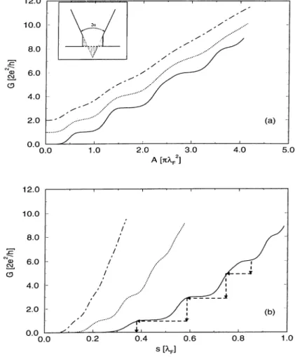
inecisurement is clue to the fcxct that in the thceoretical studies, Cinergy bands l)elow the Fermi level (which defines our contact area) are the criteria lor the conductivity; however, experimentally, it is not possible to measure the contact area at the constriction. On the other hand, there were attempts to estimate the confining potential profile (which would give the contact area) as a function of pulling using sirnuhvtions with molecular dynamics,^® but these profiles are not uiuversal because they are obtained by empirical potential, and depend on initial structure configuration cincl stretch speed . It is, therefore, difficult to find out the correct potential profile confinement. Nevertheless, our SCF calculations as well as others’, h a v e shown that parabolic j^otential confinement works well for one atom contact and infinite wall cylindrical potential parameterization is good for many atom point contact and this has motivated us to use tliem.
As shown in the ¡previous section, we have to calculate the propagation matrix F given by F„;,„'/' - and we should evaluate numerically the longitudinal matrix K given in equation 2.42 with the wave functions described by equation 2.37. An important point that is worth mentioning is that tlie off- diagonal elements of K are very small compared to the diagonal elements. For the infinite wall confinement, they deviate from zero and they become appreciable only when the energy of the subband dips below the Fermi level. 'J’hus I’ and K can be represented by finite dimensions, since in our calculations, we are interested at most upto the 5^^ energy subband. As a result, contributions from higher energy subbands would be small and we have noticed that 12x 12 matrices give results with convergence less thcin 2%, and in all our ccilculations we have used 20 subbands to get better convergence.
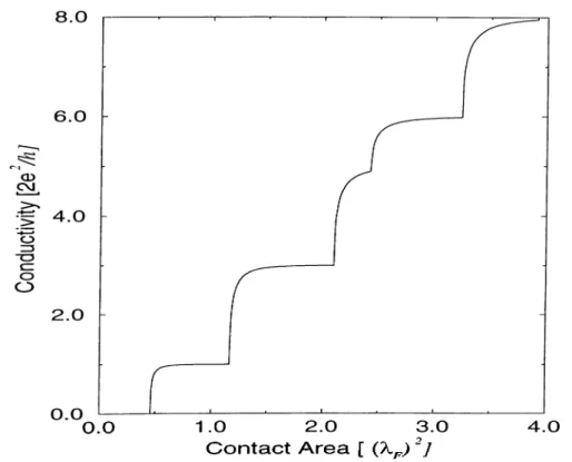
Initially, we will investigate the case of a semiinfinite constriction. In such a system contributions from the left going and evanescent states should he eliminated cind, hence equation 2.54 becomes
G = ‘^ t r j 4([A + + f]" '^ e (A 0 (2.55) In Figure 2.1, we show the results for a perfect semiinfinite constriction, in which approximate quantization of conductcince is apparent. This point is (piite
CHAPTER 2. BALLISTIC T R A N SPO R T T H R O U G H ‘W QPC 31
C o n t a c t A r e a [ “7
Figure 2.1: Conductance vs contact area due to trcUismission into seniiinfinite uniform constriction with cylindrical potential confinement
understandable, since ~ 7„n, so that the trace in equation 2.55 approaches to iVp. Now if we consider incidence from the constriction, the reflection amplitudes are given by equation 2.51. Here one Ccin directly use conventional Landauer’s formula^ in the channel cind we get
2e^ r
Gl = — |yV„ - (2.56)
where the first term is just the number of occupied subbands Np in the constriction and gives the incident waves. The second term is the contribution of the reflected waves, flere we note that G = Gl as a result of time-reversal
symmetry.
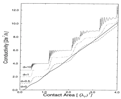
After examining the the semiinfinite constriction case, we will locus on the finite length channels, here we will solve equation 2.54 completely to find the conductivity. The results of our calculations lor finite length constriction are illustrated in Figure 2.2.
Figure 2.2: Conductance versus contact area due to trcuismission into a finite length uniform constriction with cylindrical potential confinement. The length of the constriction d is in units of Ai7.The grciphs have been shifted lor clarity.
The zero-length QPC was studied earlier.*^ Comparing the result obtained by using this formalism with Sharvin’s calculations,® we observe a great resemblance l·)(ítween them. The shcirp quantum steps have disappeared and there is n linear relation between the conductivity and the contact area as predicted previously by Sharvin. The washing of the quantum stej^s is not surprising, since as d 0 the probability of tunneling becomes apprecicible and this phenomenon dominates the conductivity. However, we can see in Figure 2.2 some deviations from Sharvin’s calculations; it is obvious that the “sti'ciight line” does not pciss through the origin and it exhibits some weak oscillations. The shift of the “straight tine” towards a larger contact area (A) value can be understood in terms of Heisenberg uncertainty relation. ApApp > fr, therefore as Ap —>· 0 the transverse momentum App —>■ + 00. Since the largest possible transverse momentum is hkp·, if pA:y,’ < 1 (or /l [A^] < 0.08) transport is suppressed to yield zero conductance as one notices
CHAPTER 2. BALLISTIC T R A N SPO R T T H R O U G H 3D QPC 33
in our graph. The weak oscillations, on the other hand, rruiy be thought as being the precursors to quantized conductance. For e„/ > Ep the transport is via tuuueliiig cind the conductance increases exponentially; when this subband dips in the Fermi level, the iiciture of transport changes to ballistic transport, and the inaxiiTium conductance for the subband is limited by the quantum of conductance {rn2cP/h where rn is the degeneracy of the state). Therelbre the conductance due to this single subband saturates leciding to the Ibrmation of weak shoulder like features as it is shown in our graph.
As the length of the constriction increases, tunneling contribution decreases and step structure of the conductivity starts to appear. The aforementioned weak oscillations superposed on the classical Sharvin conductance, evolve to form quantized platecius for d > Xp/2. This quantization phenomenon gets better with increasing d and they occur at multiples of 2e^//i with a step jump of one or ituo quantum steps corresponding to the degeneracy of the wave function in the cylindrical coordiimte system. It should be noted that these quantized steps do not represent the real experimental results represented in Figures 1.5, 1.6 and 1.7. In the experiments the plateaus are sharp cind they do not display the same degeneracy, while in the theoretical calculations the conductcmce displays oscillations below the quantized values which increase for larger constriction lengths (d) and subbands with smaller energy eigenstates. These oscillations are due to resonances caused by the interface of right and left going wavefunctions in the constriction. To analyze these resonances, we examine equation 2.50. The matrix exp[iVd] consists of pure phases for occupied subbcuids and varying the contact area [A) (i.e varying F), these phases change as well, and this yield an interfa.ee between the first and second term in the brackets in equation 2.54. After understanding the origin of these resonances, we won’t study this lurther. 4’he subject of resonance was taken into consideration throughly in previous s t u d i e s . N e x t we will generalize our formalism to a much more complicated potential profile in order to represent the experimental confinement better.
![Figure 1.1: Tunneling current versus distance z for a clean iridium tip and polycrystalline Ag surface: (a) approach (Vt = 20mU), (b) approach and retraction {Vt — — 2mU).[Ref.3]](https://thumb-eu.123doks.com/thumbv2/9libnet/5687779.114781/15.963.294.669.240.582/figure-tunneling-distance-polycrystalline-surface-approach-approach-retraction.webp)
![Figure 1.3: Conductivity v.s Gate voltage for 2D EG which shows clearly the conductivity quantization.Ref[4]](https://thumb-eu.123doks.com/thumbv2/9libnet/5687779.114781/17.963.316.651.235.536/figure-conductivity-gate-voltage-shows-clearly-conductivity-quantization.webp)