Parallel sparse matrix vector multiplication techniques for shared memory architectures

(1)

PARALLEL SPARSE MATRIX VECTOR

MULTIPLICATION TECHNIQUES FOR

SHARED MEMORY ARCHITECTURES

a thesis

submitted to the department of computer engineering

and the graduate school of engineering and science

of bilkent university

in partial fulfillment of the requirements

for the degree of

master of science

By

Mehmet Ba¸saran

September, 2014

(2)

I certify that I have read this thesis and that in my opinion it is fully adequate, in scope and in quality, as a thesis for the degree of Master of Science.

Prof. Dr. Cevdet Aykanat(Advisor)

Assist. Prof. Dr. Can Alkan

Assist. Prof. Dr. Kayhan ˙Imre

Approved for the Graduate School of Engineering and Science:

Prof. Dr. Levent Onural Director of the Graduate School

(3)

ABSTRACT

PARALLEL SPARSE MATRIX VECTOR

MULTIPLICATION TECHNIQUES FOR SHARED

MEMORY ARCHITECTURES

Mehmet Ba¸saran

M.S. in Computer Engineering Supervisor: Prof. Dr. Cevdet Aykanat

September, 2014

SpMxV (Sparse matrix vector multiplication) is a kernel operation in linear solvers in which a sparse matrix is multiplied with a dense vector repeatedly. Due to random memory access patterns exhibited by SpMxV operation, hard-ware components such as prefetchers, CPU caches, and built in SIMD units are under-utilized. Consequently, limiting parallelization eﬃcieny. In this study we developed;

• an adaptive runtime scheduling and load balancing algorithms for shared memory systems,

• a hybrid storage format to help eﬀectively vectorize sub-matrices, • an algorithm to extract proposed hybrid sub-matrix storage format. Implemented techniques are designed to be used by both hypergraph parti-tioning powered and spontaneous SpMxV operations. Tests are carried out on Knights Corner (KNC) coprocessor which is an x86 based many-core architecture employing NoC (network on chip) communication subsystem. However, proposed techniques can also be implemented for GPUs (graphical processing units).

Keywords: SpMxV, parallelization, KNC, Intel Xeon Phi, many-core, GPU, vec-torization, SIMD, adaptive scheduling and load balancing, Work stealing, Dis-tributed Systems, Data Locality.

(4)

¨

OZET

PAYLAS

¸IMLI HAFIZA S˙ISTEMLER˙I ˙IC

¸ ˙IN PARALEL

SEYREK MATR˙IS - D˙IZ˙I C

¸ ARP˙IM TEKN˙IKLER˙I

Mehmet Ba¸saran

Bilgisayar Mühendisli˘gi, Yüksek Lisans Tez Yöneticisi: Prof. Dr. Cevdet Aykanat

Eyl¨ul, 2014

Seyrek matris dizi ¸carpımı, denklem ¸cözücülerde kullanılan anahtar i¸slemdir. Seyrek matrix tarafından yapılan düzensiz hafıza eri¸simleri nedeniyle, buyruk ¨

on yükleyicisi, i¸slemci ön belle˘gi ve dizi buyrukları gibi bir ¸cok donanım etkili bir ¸sekilde kullanılamamaktadır. Buda paralel verimlili˘gin dü¸smesine neden olur. Bu ¸calı¸smada, payla¸sımlı hafıza sistemlerinde kullanılmak üzere,

• ¨O˘grenme yetisine sahip planlayıcı ve y¨uk dengeleyici algoritmalar,

• Dizi buyruklarını etkili bir ¸sekilde kullanmaya olanak sa˘glayan melez bir seyrek veri yapısı ve

• Bu veri yapısını olu¸sturmada kullanılan bir algoritma geli¸stirilmi¸stir.

Bu al¸smada belirtilen teknikler, hem ön yapılandırmalı hemde direkt olarak seyrek matrix-dizi ¸carpımında kullanılabilir. Testler Intel tarafından üretilen Xeon Phi adlı, x86 tabanlı ¸cekirdeklere ve bu ¸cekirdekleri birbirine ba˘glayan halka a˘g protokolüne sahip, yardımcı kartlar üzerinde yapılmı¸s tır. Önerilen teknikler ekran kartlarında da kullanılabilir.

Anahtar sözcükler : Seyrek matris-dizi ¸carpımı, KNC, Intel Xeon Phi, ¸cok ¸cekirdekli ilemciler, vektörizasyon, SIMD, ö˘grenebilen planlayıcı ve y¨k denge-leyiciler, i ¸calma, da˘gıtık sistemler, veri yerelli˘gi.

(5)

Acknowledgement

(6)

List of Figures

2.1 Sample matrix in 2D array representation. . . 9

2.2 CSR representation of SpM in figure 2.1. . . 10

2.3 Matrix rows are sorted by their non-zero count in descending order. 10 2.4 All non-zeros are shifted to left. . . 11

2.5 JDS representation of SpM in Figure 2.1. . . 11

2.6 Rowwise 1-D Block Partitioning algorithm for 4 PEs. . . 13

2.7 Columnwise 1-D Block Partitioning algorithm for 4 PEs. . . 14

2.8 2-D Block Partitioning algorithm for 16 PEs. . . 14

2.9 Column-net interpretation incurs vertical border. . . 16

2.10 Row-net interpretation incurs horizontal border. . . 17 2.11 A SpM is recursively reordered and divided into four parts using

column-net recursive bipartitioning scheme. And sub-matrix to PE assignment is done using rowwise 1-D partitioning algorithm. 18 2.12 An SpM is recursively reordered and divided into 4 parts using

row-net recursive bipartitioning scheme. Sub-matrix to processor assignment is done by using columnwise 1-D partitioning algorithm. 18

(11)

LIST OF FIGURES xi

2.13 High level view of on-die interconnect on Xeon Phi Coprocessor cards. TD (tag directory), MC (Memory Channel), L2 (Level 2 Cache), L1-d (Level 1 Data Cache), L1-i (Level 1 Instruction

Cache), HWP (hardware prefetcher). . . 21

2.14 Compact thread aﬃnity control. . . 24

2.15 Scatter thread aﬃnity control. . . 25

2.16 Balanced thread aﬃnity control. . . 25

3.1 Sample bipartitioning tree for column-net interpretation using CSR/JDS schemes on 5 EXs. . . 30

3.2 Sample matrix ordered by column-net model using rowwise 1-D partitioning algorithm for task to PE assignment. There are 5 EXs and collective reads on X vector by tasks are pointed out by density of portions’ color. . . 31

3.3 Bipartitioning tree for 2 blocks. . . 33

3.4 Sample matrix ordered by column-net model using rowwise 1-D partitioning using scatter distribution method. Collective reads by task on X vector are shown by the density of potions’ color. . . 33

3.5 Static routine sub-matrix distribution among 5 execution contexts. 34 3.6 Global queue and the order in which sub-matrices line up. . . 36

3.7 Ring work stealing scheme making eﬃcient use of bidirectional communication ring for 60 PEs. . . 37

3.8 Tree work stealing scheme in action. . . 38

4.1 Task decomposition for CSR format. . . 43

(12)

LIST OF FIGURES xii

4.3 Constraint violation in LBA is described. . . 55 4.4 LBA in action. . . 56 4.5 Sample output for CSR implementation of LBA. . . 59 4.6 Possible improvement for hybrid JDS-CSR format to avoid extra

prefetch issues. . . 60

5.1 Comparison of JDS-heavy CSR and CSR-heavy JDS in certain senarios. Hybrid format doesn’t necessarily contain both JDS and CSR everytime. In this case, cost of JDS and CSR are same. Therefore, one of them is chosen depending on the implementaion. 92 5.2 Comparison of JDS-heavy CSR and CSR-heavy JDS in certain

senarios. Here, at certain points costs are the same. Depending on version of LBA, one of them will be chosen. . . 92

(13)

List of Tables

2.1 Properties of Atmosmodd, it holds only 7 times the memory space of a dense vector with same column count. . . 8

4.1 Stats of choosen data sub-set. Row & column count, NNZ, and max-avg-min NNZ per row/column are given. . . 41 4.2 Eﬀect of discarding permutation array from JDS format. Results

are measured in GFlops and belong to single precision spontaneous static routine with 32KB sub-matrix sizes. Gains are substantial for matrices that are eﬃciently vectorizable. . . 46 4.3 Row & Column count, NNZ, and max, avg, min NNZ per

row/column are given for as-Skitter and packing-500x100x100-b050. 49 4.4 Time measured (in seconds) for 100 SpMxV operations performed

using as-Skitter and packing-500x100x100-b050 with Static and DWS routines both ’sp’ (spontaneous) and ’hp’ (hypergraph) modes. ’spc’ stands for spontaneous mode partition count while ’hpc’ for hypergraph mode patition count. In third row, how many times faster packing-500x100x100-b050 executes compared to as-Skitter is shown. (A hybrid storage format, proposed later in this chapter, is used to take these runs). . . 49

(14)

LIST OF TABLES xiv

4.5 Storage format performance (measured in GFLOPs) comparison for single precision SpMxV. For CSR format, the routine that per-forms best is chosen to include OpenMP Dynamic Loop implemen-tation. For JDS and CSR formats, results belong to DWS routine. 53 4.6 Hypergraph partitioning eﬀect is observed on diﬀerent schedulers.

’sp’ stands for spontanenous mode, while ’hp’ for hypergraph par-titioning mode. ’su’ is the speed up of hypergraph parpar-titioning based sequential routine over spontaneous sequential run. Out of 3 tree work stealing routines, only chunk distribution method is tested. Results are presented in GFlops. . . 63

5.1 CPU and memory specifications of Xeon Phi model used in tests. 65 5.2 Cache specifications of Xeon Phi model used in tests. . . 65 5.3 CPU and memory specifications of Xeon model used in tests. . . . 66 5.4 For all the SpMs used to test proposed routines, row & column

count, NNZ, min/avg/max NNZ per row/col, and their matrix structures are grouped by their problem types. . . 67 5.5 Performance is measured in GFlops and compared between MKL

and default DWS (DWS-RING) routine. ’spc’ stands for spon-taneous mode partition (/ sub-matrix) count, while ’hppc’ for hypergraph-partitioning mode partition count. ’su’ is speed up of hypergraph-partitioning use over spontanenous use while run-ning sequential routine. If, for a matrix, in spontaneous mode, DWS routine performs worse than MKL in either single or double precision versions, that matrix’s row is highlighted in red, statistics for problem groups are highlighted in blue, and overall statistics in green. . . 77

(15)

LIST OF TABLES xv

5.6 Diﬀerent variants of LBA are compared. Results are taken from single precision Static routine. Performance and measured in GFlops. Partition size is 32KB. . . 93

(16)

List of Algorithms

4.1 General template of application behaviour. . . 42

4.2 Kernel function for CSR format. . . 44

4.3 Kernel function for JDS format. . . 45

4.4 Kernel function for hybird JDS-CSR format. . . 52

4.5 Hybird JDS-CSR sub-matrix extraction. . . 54

4.6 JDS implementation of LBA to find the optimum cut for infinite vector unit length. . . 57

4.7 CSR implementation of LBA to find the optimum cut for infinite vector unit length. . . 58

(17)

Chapter 1 Introduction

1.1 Preliminary

Advancements in manufacturing technology made it possible to fit billions of transistors in a single processor. At the time of this writing, a 60+ core Xeon Phi coprocessor card has 5 billion transistor count. For a processor, higher transistor count means more computational power. But unfortunately, more computational power doesn’t necessarily result in better performance. Since computations are carried out on data, processor has to keep data blocks nearby or bring it from memory / disk when needed.

Increase in clock frequency implies an increase in data transfer penalty as well. In current era, the time it takes to transfer data blocks from memory dominates the time it takes to for processors to perform calculations on those data blocks. Because of the latency caused by transfer, processors has to be stalled frequently. Fortunately, most applications do not make entirely idenependent memory accesses. In general, memory access patterns express some degree of locality (classified under either temporal or spatial) [2]. Therefore CPU caches along with prefetchers are introduced in an eﬀort to keep data nearby for certain senarios. Substantially reducing average time to access memory.

(18)

On the other hand, sequential execution model reaching a point of diminish-ing returns, paved the way for parallel programmdiminish-ing paradigm. With this new paradigm, problems are expressed in terms of smaller sub-problems which are solved simultaneously. The process of dividing a workload into smaller chunks is called task decomposition. Task decomposition takes several metrics into account, such as load balance, data locality, and communication overhead.

Due to certain applications expressing definitive characteristics (such as pre-dictable access patterns, being embarassingly parallel...), specialized hardware structures are developed. In particular, vector extensions such as SSE (Stream-ing SIMD extensions), operates on chunks of data instead of individual elements in an eﬀort to improve performance. This is referred as SIMD (single instruction multiple data) in Flynn’s taxonomy [19, 20].

In this context, scalability of an application is measured by simultaneously running threads at its peak performance. Increasing thread count further after this point reduces overall performance which is measured in GigaFLOPs (one billion floating point operations per second). Scalability depends on application itself and measured on the hardware it’s running on. Therefore, eﬀectively using;

• prefetchers and CPU cache to hide latency,

• task decomposition to improve load balance, data locality, and to relax communication overhead, and

• hardware components built in for specific use, increases the scalability of parallel applications.

1.2 Problem Definition

In computer science alone, linear solvers are used in various, seemingly irrelevant, areas. Whether the aim is to dynamically animate a character while satisfying

(19)

certain constraints [16] or to find the best possible placement for millions of circuit elements [17], the need to use a linear solver remains intact.

In an application, the routines that dominate the runtime, form its kernels. Improving the performance of an application kernel, stands for improving the application performance itself. And in linear solvers, the kernel operation is SpMxV (sparse-matrix vector multiplication).

In this study,

• A hybrid storage format to increase the eﬃcient usage of SIMD components, • A heuristic based algorithm to extract proposed storage format,

• An adaptive & architecture aware runtime scheduling & load balancing algorithms that respect data locality,

are developed.

Techniques implemented in this work are designed to be used for both hyper-graph partitioning powered and spontaneous SpMxV operations.

Hypergraph model is used to

• implement cache blocking techniques to reduce the number of capacity misses.

• create

– elegant task decomposition,

– data locality awareness in runtime scheduler and load balancer.

Tests are carried out on Intel’s brand new Xeon Phi High Performance Com-puting platform which gathers NoC (network on chip) and NUMA (non-uniform memory access) paradigms in single hardware. However, proposed routines can also be implemented for GPUs (Graphical Processing Units).

(20)

1.3 Thesis Organization

The rest of this thesis is organized as follows;

• Chapter 2 provides the definition of terms and abbreviations used in this document, background information on SpMxV, and reviews Xeon Phi High Performance Computing Platform briefly.

• Chapter 3 describes proposed scheduling algorithms and ideas behind their implementations.

• Chapter 4 discusses optimization techniques and proposes a data structure & algorithm to eﬀectively utilize SIMD components for wide spectrum of matrices.

• Chapter 5 presents experimental results and possible areas for future work. • Chapter 6 summarizes contributions of this work.

(21)

Chapter 2 Background

In this chapter,

• definitions of terms and abbreviations • background information on SpMxV

• basic concepts of and motives behind partitioning algorithms • an overview of Xeon Phi Architecture

(22)

2.1 Terms and Abbreviations

Below are the definitions of terms and abbreviations as they are used throughout this document.

• M, N: Row, column count of a matrix. • SpM: Sparse-matrix.

• SpMxV: Sparse-matrix vector multiplication. • DMxV: Dense-matrix vector multiplication. • NUMA: Non-uniform memory-access.

• NoC: Network on Chip commutnication subsystem. • Flops: Number of floating point operations per second.

• GFlopss: GigaFlops, main metric used for measuring performance in this study.

• MKL: Intel’s Math Kernel Library [24]. • icc: Intel C Compiler [23].

• gcc: GNU C Compiler [22].

• nnz: number of non-zero elements in a sparse-matrix.

• Cache capacity miss: Cache misses that occur due to cache’s insuﬃcient capacity and can be avoided if bigger cache is provided.

• Cache blocking: Converting a big computational work, into smallter chunks that can fit into cache to reduce capacity misses. In this work, L2 cache is chosen for cache blocking.

• Recursive bipartitioning: Dividing given data structure into two sub-parts recursively until a certain condition is met.

(23)

• P, PE: Processing element. • EX: Execution context. • FIFO: First in first out.

• GPU: Graphical processing unit.

• GPGPU: General purpose graphical processing unit. • SISD: Single instruction single data.

• SIMD: Single instruction multiple data. • ALU: Arithmetic logic unit.

• SSE: Streaming SIMD extensions.

• Sub-Matrix: A small part of SpM that can be used simultaneously with other sub-matrices.

• SMT: Simulatenous multi-threading.

• LBA: Laid back algorithm (a heuristic algorithm to find optimum cut for hybrid JDS-CSR format).

(24)

2.2 Background Infomation on SpMxV

A matrix is said to be sparse if the total number of nonzeros is much less than its row and column count multiplied (M x N). In general any number of nonzeros per row/column remains constant. Below in Table 2.1, stats of an SpM, taken from University of Florida sparse-matrix collection [21], are presented.

Table 2.1: Properties of Atmosmodd, it holds only 7 times the memory space

of a dense vector with same column count.

atmosmodd

number of rows 1,270,432

number of columns 1,270,432

nonzeros 8,814,880

max nonzeros per row 7

average nonzeros per row 6.9

min nonzeros per row 4

max nonzeros per column 7

average nonzeros per column 6.9

min nonzeros per column 4

In both SpMxV and DMxV (Dense matrix vector multiplication), through-put is measured in FLOPs (number of floating operations) per second. If both routines were implemented in the same way, eﬀective throughput of SpMxV will be much lower than the throughput of DMxV. Because elements with the value zero doesn’t contribute to overall results in any way, the throughput of SpMxV calculated in terms of non-zero elements. Using the same storage format as dense matrix will result in wasted memory, memory bandwidth, and CPU cycles. As a result, sparse-matrices are generally stored in compact data strucutres (only keeping track of non-zero values) which allows traversing non-zeros in a certain way, instead of using traditional 2D array format.

(25)

2.2.1 Sparse-Matrix Storage Schemes

There are various storage schemes for sparse-matrices (most fundamental ones are explained in [15]), only 2 of those are implemented for this work and they are stated below.

1. CSR (Compressed Storage by Rows) 2. JDS (Jagged Diagonal Storage)

Both structures facilitate eﬃcient use of sequential access and prefetchers. In Figure 2.1, a sample sparse-matrix with dimensions 8 x 8 is shown in 2D array representation to be converted into CSR, and JDS counterparts in the following two sections. M5,5 =          4 0 0 0 0 0 −1 0 6 2 0 0 −2 0 0 1 0 0 0 0 0 0 −4 1 2         

Figure 2.1: Sample matrix in 2D array representation.

2.2.1.1 CSR (Compressed Row Storage) Format

The CSR format consists of 3 arrays; values, columns, and row-ptr. The sparse-matrix in Figure 2.1 is presented in CSR format in Figure 2.2.

(26)

index 0 1 2 3 4 5 6 7 8 values 4 -1 6 2 -2 1 -4 1 2

colInd 0 1 3 4 2 0 2 3 4

rowPtr 0 1 4 5 6 9

Figure 2.2: CSR representation of SpM in figure 2.1.

Given that an SpM has enough non-zero elements per row, CSR scheme can benefit from vectorization. If average non-zero elements per row is significantly smaller than the number of elements that can fit into SIMD unit, vectorization is ineﬃcient since most SIMD slots will be left empty.

2.2.1.2 JDS (Jagged Diagonal Storage) Format

The JDS format is formed by 4 arrays and designed to be used by GPUs and SSE components. Conversion steps of matrix in 2.1 to JDS format is depicted in figures 2.3, 2.4, and 2.5. M5,5 =          0 −1 0 6 2 0 0 −4 1 2 4 0 0 0 0 0 0 −2 0 0 1 0 0 0 0         

Figure 2.3: Matrix rows are sorted by their non-zero count in descending

(27)

M8,8 =          −1 6 2 −4 1 2 4 −2 1         

Figure 2.4: All non-zeros are shifted to left.

index 0 1 2 3 4 5 6 7 8

dj -1 -4 4 -2 1 6 1 2 2

jdiag 1 2 0 2 0 3 3 4 4

idiag 0 5 7 9

perm 1 4 0 2 3

Figure 2.5: JDS representation of SpM in Figure 2.1.

In JDS format, much like in CSR, because they are continuous in memory, both y vector entries and dj & jdiag arrays can be brought into cache with single high performance load instruction (vector load). It diﬀers from CSR in that, all non-zero elements are shifted to left regardless of their column indices to create longer chunks of SpM elements which will be traversed in the innermost for loop (see sections 2.4.1.3 and 4.3 for more information). Only x vector entries need additional gather and pack instructions. Also, for JDS, vectorization is more eﬃcient for matrices that have similar amount of non-zeros per row (in this case, matrix assumes more of a rectangle rather than jagged array).

(28)

2.2.2 Space Requirements

Algorithms presented in this work aim to make use of data residing in cache and reduce the number of times processor has to go to memory to fetch blocks of data. Because of this, data structures are compact and their space requirements are cru-cial. The formulas that calculate matrix storage schemes’ space requirements, for a single sub-matrix, are given below. Size of X vector entries is discarded because of no particular way to calculate it using rowwise 1-D partitioning algorithm (which is the partitioning algorithm utilized in this study).

• CSR Storage Scheme

sizeof(REAL) * NNZ + // values array sizeof(INTEGER) * NNZ + // colInd array

sizeof(INTEGER) * ROW-COUNT // rowPtr array

sizeof(REAL) * Y VECTOR LENGTH // y entries used by sub-matrix

• JDS Storage Scheme

sizeof(REAL) * NNZ + // dj array

sizeof(INTEGER) * NNZ + // jdiag array

sizeof(INTEGER) * LONGEST-ROW-LENGTH + // idiag array sizeof(INTEGER) * ROW-COUNT // permutation array

(29)

2.2.3 Task decomposition techniques for SpMxV

Depending on the computation, decomposition may be induced by partitioning the input, output, or intermediate data [1]. In following sections, 3 of the task decomposition schemes for SpMxV are explained.

2.2.3.1 Rowwise 1-D Block Partitioning

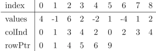
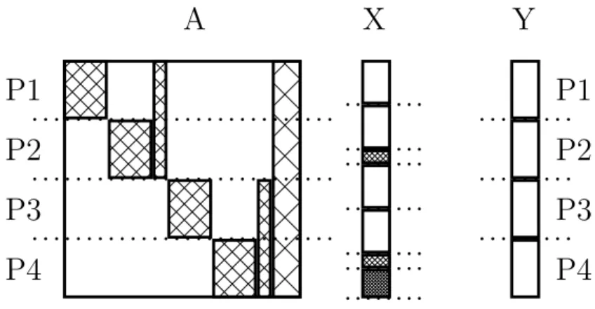
As shown in Figure 2.6, output vector Y is partitioned among 4 PEs which resulted in dividing matrix in row slices and broadcasting input vector X to all processing elements. Rowwise 1-D block partitioning algorithm incurs shared reads on X vector on shared memory architectures.

A

X

Y

P2

P3

P4

P1

P2

P3

P4

P1

Figure 2.6: Rowwise 1-D Block Partitioning algorithm for 4 PEs.

2.2.3.2 Columnwise 1-D Block Partitioning

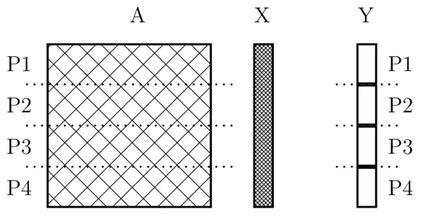
Parallel algorithm for columnwise 1-D block partitioning is similar to rowwise, except this time input vector X is partitioned among PEs which resulted in par-titioning matrix in column slices and collective usage of output vector Y. Paral-lel SpMxV using this type of decomposition incurs conflicting writes and must provide a synchronization infrastructure to guarantee the correctness of results. Columnwise 1-D partitioning algorithm is depicted in Figure 2.7.

(30)

A

X

Y

P1 P2 P3 P4

P1

P2

P3

P4

Figure 2.7: Columnwise 1-D Block Partitioning algorithm for 4 PEs.

2.2.3.3 2-D Block Partitioning

Also known as checkerboard, 2-D block partitioning algorithm directly divides given matrix into blocks in way that both input vector X and output vector Y can be partitioned among all PEs. Both shared reads and conflict writes incurred in this decomposition type. Figure 2.8 shows this scheme in action for 16 PEs.

A

X

Y

P1 P2 P3 P4

P5 P6 P7 P8

P9

P10 P11 P12

P13 P14 P15 P16

Figure 2.8: 2-D Block Partitioning algorithm for 16 PEs.

It is stated in [1] that DMxV multiplication is more scalable with 2-D parti-tioning algorithm. In addition, for SpMxV multiplication, cache blocking tech-niques can be used with checkerboard partitioning.

(31)

This work uses only rowwise 1-D decomposition algorithm.

2.3 Partitioning & Hypergraph model explored

In this study, hypergraph partitioning model [11] serves is used to sort matrix rows and columns so that case misses induced by X vector entries are reduced.

In a single iteration of SpMxV multiplication, SpM entries are used only once. On the other hand, dense vector entries are used multiple times. When combined SpM, Y, and X size is bigger than targeted cache size, vector entries can be evicted from and transferred back to cache due to its limited capacity. Hypergraph partitioning model is utilized to order SpM rows and columns such that vector entries are used multiple times before they are finally evicted from cache.

Secondly, in parallel systems where performance can be hindered by commu-nication and uneven work distribution between PEs (processing elements), with the help of hypergraph partitioning model;

• elegant task decomposition which reduces inter-process comminication, • locality aware scheduling and load balancing algorithms,

can be implemented. PATOH (Partitioning Tool for Hypergraphs) [11] is used throughout this work. Two of PATOH’s partitioning models are explained below.

2.3.1 Column-Net Model & Interpretation

In the column-net model [11], matrix columns are represented as nets (hypern-odes) and rows as vertices. Ordering & Partitioning decisions are made using cut nets which represent columns that cannot be fully assigned to single PE, therefore has to be shared.

(32)

In this work, column-net model is used with rowwise 1-D partitioning algo-rithm which is previously explained in this chapter. SpM entries on borders incur collective reads on shared memory architectures.

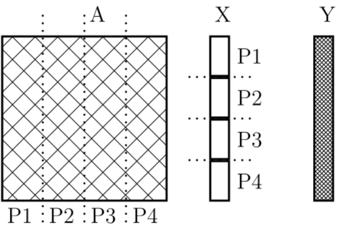
When using column-net interpretation, partitioning a matrix into 2 sub-matrices incurs one column border. In Figure 2.9, sample structure of a sparse matrix partitioned using column-net model is depicted. A1 and A2 are dense blocks (which will be distributed among PEs). B is border which has all the cut nets (columns that cannot be fully assinged to single PE).

Figure 2.9: Column-net interpretation incurs vertical border.

2.3.2 Row-Net Model & Interpretation

In the row-net model [11], matrix rows are used as nets (hypernodes) and columns as vertices. Ordering & Partitioning decisions are made using cut nets which represent rows that cannot be fully assigned to single PE, therefore has to be shared.

When using row-net interpretation, partitioning a matrix into 2 sub-matrices incurs one row border. In Figure 2.10, sample structure of a sparse matrix par-titioned using row-net model is depicted.

(33)

Figure 2.10: Row-net interpretation incurs horizontal border.

Row-net model is not used throughout this work.

2.3.3 Recursive Bipartitioning

PATOH recursively divides a matrix into two sub-matrices until the total size of data structures (required to multiply sub-matrix in question) falls below targeted size (determined by user input). Generally, targeted size is either below or equal to the local cache size of a processor core. This way, number of cache capacity misses are reduced.

Total size of the sub-matrix data structure denpends on the underlying storage format and explained in section 2.2.2

• Rowwise 1-D partitioning algorithm when used with column-net partition-ing model & interpretation,

• Columnwise 1-D partitioning algorithm when used with row-net partition-ing model & interpretation (not used in this work),

produces better load balance and parallel scalability.

In Figures 2.11 and 2.12, both algorithms are depicted in action accordingly. Matrices are partitioned using bipartitioning scheme explained earlier in this chapter.

(34)

A

X

Y

P2

P3

P4

P1

P2

P3

P4

P1

Figure 2.11: A SpM is recursively reordered and divided into four parts using

column-net recursive bipartitioning scheme. And sub-matrix to PE assignment is done using rowwise 1-D partitioning algorithm.

As can be seen from Figure 2.11, using ordering, number of shared reads are reduced compared to Figure 2.6 (Shared portion of X vector are weaved denser).

A

X

Y

P1 P2 P3 P4

P1

P2

P3

P4

Figure 2.12: An SpM is recursively reordered and divided into 4 parts using

row-net recursive bipartitioning scheme. Sub-matrix to processor assignment is done by using columnwise 1-D partitioning algorithm.

Column parallel SpMxV using row net partitioning scheme, as shown in Figure 2.12, reduces the number of conflicting writes (weaved denser), thus the synchro-nization overhead, compared to SpMxV in Figure 2.7 is minimized.

(35)

2.4 A high level overview of Intel’s Xeon Phi

High Performance Computing Platform

Covering the whole architecture of Xeon Phi cards is out of the scope of this document. Therefore, hardware is briefly inspected and only the parts that are crucial for this study are explained in detail.

Xeon Phi co-processor card [13, 14] is an external and independent hardware that works in conjunction with Xeon processor [25]. It’s very similar to GPU in that sense.

Unlike a graphics card, Xeon Phi card has very similar structure to that of a traditional processor, making it easy to program and port existing code written for a conventional processors [3]. Porting is done by Intel’s compiler [3, 23] (thus it is required to program the coprocessor). As a result, using the implementations of algorithms which are designed for traditional processors, speed-up can be attained on Xeon Phi card.

Xeon Phi coprocessor is intended for applications where runtime is dominated by parallel code segments. Because Xeon Phi cores have much lower frequency compared to Xeon cores, tasks whose runtime is dominated by serial execution segments can perform better on general purpose Xeon processors [3]. Specifica-tions of these two products used throughout this work are given in are given in chapter 5.

In addition to 60+ cores, Xeon Phi coprocessor cards;

• use directory based cache coherency protocol compared to Xeon’s bus based cache coherency protocol.

• has 512bit SIMD vector unit in each core, compared to Xeon’s SSE / MMX instructions.

(36)

2.4.1 5 key features of Xeon Phi Coprocessors

Covering features of Xeon Phi Coprocessors is out of the scope of this document. Here are the 5 aspects of this hardware which carries upmost importance for this work.

2.4.1.1 Number of threads per core

Each core has an inorder dual-issue pipeline with 4-way simultaneous multi-threading (SMT). For applications (except the ones that are heavily memory intensive), each core must have at least two threads to attain all the possible per-formance from coprocessor. This is the result of coprocessor cores having 2-stage pipeline and described in [3].

2.4.1.2 On die interconnect

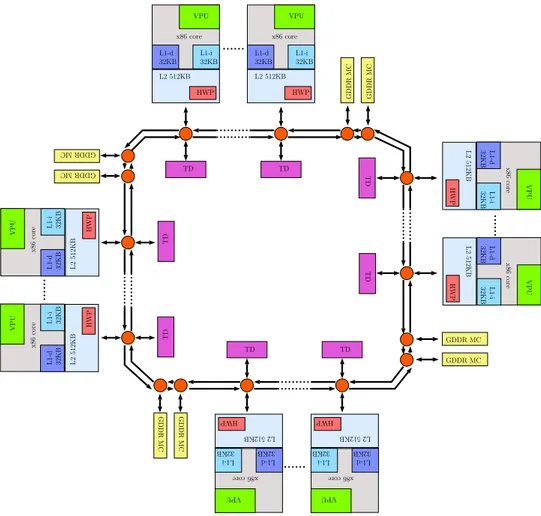
All the processing elements on die are connected to each other with a bidirectional ring which uses store and forward communication scheme (making it possible that one or more messages can be on the ring at the same time). It is mentioned in [3] that, because of high quality design of interconnect, data locality beyond a single core (4 threads running on same core) usually doesn’t make any diﬀer-ence. Meaning the physical distance between two communicating cores doesn’t significantly aﬀect overall performance. See Figure 2.13 for a high level hardware view.

(37)

x86 core VPU L1-i 32KB L1-d 32KB L2 512KB HWP x86 core VPU L1-i 32KB L1-d 32KB L2 512KB HWP GDDR MC GDDR MC x86 core VPU L1-i 32KB L1-d 32KB L2 512KB HWP x86 core VPU L1-i 32KB L1-d 32KB L2 512KB HWP GDDR MC GDDR MC x86 core VPU L1-i 32KB L1-d 32KB L2 512KB HWP x86 core VPU L1-i 32KB L1-d 32KB L2 512KB HWP GDDRMC GDDRMC x86core VPU L1-i 32KB L1-d 32KB L2512KB HWP x86core VPU L1-i 32KB L1-d 32KB L2512KB HWP GDDR MC GDDR MC TD TD TD TD TD TD TD TD

Figure 2.13: High level view of on-die interconnect on Xeon Phi Coprocessor

cards. TD (tag directory), MC (Memory Channel), L2 (Level 2 Cache), L1-d (Level 1 Data Cache), L1-i (Level 1 Instruction Cache), HWP (harL1-dware prefetcher).

There are 3 type of bidirectional rings, each of which is used for diﬀerent purposes and operate independently from one another [27].

• Data block ring: Sharing data among cores.

• Address ring: Send/Write commands and memory addresses. • Acknowledgement ring: Flow control and coherency messages.

(38)

2.4.1.3 Vector Unit

Each core has 512bit wide SIMD instruction unit. Which means 8 double or 16 single precision floating point operations may be carried out at the same time. It can be used in loop vectorization, however as explained in [4] loops must meet the following criterias in order to be vectorized.

1. Countable: Loop trip count must be known at entry of a loop at runtime and remain constant for the duration of the loop.

2. Single entry and single exit: There should be only one way to exit a loop once entered (Use of breaks and data-dependent exit should be avoided). 3. Straight-line code: It is not possible for diﬀerent iterations to have

dif-ferent control flow, in other words use of branching statements should be avoided (However, there is an exception to this rule if branching can be implemented as masked assignments).

4. The innermost loop of a nest: Only the innermost loop will be vec-torized (exception being outer loops transforming into an inner loop from through prior optimization phases).

5. No function calls: There shouldn’t be any procedure call withing a loop (major exceptions being intrinsic math functions and functions that can be inlined).

2.4.1.3.1 Obstacles to vectorization There are certain elements that not

necessarily prevent vectorization, but decrease their eﬀectiveness to a point in which whether to vectorize is questioned. Some of these elements (illustrated detailly in [4]) are described below;

1. Data alignment: To increase the eﬃciency of vectorization loop data should be aligned by the size of architecture’s cache line. This way, it can be brought into cache using minimum amount of memory accesses.

(39)

2. Non-contiguous memory access: Data access pattern of an application is crucial for eﬃcient vectorization. Consecutive loads and stores can be accomplished using single high performance load instruction incorporated in Xeon Phi (or SSE instructions in other architectures). If data is not layed out continuously in memory, Xeon Phi architecture supports scatter and gather instructions which allow manipulation of irregular data patterns of memory (by fetching sparse locations of memory into a dense vector or vice-versa), thus enabling vectorization of algorithms with complex data structures [26]. However, as shown in Section 4.3.2, it is still not as eﬃcient. 3. Data Dependencies: There are 5 cases of data dependency overall in

vectorization.

(a) No-dependency: Data elements that are written do not appear in other iterations of the loop.

(b) Read-after-write: A variable is written in one iteration and read in a subsequent iteration. This is also known as ’flow dependency’ and vectorization can lead to incorrect results.

(c) Write-after-read: A variable is read in one iteration and written in a subsequent iteration. This is also known as ’anti-dependency’ and it is not safe for general parallel execution. However, it is vectorizable. (d) Read-after-read: These type of situations are not really

dependen-cies and prevent neither vectorization nor parallel execution.

(e) Write-after-write: Same variable is written to in more than one iteration. Also refered to as ’output dependency’ and its unsafe for vectorization and general parallel execution.

(f) Loop-carried dependency: Idioms such as reduction are referred to as loop-carried dependencies. Compiler is able to recognize such loops and vectorize them.

As much as advatageous it may seem, significant amount of code is not data parallel, as a result it is quite rare to fill all of the SIMD slots. Considering SIMD instructions are slower than their regular counterparts, vectorization may deteriorate performance when heavily under-utilized.

(40)

2.4.1.4 Execution Models

There are 2 execution models for Xeon Phi co-processors.

1. Native Execution Model: In this model, execution starts and ends on co-processor card. This is usually better choice for applications that doesn’t have long serial segments and IO operations.

2. Oﬄoad Execution Model: This is designed for applications with incon-sistent behaviors throughout their execution. Application starts and ends on processor, but it can migrate to co-processor in between. Intends to execute only the highly parallel segments on co-processor. Using processor simultaneously along with co-processor is also possible in this model.

2.4.2 Thread Aﬃnity Control

In this work, precise thread to core assignment is crucial for better spatial locality and architecture awareness. As mentioned in [9], there are 3 basic aﬃnity types depicted in Figures 2.14, 2.15, and 2.16. Examples have 3 cores with each core having 4 hardware threads, and 6 software threads in total.

(41)

Figure 2.15: Scatter thread aﬃnity control.

(42)

Chapter 3 Partitioning, Scheduling, and

Load Balancing Algorithms

In this chapter,

• developed SpMxV routines,

• utilized task decomposition strategies, and

• implemented scheduling and load balancing algorithms are all explained in detail.

(43)

All of the SpMxV routines developed for this study uses rowwise 1-D parti-tioning algorithm and utilizes PATOH’s column net model to regulate memory access patterns of SpMs. They are listed below.

• Ordering only routines 1. Sequential routine

2. Dynamic OMP Loop routine • Ordering & Blocking routines

1. Static routine

(a) Chunk distribution (b) Scatter distribution 2. OpenMP task routine

(a) Chunk distribution (b) Scatter distribution

3. Global work stealing routine (GWS) 4. Distributed work stealing routine (DWS)

(a) Ring work stealing mode i. Chunk distribution ii. Scatter distribution

iii. Shared queue implementation (b) Tree work stealing mode

i. Chunk distribution ii. Scatter distribution

iii. Shared queue implementation

In the following sections, clarifications about those routines on the way they work and the problems they aim to solve are made.

(44)

3.1 Ordering Only Routines

Routines presented in this category utilize only the ordering information passed on by hypergraph model.

3.1.1 Sequential Routine

Uses traditional sequential SpMxV algorithm on single Xeon Phi core using only one thread. This algorithm is used as a baseline to calculate speed up of other algorithms and forms application kernel for other routines. C style pseudo code of this routine is provided in Algorithm 4.2 and Algorithm 4.3 for both CSR and JDS formats in order.

3.1.2 Dynamic OMP Loop Routine

This is the parallelized version of sequential routine using OpenMP parallel for pragma. Routine distributes sparse-matrix rows by using OpenMP runtime load balancing algorithms (Dynamic scheduling type is chosen using 32, 64, 128 long trip counts). Schedule types are described in [12].

Problem with using OpenMP runtime load balancing algorithms is that

• they don’t use the benefits of cache blocking done by partitioning algo-rithms. Thus may occasionally disturb data locality.

• they can fail to balance workload in cases where a matrix has dense rows & small row count (latter needs a change in scheduling trip count to get fixed).

• they allow limited control over the order in which SpM entries are traversed. Certain storage schemes cannot be implemented inside OpenMP’s parallel for pragma.

(45)

However, unlike routines that use blocking, dynamic implementation doesn’t have the extra for loop (which is used for traversing SpM row slices - also ad-dressed as sub-matrices) overhead.

(46)

3.2 Ordering & blocking routines

In hypergraph partitioning powered use, routines in this category utilize cache blocking techniques along with ordering. Blocking information is either passed on by hypergraph model or created manually in spontaneous mode. Also, the load balancing decisions and initial partitioning in these routines are locality and architecture aware when using hypergraph model. In spontaneous mode, they only consider underlying architecture (physical placement of EXs) before making any scheduling decisions.

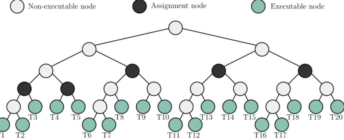
An SpM is partitioned using recursive bipartitioning algorithm explained in chapter 2. Then load balancing decisions are extracted from resulting bipartition-ing tree. Sample bipartitionbipartition-ing tree and its correspondbipartition-ing matrix view (ordered using hypergraph model), shown in Figures 3.1 and 3.2, are used throughout this chapter for more clear explanation of partitioning and scheduling algorithms.

Non-executable node Assignment node Executable node

T1 T2 T3 T4 T5 T6 T7 T8 T9 T10 T11 T12 T13 T14 T15 T16 T17 T18 T19 T20

Figure 3.1: Sample bipartitioning tree for column-net interpretation using

(47)

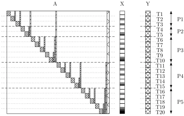
A X Y T2 T3 T4 T1 T6 T7 T8 T5 T10 T9 T11 T12 T13 T14 T15 T16 T17 T18 T19 T20 P1 P2 P3 P4 P5

Figure 3.2: Sample matrix ordered by column-net model using rowwise

1-D partitioning algorithm for task to PE assignment. There are 5 EXs and collective reads on X vector by tasks are pointed out by density of portions’ color.

As mentioned in chapter 2, column-net interpretation is used with rowwise 1-D partitioning. Roles played by each tree node depends on underlying storage scheme, patitioning algorithm, and execution context count as explained below.

• Assignment Node is attached to a PE. All child nodes, connected to this node, are assigned to that PE.

• Non-Executable Node contains a sub-matrix whose total space is bigger than targetted size. So, it is continued to be divided and ignored by PEs. • Executable Node , in rowwise 1-D partitioning, contains a sub-matrix

whose total space is smaller than targetted size. Therefore, it isn’t divided anymore and ready for execution. Additionally, in implementations that have conflicting writes, inner nodes of the bipartitioning tree are also exe-cutable and require synchronization framework. In this study, matrices are

(48)

distributed by rowwise 1-D partitioning algorithm and underlying storage schemes are CSR and JDS, as a result, only the leafs in Figure 3.1 are executable.

Depicted in Figure 3.1 and 3.2, when using hypergraph model, nodes that have more common parents, share more input dense vector entries (borders). Thus, for each EX, executing groups of nodes that share this trait, will result in better performance and such approach is said to be locality aware.

3.2.1 Chunk & Scatter Distribution Methods

Before describing distribution methods, it is mandatory to define a block. In this study, Block is a group of EXs. It can have multiple EXs or single one.

3.2.1.1 Chunk Distribution

In chunk distribution, a block consists of single EX. Assignments to blocks occur as chunks of continuous sub-matrices. For 5 EXs, assignment is the same as the on depicted in Figures 3.1 and 3.2.

3.2.1.2 Scatter Distribution

In scatter distribution, a block can have multiple EXs. It is assumed that EXs on the same block is physically closer to each other than other EXs. Therefore, continuous sub-matrices are scattered among multiple EXs in a block. When execution starts, each EX executes the sub-matrices that share the most X vector entries, at the same time in an eﬀort to improve temporal locality. In Figures 3.3 and 3.4 this distribution method is shown in action for 2 blocks, first containing 3 EXs, while the latter having only 2.

(49)

Non-executable node Assignment node Executable node T1 T2 T3 T4 T5 T6 T7 T8 T9 T10 T11 T12 T13 T14 T15 T16 T17 T18 T19 T20

Figure 3.3: Bipartitioning tree for 2 blocks.

A X Y T2 T3 T4 T1 T6 T7 T8 T5 T10 T9 T11 T12 T13 T14 T15 T16 T17 T18 T19 T20 P1 P2 P3 P4 P5

Figure 3.4: Sample matrix ordered by column-net model using rowwise 1-D

partitioning using scatter distribution method. Collective reads by task on X vector are shown by the density of potions’ color.

(50)

3.2.2 Static Routine

This routine makes use of cache blocking techniques to adjust size of sub-matrices which reduces the number of cache capacity misses. Figure 3.5 shows how initial work distribution is done in block parallel algorithm.

Non-executable node Assignment node

Job batch Job queue

Figure 3.5: Static routine sub-matrix distribution among 5 execution

con-texts.

When used with hypergraph partitioning, tasks who share more borders (X vector entries) are assigned to a single PE as shown in Figures 3.2 and 3.5.

The downside of static routine is that it only uses initial work distribution to balance load. Throughout execution no scheduling decisions are made which causes load imbalance as shown in Figure 3.5.

(51)

3.2.3 OpenMP Task Routine

Tries to improve static routine by adding a dynamic load balancing component. After an EX finishes its share of load, it looks to steal from other EXs and choses the victim randomly. Since this routine is implemented using omp task pragma, control of the order in which sub-matrices are executed and the victim choice is left to OpenMP runtime.

Aside from locking schemes used by OpenMP runtime, this routine tries to improve load balance without destroying cache blocks. In this work, victim choice can improve performace (in both hypergraph partitioning and sponta-neous modes). However, lacking a way to control execution order, steal count (how many matrices to steal at once), and choosing the victim randomly this methods doesn’t allow further tuning.

(52)

3.2.4 Global Work Stealing Routine (GWS)

GWS uses a single FIFO job queue, accessed multiple times by and EX, as a means of dynamic load balancing structure. In GWS, all the sub-matrices are stored in a global queue, and each EX takes the first sub-matrix from queue as they finish the sub-matrix they are currently working on. Queue is protected by a single spin lock which has to be obtained in order to make a change in its state. In Figure 3.6 the way sub-matrices line up in global queue is depicted.

Non-executable node Assignment node Job batch Job queue Global Job Queue

Figure 3.6: Global queue and the order in which sub-matrices line up.

Although using a global job queue provides perfect load balance, it also limits scalability since all EXs are racing to obtain the same lock. It can also be argued that it destroys data locality of initial work distribution.

(53)

3.2.5 Distributed Work Stealing Routine (DWS)

Instead of a single FIFO queue, this algorithm keeps multiple FIFO queues, 1 per EX, each protected by its own lock. A block can have either 1 or more EXs depending on diﬀerent DWS implementations (See Chapter 4). Initial state of the queues before execution are same as Figure 3.5. To preserve data-locality in victim queues, successful steal attempts to a queue always removes tasks from the back. Not front, where owner of the queue detaches tasks for itself.

Stealing in this routine happens in 2 ways.

3.2.5.1 Ring Work Stealing Scheme

This scheme is designed to make better use of ring based communication inter-connect and it is locality aware in a sense that it checks for nearby cores first. In Figure 3.7, it is shown in action.

n.th victim Finished PE 1 2 3 5 7 4 6 8 58 59 57 55 53 56 54 52 n

Figure 3.7: Ring work stealing scheme making eﬃcient use of bidirectional

communication ring for 60 PEs.

True data-locality awareness in ring stealing scheme comes from the hyper-graph partitioning phase. Because of the way sub-matrices are distributed, there

(54)

is a strong chance that nearby EX carry sub-matrices using more common input dense vector entrice compared to a distant EX.

This algoirthm is also architecture aware since each EX prefers steal attempts on nearby EXs (in terms of physical placement) over distant ones in an eﬀort to relax communication volume.

3.2.5.2 Tree Work Stealing Scheme

This scheme is more aggressive in a sense that it tries harder to steal the sub-matrices with more common input dense vector entries. It uses bi-partitioning tree to look for victims without any concerns for on-die interconnect. Figure 18 shows this scheme in action.

Non-executable node Assignment node P1 P2 P3 P4 P5 Victim Orders P1: 2 3 5 4 P2: 1 3 5 4 P3: 2 1 5 4 P4: 5 3 2 1 P5: 4 3 2 1

Figure 3.8: Tree work stealing scheme in action.

This algorithm too is locality aware since it prefers stealing sub-matrices with more common borders first.

Compared to GWS, DWS algorithm is more scalable because, contention for each EXs’ lock is much less compared to global lock contention of GWS. On the

(55)

downside, EXs still have to go through a lock for accessing their local queues which limits application scalability.

In distributed schemes, after a victim is chosen, last half of the tasks in its local queue are stolen. However, execution contexts don’t perform steals on queues which has less than certain number of entries. This is called steal treshold and is an adjustable parameter.

3.2.5.3 Shared Queue Implementation

Everything is same with chunk distribution except in shared queue implemen-tation blocks have more than one EX sharing the same job queue and stealing occurs between blocks. The first EX that spots the job queue is empty, will look to steal from other blocks while other EXs in the same block stalls. After a suc-cessful steal attempt, EX that stole sub-matrices will get itself a single sub-matrix and free synchronization units for others to continue execution.

Much like scatter distribution, EXs on the same block are assumed be closer in terms of physical placement and temporal data locality is tried to be exploited. This implementation, however, is more strict from scatter distribution in that data-locality is restricted to single block until that blocks sub-matrices are all executed. After that, stealing can be accomplished according to both ring and tree work stealing designs.

This implementation of DWS is designed to be used with hypergraph parti-tioning which is employed to regulate memory access pattern of SpMs.

(56)

Chapter 4 Implementation deltails, Porting,

and Fine tuning

In this chapter;

• high level execution course of application, • detailed analysis of application kernels, • optimization techniques used,

• new hybrid storage scheme for sub-matrices and an algorithm to extract it are presented.

(57)

4.1 Test sub-set

Peak GFlops achieved for each proposed routine on test SpM set of this work are given in chapter 5. Because there are more than 200 test results, to demonstrate the eﬀects of optimizations documented in this chapter, small but diverse sub-set of 15 matrices are chosen. Below in Table 4.1, stats of these matrices are presented.

Table 4.1: Stats of choosen data sub-set. Row & column count, NNZ, and

max-avg-min NNZ per row/column are given.

row column

Matrix rows columns nnz min avg max min avg max

3D 51448 3D 51448 51448 1056610 12 20.5 5671 13 20.5 946 3dtube 45330 45330 3213618 10 70.9 2364 10 70.9 2364 adaptive 6815744 6815744 20432896 1 3 4 0 3 4 atmosmodd 1270432 1270432 8814880 4 6.9 7 4 6.9 7 av41092 41092 41092 1683902 2 41 2135 2 41 664 cage14 1505785 1505785 27130349 5 18 41 5 18 41 cnr-2000 325557 325557 3216152 0 9.9 2716 1 9.9 18235 F1 343791 343791 26837113 24 78.1 435 24 78.1 435 Freescale1 3428755 3428755 18920347 1 5.5 27 1 5.5 25 in-2004 1382908 1382908 16917053 0 12.2 7753 0 12.2 21866 memchip 2707524 2707524 14810202 2 5.5 27 1 5.5 27 road central 14081816 14081816 19785010 0 1.4 8 0 1.4 8 torso1 116158 116158 8516500 9 73.3 3263 8 73.3 1224 webbase-1M 1000005 1000005 3105536 1 3.1 4700 1 3.1 28685 wheel 601 902103 723605 2170814 1 2.4 602 2 3 3

Optimizations in this chapter doesn’t alter matrix structures in any way. They are, in general, related to (parallel) programming and geared towards eﬀective usage of host hardware resources. To demonstrate their impact more clearly, results are presented in between.

(58)

4.2 General template of application behaviour

Explanations of sub-routines ,shown in Algorithm 4.1, are listed below;

1. CREATE SUB MATRICES procedure divides SpM into smaller parts and its implemention changes with underlying storage scheme.

2. ASSIGN TO EXs procedure performs the initial assignment has diﬀerent implementation for each routine explained in chapter 3

3. ADAPTIVE WARM UP procedure adaptively balances workload be-tween multiple execution contexts and is also diﬀers for routines mentioned in chapter 3.

4. EXECUTE KERNEL procedure performs SpMxV and varies depend-ing on underlydepend-ing storage scheme and task decompoisition as explained in section 4.3.

Algorithm 4.1 General template of application behaviour.

1: A← sparse matrix

2: ▷ Cache size for sub-matrices are calculated using total size of the partial spm strucutre and size of corresponding output vector entries

3: cacheSize← targettedsize

4: ex count← total number of execution contexts

5: sub mtx list← ROW W ISE 1D P ART IT ION(A, cacheSize)

6: initial assignments← ASSIGN T O EXs(sub mtx list, ex count)

7: assignments← ADAP T IV E W ARM UP (initial assignments, ex count)

8:

9: P arallelSection

10: ex id← ID of current execution context

11: ex subM atrices← assignments(ex id)

12: while ex-subMatrices is not empty do

13: subM atrix← ex subMatrices.remove()

14: EXECUTE KERNEL(subMatrix, x, y)

(59)

4.3 Application Kernels

Impelementation details and aplication kernels for CSR and JDS formats are given in next two sections.

4.3.1 CSR format

In CSR implementation, sub-matrix structure composed only of a descriptor which includes, starting row index, row count, starting column index, and column count of sub-matrix itself.

Task decomposition depicted in Figure 4.1 occurs in row slices and during multiplication process global SpM structure is used with sub-matrix descriptors.

Column count

Row count Starting Row Index

Starting Column Index

Figure 4.1: Task decomposition for CSR format.

Kernel function for CSR format is given in Algorithm 4.2. For SpMs having only a few average non-zero elements per row (smaller than SIMD length), CSR scheme suﬀers from vectorization since most of SIMD slots will be left unutilized. However, this scheme will benefit from vector component considering SpM rows are dense enough to eﬀectively fill SIMD slots.

(60)

Algorithm 4.2 Kernel function for CSR format.

1: _{function CSR KERNEL(csr, x, y)}

2: for i = 0; i≤ csr.rowCount; + + i do

3: sum← 0

4: for j = csr.rowP tr[i]; j ≤ csr.rowP tr[i + 1]; + + i do

5: sub← sum + csr.values[j] ∗ x[csr.colInd[j]];

6: end for

7: y[i]← sum;

8: end for

9: end function

4.3.2 JDS format

As depicted in Figure 4.2 task decomposition is implemented as row slices. How-ever, in addition to a descriptor, sub-matrix strucutres also has a part of SpM stored in JDS format (partial JDS). And during multiplication, this structure is used instead of global SpM.

Column count

Row count Starting Row Index

Starting Column Index

Partial JDS idiag [ ] jdiag [ ] values [ ]

(61)

Kernel function for JDS format is given in Algorithm 4.3. As mentioned in section 2.2.1, for well behaved matrices, JDS format can be vectorized eﬃciently. On the other hand, for SpMs that have occasional dense rows and significantly low average non-zero count per row, vectorization becomes ineﬃcient. Because vectorization is carried out by unrolling the innermost loop of JDS kernel, loop will most likely have very few iterations when traversing dense rows. Therefore, the mojority of SIMD slots will be left empty.

Algorithm 4.3 Kernel function for JDS format.

1: _{function JDS KERNEL(jds, x, y)}

2: for i = 0; i≤ jds.idiagLength; + + i do

3: for j = jds.idiag[i]; j ≤ jds.idiag[i + 1]; + + j do

4: rowIndex← j − jds.idiag[i];

5: y[jds.perm[rowIndex]+ = jds.dj[j]∗ x[jds.jdiag[j]];

6: end for

7: end for

8: end function

Application kernel for JDS can be further optimized by making memory ac-cesses to y vector sequential. In optimized implementation permuataion array in JDS structure is eliminated by one time sort on y vector at the end of multipli-cation phases. Performance diﬀerences regarding the update are given in Table 4.2.

(62)

Table 4.2: Eﬀect of discarding permutation array from JDS format. Results

are measured in GFlops and belong to single precision spontaneous static rou-tine with 32KB sub-matrix sizes. Gains are substantial for matrices that are eﬃciently vectorizable.

jds perm jds sort

Matrix (GFlops) (GFlops)

3D 51448 3D 0.30 0.33 3dtube 1.64 1.97 adaptive 3.63 4.20 atmosmodd 13.89 16.48 av41092 0.67 0.34 cage14 5.47 6.33 cnr-2000 3.79 4.65 F1 2.58 2.90 Freescale1 3.00 3.23 in-2004 1.71 1.87 memchip 7.09 3.54 road central 0.65 0.67 torso1 0.31 0.32 webbase-1M 0.26 0.28 wheel 601 1.46 0.65

(63)

4.4 Runtime Scheduling and Load Balance

4.4.1 Generic Warm-up Phase

Each routine, whether it is ordering only or uses both ordering and blocking, is run 10 times to warm up CPU caches. In this work, SpMxV operation usually takes up much more space than the space provided by CPU caches as a direct result of huge SpM size. Therefore, SpM, X, and Y vector entries cannot reside in cache between runs. However, generally, warm-up operation is not designed for data-sets, but for frequently used data-structures that are small enough to fit into cache, such as job queues. After warm-up stage, application simply settles down on hardware.

4.4.2 Improving Application Scalability

Routines implemented using ’OpenMP for loop’ limits programmers’ control in many ways as described in Chapter 3. Therefore, they do not allow any more tuning in warm-up phase.

However, routines with hand coded scheduling algorithms can be optimized during warm-up phase. When each routine is executed multiple times, frequently used job-queue data structures, thread descriptors, and other low level primitives such as scheduling data structures are brought into cache so that each routine can settle down.

Routines with dynamic scheduling rely on lock and other synchronization primitives defined by OpenMP library to ensrure correctness of results. Although it depends on routines itself, synchronization overhead introduced by locks is visible in every routine and significantly limits scalability of an application. Locks aﬀect GWS the most because of contenttion caused by all EXs racing to obtain a single lock. As a result, it cannot scale up to 240 threads which is the most number of threads, Xeon Phi model used in this work can simultaneously run.

(64)

As for distributed routines, although contention per lock is greatly reduced, PEs still have to go through their own lock to access local queue which significantly hinders performance. There is litte improvement between 180 threads (3 per core) and 240 (4 per core). By discarding these locks and critical sections, hardware threads will not be stalled due to yields caused by them.

Also, locks and other sychronization primitives used by handcoded schedulers are defined at a relatively high level (also called as application-level), which incurs more overhead than sometimes needed (as they are designed for general use) [28]. For SpMxV, all this can be discarded through warm-up phase. Execution starts with initial task decompositions which are defined in Chapter 3. After a run, stolen tasks for each queue are recorded and job queues are reformed using that info. And for the next run, same thing happens on reformed job queues. This phase is repeated for 10 times, where each run building on the one before it. It has been observed that after 6 - 7 runs, job queues reach to an almost stable state, where task groups assigned to PEs, do not change despite actively working scheduler. Consequently, number of times software threads yield due to I/O are reduced and scalability is further enhanced. This is called adaptive warm-up phase, since it displays a form of learning.

4.4.3 Adaptiveness: Reasoning

Previously, when performance was limited by the transistor count (calculation power) of processor, load balance could be defined as “equally distributing

computations to each processing element”. However, today, where

major-ity of applications’ performance is determined by their memory access pattern, it is almost mandatory to alter the definition by adding “and minimizing

pro-cessing element idle time”. To further illustrate the point, below in Table

(65)

Table 4.3: Row & Column count, NNZ, and max, avg, min NNZ per row/column are given for as-Skitter and packing-500x100x100-b050.

Matrix rows columns nnz row column

min avg max min avg max

as-Skitter 1696415 1696415 20494181 0 12.1 35455 0 12.1 35455

packing-500x

2145852 2145852 32830634 0 15.3 18 0 15.3 18

100x100-b050

From Table 4.3, it can be seen that as-Skitter has lesser NNZ. It also has smaller row & column count which translates into Y & X vector sizes respec-tively. Bigger Y vector also means number of writes are higher. However, packing-500x100x100-b050 is more structured since there isn’t big diﬀerence be-tween max/avg/min NNZ per row & column. Below in Table 4.4 results of 100 SpMxV operations for these matrices are presented for both spontaneous & hy-pergraph powered uses for Static and DWS routines.

Table 4.4: Time measured (in seconds) for 100 SpMxV operations performed

using as-Skitter and packing-500x100x100-b050 with Static and DWS routines both ’sp’ (spontaneous) and ’hp’ (hypergraph) modes. ’spc’ stands for spon-taneous mode partition count while ’hpc’ for hypergraph mode patition count. In third row, how many times faster packing-500x100x100-b050 executes com-pared to as-Skitter is shown. (A hybrid storage format, proposed later in this chapter, is used to take these runs).

Matrix spc hpc static DWS

sp hp sp hp

as-Skitter 3959 2606 1.589 0.577 0.531 0.372

packing-500x100x100-b050 8192 4139 0.378 0.279 0.227 0.255

comparison - speedup 4.20 2.06 2.33 1.45

Compared to packing-500x100x100-b050, as-Skitter also has much less par-tition count. However, because of its complex structure, as-Skitter’s memory

Parallel sparse matrix vector multiplication techniques for shared memory architectures

PARALLEL SPARSE MATRIX VECTOR

MULTIPLICATION TECHNIQUES FOR

SHARED MEMORY ARCHITECTURES

a thesis

submitted to the department of computer engineering

and the graduate school of engineering and science

of bilkent university

in partial fulfillment of the requirements

for the degree of

master of science

By

Mehmet Ba¸saran

September, 2014

ABSTRACT

PARALLEL SPARSE MATRIX VECTOR

MULTIPLICATION TECHNIQUES FOR SHARED

MEMORY ARCHITECTURES

¨

OZET

PAYLAS

¸IMLI HAFIZA S˙ISTEMLER˙I ˙IC

¸ ˙IN PARALEL

SEYREK MATR˙IS - D˙IZ˙I C

¸ ARP˙IM TEKN˙IKLER˙I

Acknowledgement

Contents

List of Figures

List of Tables

List of Algorithms

Chapter 1

Introduction

1.1

Preliminary

1.2

Problem Definition

1.3

Thesis Organization

Chapter 2

Background

2.1

Terms and Abbreviations

2.2

Background Infomation on SpMxV

2.2.1

Sparse-Matrix Storage Schemes

2.2.2

Space Requirements

2.2.3

Task decomposition techniques for SpMxV

A

X

Y

P2

P3

P4

P1

P2

P3

P4

P1

A

X

Y

P1 P2 P3 P4

P1

P2

P3

P4

A

X

Y

P1 P2 P3 P4

P5 P6 P7 P8

P9

P10 P11 P12

P13 P14 P15 P16

2.3

Partitioning & Hypergraph model explored

2.3.1