Başlık: Modified unscented Kalman Filter for nonlinear systems having linear subsystems Yazar(lar):BABACAN KOKSAL, Esin; DOROSLOVACKI, Milos I.; ÖZBEK, LeventCilt: 64 Sayı: 2 Sayfa: 089-098 DOI: 10.1501/Commua1_0000000736 Yayın Tarihi: 2015 PDF

Volume 64, Number 2, Pages 89-98 (2015) DOI: 10.1501/commua1-2_0000000736 ISSN 1303-5991

Received by the Editors: August 28, 2015; Accepted: November 16, 2015.

Key words: Nonlinear Dynamic System, System idendification, Extended Kalman Filter, Unscented Kalman Filter.

© 2015 Ankara University

MODIFIED UNSCENTED KALMAN FILTER FOR NONLINEAR SYSTEMS

HAVING LINEAR SUBSYSTEMS

ESIN KOKSAL BABACAN, MILOS I. DOROSLOVACKI AND LEVENT ÖZBEK

ABSTRACT. The Extended Kalman Filter (EKF) is the often used filtering algorithm for nonlinear systems. But it does not usually produce desirable results. Recently a new nonlinear filtering algorithm named as Unscented Kalman Filter (UKF) is introduced. In this paper, we propose a new modified Unscented Kalman Filter (MUKF) algorithm for nonlinear stochastic systems that are linear in some components. These nonlinear systems can be considered as having linear subsystems with parameters and aim is to estimate the system parameters. In simulation study, performance of the EKF, its known variant Modified Extended Kalman Filter (MEKF), UKF and the proposed MUKF is demonstrated for a nonlinear system that is linear in some components. The results show that MUKF gives the best solution for parameter identification problem.

1.

INTRODUCTION

Discrete-time filtering for nonlinear dynamic system is an important research area and attracted

considerable interest [1]. The most common way of applying the Kalman Filter to a nonlinear system

is in the form of the Extended Kalman Filter (EKF). EKF is based on linearization of the state

equations at each time step and on the use of linear estimation theory [2]. However, it has two known

drawbacks: (1) the first-order linearization can introduce large errors in mean and covairance of the

state vector and (2) the derivation of Jacobian matrices is nontrivial in many applications [2].

Recently, a relatively new nonlinear filtering algorithm named Unscented Kalman Filter (UKF)

is proposed as an improvement to EKF [3]. UKF is based on the unscented transformation, which

uses a set of appropriately chosen weighted sigma points to estimate the means and covariances of

probability distributions. It is not necessary to calculate Jacobians and so the algorithm has superior

implementation properties to the EKF [4].

The UKF is widely used in practice: target tracking [3], position determination [5], multi-sensor

fusion [6] and training of neural networks [7].

ESIN KOKSAL BABACAN, MILOS I. DOROSLOVACKI AND LEVENT ÖZBEK

In [8] it is shown that for a nonlinear system that is linear in some components, a modification

of the EKF

improves the filter performance. This filter has two parallel algorithms and the

modification is achieved by an improved linearization. Algorithm I is a modification of the EKF, in

which the real-time linear Taylor approximation is taken at the optimal state estimate which is given

by the standard KF of the linear subsystem from Algorithm II. The standard KF is obtained by

plugging parameter values estimated by Algorithm I. The MUKF is motivated by the MEKF. In this

paper we want to investigate whether similar modification of the UKF improves the filter

performance or not.

This paper is organized as follows. In Section 2 nonlinear state-space models are described and

brief summary of the UKF algorithm is given. In Section 3 MUKF procedure is introduced. In Section

4 the performance of the EKF, MEKF, UKF and the proposed MUKF is analyzed with a simulation

example. Section 5 is the conclusion.

2.

UNSCENTED KALMAN FILTER

Consider the following nonlinear discrete-time stochastic system

𝑥(𝑘) = 𝑓(𝑥(𝑘 − 1)) + 𝑤(𝑘)

𝑧(𝑘) = ℎ(𝑥(𝑘)) + 𝑣(𝑘)

(1)

where 𝑥(𝑘) (𝑛 − vector) and 𝑧(𝑘) (𝑚 − vector) denote the state and measurement vectors at time

instant 𝑘, 𝑤(𝑘) and 𝑣(𝑘) are uncorrelated zero-mean Gaussian white noise processes with covariance

𝐸(𝑤(𝑘)𝑤

_{(𝑘)) = 𝑄(𝑘), 𝐸(𝑣(𝑘)𝑣}

_{(𝑘)) = 𝑅(𝑘). (2)}

UKF is using a minimal set of determinate sample points (sigma points) to completely

capture the true mean and covariance of the states via Unscented Transformation (UT). UKF

equations are summarized as follows [9]:

A1. Given the state estimate

𝑥̂(𝑘 − 1) and the error covariance matrix 𝑃(𝑘 − 1), the sigma points are

formed by

{

𝜒

(𝑘 − 1) = 𝑥̂(𝑘 − 1) , 𝑖 = 0

𝜒

(𝑘 − 1) = 𝑥̂(𝑘 − 1) + 𝑎 (√𝑛𝑃(𝑘 − 1))

, 𝑖 = 1, … , 𝑛

𝜒

(𝑘 − 1) = 𝑥̂(𝑘 − 1) − 𝑎 (√𝑛𝑃(𝑘 − 1))

, 𝑖 = 𝑛 + 1, … ,2𝑛

(3)

where 𝑎 determines the spread of the sigma points around 𝑥̂(𝑘 − 1) and usually set to a small

positive value. (√𝑛𝑃(𝑘 − 1))

𝑖

is the 𝑖 − th row or column of the matrix square root of 𝑛𝑃(𝑘 − 1).

A2. Prediction: These sigma points are instantiated through the process model to yield a set of

transformed samples

The predicted mean and covariance are computed by

𝑥̂(𝑘|𝑘 − 1) = ∑ 𝑤

𝜒

(𝑘|𝑘 − 1)

(5)

𝑃(𝑘|𝑘 − 1) = ∑ 𝑤

(𝜒

(𝑘|𝑘 − 1) − 𝑥̂(𝑘|𝑘 − 1))

× (𝜒

(𝑘|𝑘 − 1) − 𝑥̂(𝑘|𝑘 − 1))

+ 𝑄(𝑘) (6)

with weights 𝑤

, 𝑤

, … , 𝑤

∈ 𝑅

satisfying ∑

𝑤

= 1 given by

{

𝑤

= 1 −

1

𝑎2

,

𝑖 = 0

𝑤

=

,

𝑖 = 1, … ,2𝑛

. (7)

A3. Update: Given the weighted mean of these transformed sigma points

𝑥̂(𝑘|𝑘 − 1) and the

prediction covariance matrix 𝑃(𝑘|𝑘 − 1), the new sigma points 𝜒

_{(𝑘|𝑘 − 1) are computed as}

{

𝜒

(𝑘|𝑘 − 1) = 𝑥̂(𝑘|𝑘 − 1) , 𝑖 = 0

𝜒

(𝑘|𝑘 − 1) = 𝑥̂(𝑘|𝑘 − 1) + 𝑎 (√𝑛𝑃(𝑘|𝑘 − 1))

, 𝑖 = 1,2, … , 𝑛

𝜒

(𝑘|𝑘 − 1) = 𝑥̂(𝑘|𝑘 − 1) − 𝑎 (√𝑛𝑃(𝑘|𝑘 − 1))

, 𝑖 = 𝑛 + 1, 𝑛 + 2, … ,2𝑛

(8)

The sigma points for the measurements are

𝒵

(𝑘) = ℎ(𝜒

(𝑘|𝑘 − 1)). (9)

The weighted mean and covariance matrix of the predicted observation is given by

𝑧̂(𝑘) = ∑ 𝑤

𝒵

(𝑘)

(10)

𝑃

(𝑘) = ∑ 𝑤

(𝒵

(𝑘) − 𝑧̂(𝑘))(𝒵

(𝑘) − 𝑧̂(𝑘))

+ 𝑅(𝑘)

(11)

and the covariance matrix between the state and the measurement is computed as follows

𝑃

(𝑘) = ∑

𝑤

(𝜒

(𝑘|𝑘 − 1) − 𝑥̂(𝑘|𝑘 − 1)) × (𝒵

(𝑘) − 𝑧̂(𝑘))

𝑇

. (12)

Then the state estimate 𝑥̂(𝑘) and the corresponding covariance matrix 𝑃(𝑘) can be updated by

ESIN KOKSAL BABACAN, MILOS I. DOROSLOVACKI AND LEVENT ÖZBEK

𝑥̂(𝑘) = 𝑥̂(𝑘|𝑘 − 1) + 𝑃

(𝑘)𝑃

(𝑘)(𝑧(𝑘) − 𝑧̂(𝑘)) (13)

𝑃(𝑘) = 𝑃(𝑘|𝑘 − 1) − 𝑃

(𝑘)𝑃

(𝑘)𝑃

(𝑘) . (14)

A4. Repeat steps 1 to 3 for the next sample.

3.

MODIFIED UKF

In this section, with motivation to improve the performance of the UKF for the special form of

nonlinear systems having linear subsystems, we will describe a modification of the UKF similar to

modification of the EKF which was recommended in [8]. It uses two parallel algorithms (Algorithm

I and II). The nonlinear model assumed by MUKF is described as follows. Let 𝑥(𝑘) and 𝑦(𝑘) be 𝑛 −

vector and 𝑚 − vector, and the state vector of the system be the (𝑛 + 𝑚) − vector [𝑥

_{(𝑘) 𝑦}

_(𝑘)]

such that it satisfies

[

𝑥(𝑘 + 1)

𝑦(𝑘 + 1)

] = [

𝐹

(𝑦(𝑘))𝑥(𝑘)

𝐺

(𝑥(𝑘), 𝑦(𝑘))

] + [

𝜉

(𝑘)

𝜉

(𝑘)

]

𝑧(𝑘) = [𝐻

(𝑥(𝑘), 𝑦(𝑘))

0] [

𝑥(𝑘)

_𝑦(𝑘)

] + 𝜂(𝑘).

(15)

[𝜉

_{(𝑘) 𝜉}

2𝑇

(𝑘)]

and 𝜂(𝑘) are uncorrelated zero-mean Gaussian white noise sequences with variance

matrices

𝑄(𝑘) = 𝑉𝑎𝑟 ([

𝜉

(𝑘)

𝜉

(𝑘)

]), 𝑅(𝑘) = 𝑉𝑎𝑟(𝜂(𝑘)) (16)

respectively. 𝐹

, 𝐺

, 𝐻

are nonlinear matrix valued functions.

With motivation to improve the performance, in Algorithm I, the sigma points are evaluated at

the optimal state estimation 𝑥̂(𝑘 − 1) which is determined by the standard KF (Algorithm II) of the

subsystem

𝑥(𝑘 + 1) = 𝐹

(𝑦̃(𝑘))𝑥(𝑘) + 𝜉

(𝑘)

𝑧(𝑘) = 𝐻

(𝑥̃(𝑘), 𝑦̃(𝑘))𝑥(𝑘) + 𝜂(𝑘)

(17)

of (15) evaluated at the estimate

(𝑥̃(𝑘), 𝑦̃(𝑘)) from Algorithm I. Two algorithms are applied in

parallel starting with the same initial estimate. Algorithm I is used yielding the

estimate [𝑥̃

_{(𝑘) 𝑦̃}

_(𝑘)]

_{with the input 𝑥̂(𝑘 − 1) obtained from Algorithm II (Standard KF for the}

linear system) and Algorithm II is used for yielding the estimate 𝑥̂(𝑘) with the inputs ỹ(𝑘 − 1) and

[𝑥̃

_{(𝑘|𝑘 − 1) 𝑦̃}

_{(𝑘|𝑘 − 1)]}

_{obtained from Algorithm I. Algorithm I and Algorithm II are given}

Algorithm I.

[

𝑥̃(0)

𝑦̃(0)

] = [

𝐸(𝑥(0))

𝐸(𝑦(0))

], 𝑃(0) = 𝑉𝑎𝑟 ([

𝑥(0)

𝑦(0)

])

A1.The sigma points are formed by

{

𝜒

(k − 1) = [

x̂(k − 1)

_{ỹ(k − 1)}

] ,

𝑖 = 0

𝜒

(k − 1) = [

x̂(k − 1)

ỹ(k − 1)

] + 𝑎 (√(𝑛 + 𝑚)𝑃(𝑘 − 1))

, 𝑖 = 1,2, … , 𝑛 + 𝑚 (18)

𝜒

(k − 1) = [

x̂(k − 1)

_{ỹ(k − 1)}

] − 𝑎 (√(𝑛 + 𝑚)𝑃(𝑘 − 1))

𝑖 = 𝑛 + 𝑚 + 1, … ,2(𝑛 + 𝑚)

A2.

𝜒

(k|k − 1) = [

F

([𝜒

(k − 1)]

)[𝜒

(k − 1)]

G

(𝜒

(k − 1))

]

[

x̃(k|k − 1)

ỹ(k|k − 1)

] = ∑ W

𝜒

(k|k − 1)

(19)

𝑃(k|k − 1) = ∑ W

[𝜒

(k|k − 1) − [

x̃(k|k − 1)

_{ỹ(k|k − 1)}

]]

× [𝜒

(k|k − 1) − [

x̃(k|k − 1)

ỹ(k|k − 1)

]]

+ 𝑄(𝑘)

where [𝜒

(. )]

is part of the vector related to x̂(. ), and [𝜒

(. )]

is part of the vector related to ỹ(. ).

A3.

{

𝜒

(k|k − 1) = [

x̃(k|k − 1)

ỹ(k|k − 1)

] ,

𝑖 = 0

𝜒

(k|k − 1) = [

x̃(k|k − 1)

ỹ(k|k − 1)

] + 𝑎 (√(𝑛 + 𝑚)𝑃(𝑘|𝑘 − 1))

, 𝑖 = 1,2, … , 𝑛 + 𝑚

𝜒

(k|k − 1) = [

x̃(k|k − 1)

ỹ(k|k − 1)

] − 𝑎 (√(𝑛 + 𝑚)𝑃(𝑘|𝑘 − 1))

, 𝑖 = 𝑛 + 𝑚 + 1, … ,2(𝑛 + 𝑚)

𝒵

(𝑘) = 𝐻

(𝜒

(k|k − 1))

𝑧̂(𝑘) = ∑ W

𝒵

(𝑘)

ESIN KOKSAL BABACAN, MILOS I. DOROSLOVACKI AND LEVENT ÖZBEK

𝑃

(𝑘) = ∑ W

(𝒵

(𝑘) − 𝑧̂(𝑘))(𝒵

(𝑘) − 𝑧̂(𝑘))

+ 𝑅(𝑘)

(20)

𝑃

(𝑘) = ∑ W

(𝜒

(k|k − 1) − [

x̃(k|k − 1)

_{ỹ(k|k − 1)}

])

× (𝑧(𝑘) − 𝑧̂(𝑘))

[

x̃(k)

ỹ(k)

] = [

x̃(k|k − 1)

ỹ(k|k − 1)

] + 𝑃

(𝑘)𝑃

(𝑘)(𝑧(𝑘) − 𝑧̂(𝑘))

𝑃(𝑘) = 𝑃(𝑘|𝑘 − 1) − 𝑃

(𝑘)𝑃

(𝑘)𝑃

(𝑘)

Algorithm II.

𝑥̂(0) = 𝐸(𝑥(0)), 𝑃(0) = 𝑉𝑎𝑟(𝑥(0))

𝑃(k|k − 1) = [𝐹

(ỹ(k − 1))]𝑃(𝑘 − 1) × [𝐹

(ỹ(k − 1))]

+ 𝑄(𝑘 − 1)

x̂(k|k − 1) = 𝐹

(ỹ(k − 1))x̂(k − 1) (21)

𝐾(𝑘) = 𝑃(k|k − 1)[𝐻

(x̃(k|k − 1), ỹ(k|k − 1))]

× {[𝐻

(x̃(k|k − 1), ỹ(k|k − 1))]𝑃(k|k − 1) + 𝑅

}

𝑃(𝑘) = {𝐼 − 𝐾(𝑘)[𝐻

(x̃(k|k − 1), ỹ(k|k − 1))]}

× 𝑃(k|k − 1)

x̂(k) = x̂(k|k − 1) + 𝐾(𝑘) ×

{𝑧(𝑘) − [𝐻

(x̃(k|k − 1), ỹ(k|k − 1))x̂(k|k − 1)]}, 𝑘 = 1,2, …

4.

SIMULATION STUDY

In this section we present some simulation results to show numerically the performance differences

of the EKF, MEKF, UKF and proposed MUKF. Let consider the state-space model given by

[

𝑥

(𝑘 + 1)

𝑥

(𝑘 + 1)

𝑥

(𝑘 + 1)

] = [

1 − 0.1𝑥

−0.1

(𝑘) 0.1 0

1 0

0 0 1

] [

𝑥

(𝑘)

𝑥

(𝑘)

𝑥

(𝑘)

] + 𝜉(𝑘) (22)

𝑧(𝑘) = [1 0 0]𝑥(𝑘) + 𝜐(𝑘).

Here the system is nonlinear according to state variable 𝑥

and the system can be described

[

𝑥

(𝑘 + 1)

𝑥

(𝑘 + 1)

𝑥

(𝑘 + 1)

] = [

[

1 − 0.1𝑥

(𝑘) 0.1

−0.1

1

] [

𝑥

(𝑘)

𝑥

(𝑘)

]

𝑥

(𝑘)

] + 𝜉(𝑘)

𝑧(𝑘) = [[1 0] 0] [

[

𝑥

(𝑘)

𝑥

(𝑘)

]

𝑥

(𝑘)

] + 𝜐(𝑘) .

The state variable

𝑥

is the parameter of the upper subsystem and can be estimated with

using EKF, MEKF, UKF and MUKF.

𝜉(𝑘) and 𝜐(𝑘) are uncorrelated zero-mean Gaussian white

noise sequences with 𝑉𝑎𝑟(𝜉(𝑘)) = 10

_𝐼

3

and 𝑉𝑎𝑟(𝑣(𝑘)) = 10

for all 𝑘 (𝐼

-3 × 3 idendity

matrix).

For simulation study, the values of 𝑥

(𝑘) are given by,

a)

𝑥

(𝑘) = 1, 𝑘 = 1, … ,200

b)

𝑥

(𝑘) = 1 + 0.01 × 𝑘, 𝑘 = 1, … ,200 (23)

Table 1. Initial values and noise covariance

Initial state 𝑥(0)

[0.9; 0.9; 0.9 ]

Initial error covariance -𝑃(0)

10

_𝐼

3

and we want to identify these values by using EKF, MEKF, UKF and MUKF.

For simulations initial values and noise covariance are given in Table 1. Scaling parameter 𝑎 is taken

as 0.1. The aim is to compare the performance of the EKF, MEKF, UKF and the performance of the

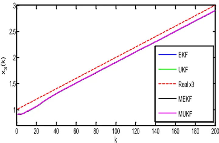
proposed MUKF. Simulation was repeated 100 times. For state variable

𝑥

, simulation results are

given in Figures 1-2 and the mean square errors (MSE) of all variables are given Table 2 and Table

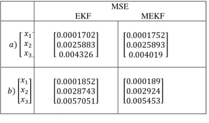
3. As, it can be seen, for all state variables the proposed MUKF is giving better results than

conventional UKF. For state variable

𝑥

, performance of the proposed MUKF is the best,

performance of the MEKF is better than EKF and UKF. But for state variables

𝑥

and 𝑥

, the EKF

demonstrates the best performance.

5.

CONCLUSION

In this paper, with the intention to improve the performance of the UKF for special

nonlinear signal models, MUKF algorithm is introduced. The MUKF contains two parallel

algorithms. Algorithm I is used for yielding the estimates which are used in Algorithm II

to implement conventional Kalman Filter Algorithm. Two algorithms are applied in parallel

starting with the same initial estimate.

In simulation study, a nonlinear system that contains a linear subsystem is

considered. EKF, MEKF, UKF and newly proposal MUKF were applied to obtain systems

states estimates and results are compared using mean square error criteria.

ESIN KOKSAL BABACAN, MILOS I. DOROSLOVACKI AND LEVENT ÖZBEK

It can be seen that, performance of the proposed MUKF is better than UKF in

terms of mean square estimation error. As a result, we can say that the proposed MUKF is

considered as an alternative method to parameter estimation problem in state-space models.

Table 2. MSE of EKF and MEKF

MSE

EKF MEKF

𝑎) [

𝑥

𝑥

𝑥

]

[

0.0001702

0.0025883

0.004326

]

[

0.0001752

0.0025893

0.004019

]

𝑏) [

𝑥

𝑥

𝑥

]

[

0.0001852

0.0028743

0.0057051

]

[

0.000189

0.002924

0.005453

]

Table 3. MSE of UKF and MUKF

MSE

UKF MUKF

𝑎) [

𝑥

𝑥

𝑥

]

[

0.0001822

0.0026913

0.004229

]

[

0.0001752

0.0025633

0.003973

]

𝑏) [

𝑥

𝑥

𝑥

]

[

0.000205

0.003013

0.005513

]

[

0.0001882

0.0028963

0.005344

]

Figure 1. Estimation of state variable 𝑥

(𝑘) for case a

Figure 2. Estimation of state variable 𝑥

(𝑘) for case b

6.

REFERENCES

[1] K. Xiong, H. Zhang and C.W. Chan, “Performance Evaluation UKF- Based Nonlinear Filtering”,

Automatica, Elsevier, 42 (2), pp. 261-270, 2006.

[2] K.H. Kim, J.G. Lee, C.G. Park and G.I. Jee, “The Stability Analysis of the Adaptive Fading

Kalman Filter”, 16 th IEEE International Conference on Control Applications, IEEE, Singapore,

pp. 982-987, 1-3 October 2007.

0

20

40

60

80

100

120

140

160

180

200

0.9

0.95

1

1.05

1.1

k

EKF

UKF

Real x3

MEKF

MUKF

0 20 40 60 80 100 120 140 160 180 200 1 1.5 2 2.5 3

k

ESIN KOKSAL BABACAN, MILOS I. DOROSLOVACKI AND LEVENT ÖZBEK

[3] S.J. Julier, J.K. Uhlmann and H.F. Durratnt-Whyte, “A new Approach for Filtering Nonlinear

system”. Proceedings of American Control Conference, pp. 1628-1632, Washington, DC, 1995.

[4] S.J. Julier and J.K. Uhlmann, “A New Extension of the Kalman Filter to Nonlinear Systems”,

Int.

Symp. Aerospace/Defense Sensing, Simul. and Controls,

Orlando, FL, SPIE, doi:

10.1117/12.280797, pp. 182-193, 21–24 April 1997.

[5] S.J. Julier and J. Uhlmann, “The Scaled Unscented Transformation”, American Control

Conference, IEEE, Anchorage, pp. 4555-4559, 2002.

[6] B. Ristic, A. Farina, D. Benvenuti and M.S. Arulampalam. “Performance Bounds and

Comparision of Nonlinear Filters for Tracking a Ballistic Object on Re-entry”, IEEE proceedings

of the radar Sonar Navigation, 150 (2), pp. 65-70, 2003.

[7] Wan, E. A. and Van der Merwe, R. (2000). “The Unscented Kalman Filter for Nonlinear

Estimation”,. Adaptive Systems for signal processing, Communications and Control Symposium,

IEEE, pp. 153-158, 1-4 October 2000.

[8] C. Chui, G. Chen and H.C. Chui, “Modified Extended Kalman Filtering and a Real-Time Parallel

Algorithm for System Parameter Identification”, IEEE, Transactions on Automatic Control, 35

(1), pp. 100-104, January 1990.

[9] K. Xiong, L.D. Liu and H.Y. Zhang. “Modified Unscented Kalman Filtering and its Application

in Autonomous Satellite Navigation”, Aerospace Science and Tecnology, Elsevier, 13 (4), pp.

238-246, 2009.

Current Address: Esin Köksal Babacan, Ankara University, Department of Statistics, Faculty of Science, 06100 Tandoğan, Ankara-TURKEY

E-Mail: ekoksal@science.ankara.edu.tr

Current Address: Miloš I. Doroslovački, The George Washington University, Department of Electrical and Computer Engineering Washington, DC 20052, USA

E-Mail: doroslov@gwu.edu

Current Address: Levent Özbek, Ankara University, Department of Statistics, Faculty of Science, 06100 Tandoğan, Ankara-TURKEY