Color science and technology of novel nanophosphors for high-efficiency high-quality LEDs

(1)

COLOR SCIENCE AND TECHNOLOGY OF

NOVEL NANOPHOSPHORS FOR

HIGH-EFFICIENCY HIGH-QUALITY LEDs

A THESIS

SUBMITTED TO THE DEPARTMENT OF ELECTRICAL AND ELECTRONICS ENGINEERING

AND THE GRADUATE SCHOOL OF ENGINEERING AND SCIENCE OF BILKENT UNIVERSITY

IN PARTIAL FULLFILMENT OF THE REQUIREMENTS FOR THE DEGREE OF

MASTER OF SCIENCE

By

Talha Erdem

August 2011

(2)

I certify that I have read this thesis and that in my opinion it is fully adequate, in scope and in quality, as a thesis for the degree of Master of Science.

Assoc. Prof. Dr. Hilmi Volkan Demir (Supervisor)

Prof. Dr. Ayhan Altıntaş

Assoc. Prof. Dr. Dönüş Tuncel

Approved for the Graduate School of Engineering and Science:

Prof. Dr. Levent Onural

(3)

ABSTRACT

COLOR SCIENCE AND TECHNOLOGY OF

NOVEL NANOPHOSPHORS FOR HIGH-EFFICIENCY

HIGH-QUALITY LEDs

Talha Erdem

M.S. in Electrical and Electronics Engineering

Supervisor: Assoc. Prof. Dr. Hilmi Volkan Demir

August 2011

Today almost one-fifth of the world‟s electrical energy is consumed for artificial lighting. To revolutionize general lighting to reduce its energy consumption, high-efficiency, high-quality light-emitting diodes (LEDs) are necessary. However, to achieve the targeted energy efficiency, present technologies have important drawbacks. For example, phosphor-based LEDs suffer from the emission tail of red phosphors towards longer wavelengths. This deep-red emission decreases substantially the luminous efficiency of optical radiation. Additionally, the emission spectrum of phosphor powders cannot be controlled properly for high-quality lighting, as this requires careful spectral tuning. At this point, new nanophosphors made of colloidal quantum dots and crosslinkable conjugated polymer nanoparticles have risen among the most promising alternative color convertors because they allow for an excellent capability of spectral tuning. In this thesis, we propose and present efficiency, high-quality white LEDs using quantum dot nanophosphors that that exhibit luminous efficacy of optical radiation ≥380 lm/Wopt, color rendering index ≥90 and

correlated color temperature ≤4000 K. We find that Stoke‟s shift causes a fundamental loss >15%, which limits the maximum feasible luminous efficiency to 326.6 lm/Welect. Considering a state-of-the-art blue LED (with 81.3% photon

(4)

200 lm/Welect, the layered quantum dot films are required to have respective

quantum efficiencies of 39 and 79%. In addition, we report our numerical modeling and experimental demonstrations of the quantum dot integrated LEDs for the different vision regimes of human eye. Finally, we present LEDs based on the color tuning capability of conjugated polymer nanoparticles for the first time. Considering the outcomes of this thesis, we believe that our research efforts will help the development and industrialization of white light emitting diodes using nanophosphor components.

Keywords: White light emitting diodes (white LED), color science, photometry,

luminous efficacy, color rendering, color temperature, color tuning, spectral tuning.

(5)

ÖZET

NANOFOSFORLARIN YÜKSEK VERİMLİLİK YÜKSEK

KALİTE LED UYGULAMALARI İÇİN RENK BİLİMİ VE

TEKNOLOJİSİ

Talha Erdem

Elektrik ve Elektronik Mühendisliği Bölümü Yüksek Lisans

Tez Yöneticisi: Doç. Dr. Hilmi Volkan Demir

Ağustos 2011

Günümüzde dünya enerji tüketiminin yaklaşık beşte biri yapay aydınlatma için kullanılmaktadır. Genel aydınlatma uygulamalarında bu enerji tüketimini düşürecek teknolojik devrimi hayata geçirebilmek için verimliliği ve kalitesi yüksek ışık yayan diyotların (LED) kullanımına geçilmesi bir zorunluluk haline gelmiştir. Ancak hedeflenen verimlilik seviyelerine ulaşabilmek için günümüz teknolojilerinin önemli zaafları vardır. Örneğin, fosfor tabanlı LED‟lerin en büyük sorunları arasında kırmızı fosforların uzun dalgaboylarına uzanan ışıma spektrumları yer almaktadır. Bu derin-kırmızı bölgedeki ışıma, optik ışımanın aydınlatma verimliliğini (LER) önemli düzeyde azaltmaktadır. Bunlara ek olarak, fosfor tozlarının ışıma spektrumlarının kontrol edilemeyişi dikkatli spektrum ayarlanabilirliğini gerektiren yüksek kaliteli aydınlatma uygulamaları için sorun teşkil etmektedir. Bu noktada, kolloid kuantum noktacıkları ve çapraz zincirlenebilir polimer nanoparçacıklar spektrum kontrolüne izin vermelerinden dolayı var olan renk dönüştürücü malzemelere alternatif olarak öne çıkmaktadırlar. Bu tezde kuantum noktacık nanofosforlar kullanarak yüksek verimlilikte ve kalitede beyaz LED‟leri teklif ediyor ve gösterimini yapıyoruz. Bu LED‟lerin optik ışımanın aydınlatma verimliliği değerleri 380 lm/Wopt‟den,

renk dönüşüm indisleri ise 90‟dan daha yüksek değerlere ulaşabilmekte; benzer renk sıcaklığı ise 4000 K‟in altında yer almaktadır. Sadece Stock kaymasından

(6)

kaynaklanan temel kaybın en az %15 olduğunu ve elektriksel aydınlatma verimliliğinin (LE) en yüksek 326.6 lm/Welect olabileceğini yine bu tezde

gösteriyoruz. Bu da güç dönüşüm verimliliği açısından günümüzün en iyi mavi LED‟leri kullanıldığında (%81.3), 265.5 lm/Welect seviyesinde bir elektriksel

aydınlatma verimliğine denk gelmektedir. 100 ve 200 lm/Welect seviyesine

ulaşmak için katmanlı kuantum noktacık filmlerinin verimliliklerinin sırasıyla %39 ve %79 olması gerekmektedir. Bu iç aydınlatma uygulamaları için yapılan çalışmaların yanında, diğer görme modları için de modelleme ve deneysel gösterimlerimiz yine bu tez içerisinde yer almaktadır. Son olarak, renk kontrolüne imkân veren konjüge edilmiş polimer nanoparçacıkların da ilk defa bir LED tasarımında kullanımını rapor ediyoruz. Bu tezdeki çalışmalarımızı göz önüne alarak, çalışmalarımızın nanofosfor temelli beyaz LED‟lerin geliştirilmesi ve endüstrileşmesinde önemli katkıları olacağını ummaktayız.

Anahtar Kelimeler: Beyaz ışık yayan diyotlar (beyaz LED), renk bilimi,

aydınlatma verimliliği, renk dönüşümü, renk sıcaklığı, renk kontrolü, spektrum kontrolü.

(7)

Acknowledgements

“Bihî, the word that adorns every other word…”

As one of the major milestones of my life, herewith I finished my MS studies with this thesis. There have been a lot of people who helped and supported me during this process, which had been sometimes very stressful and sometimes very entertaining. I owe many thanks to all of them.

First, I would like to thank my supervisor Prof. Hilmi Volkan Demir. He helped and supported me in every part of this thesis; more importantly, he has been always very kind and friendly to me. I would also like to thank Prof. Dönüş Tuncel, who has guided and helped me during our collaborative works. I owe many thanks to Prof. Ayhan Altıntaş, who has accepted to be in my thesis committee.

Dr. Sedat Nizamoglu and Evren Mutlugün have never hesitated to help me. More importantly, they have been great guides in my research as well as great friends of mine. Their friendship will never be forgotten.

I would also like to thank all the past and present members of Demir Group: Emre Sarı, Tuncay Özel, Rohat Melik, İlkem Özge Özel, Aslı Yılmaz, Gülis Zengin, Neslihan Çiçek, Refik Sina Toru, Can Uran, Cüneyt Eroğlu, Onur Akın, Kazım Gürkan Polat, Mustafa Akın Sefünç, Burak Güzeltürk, Hatice Ertuğrul, Sayım Gökyar, Veli Tayfun Kılıç, Kıvanç Güngör, Ahmet Fatih Cihan, Shahab Akhavan, Yusuf Keleştemur, Yasemin Coşkun, Durmuş Uğur Karatay, Ozan Yerli, Togay Amirahmadov, Özgün Akyüz, Dr. Nihan Koşku Perkgöz, Dr. Urartu Özgür Ş. Şeker, Dr. Pedro Ludwig Hernandez-Martinez, Dr. Olga Samarskaya. It is/has been a privilege working with all these people.

(8)

During my master‟s studies, I worked closely with the Dönüş Tuncel‟s Group. In addition to the many skills that I gained during my research with them, I also had great friends. Knowing all of them has been a great honor for me. I would like to thank Dr. Eun Ju Park, Zeynep Göksel Özsarp, Müge Artar and Vüsala Ibrahimova for their excellent friendship. I enjoyed every minute of it while working with them.

In addition to all these great people, I also would like to thank Dr. Stephen Hickey and Dr. Nikolay Gaponik for their hospitality while I was in Dresden. At this point, I, of course, thank my family: My father and mother, for their supports and patience, and for many things that I cannot put into words. Also I owe many thanks to my brothers that are with me whenever I need them. I would also like to thank my aunt and her husband, who have turned Ankara to a bearable city for me.

(9)

List of Figures

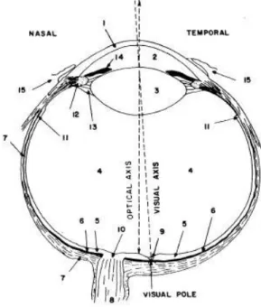
Figure 2.1 Structure of the human (right) eye. (1) cornea, (2) aqueous humor, (3) lens, (4)vitreous body, (5) retina, (6) choroid, (7) sclera, (8) optic nerves, (9) fovea, (10) optic disk, (11) front edge of retina, (12) ciliary muscle, (13)

zonule fibers, (14) iris and (15) ocular conjunctiva [7]. ... 5

Figure 2.2 Rod and cone receptors in the eye [10]. ... 6

Figure 2.3 Normalized spectral sensitivities of rods and cones (red, green and blue) [9]. ... 6

Figure 2.4 Color matching functions as defined in CIE 1931 [11]. ... 7

Figure 2.5 CIE 1931 (x,y) chromaticity diagram [12]. ... 8

Figure 2.6 CIE 1976 chromaticity diagram [9]. ... 9

Figure 2.7 Planckian locus on CIE 1976 (u',v') chromaticity diagram [9]. ... 16

Figure 2.8 The eye sensitivity function at different vision regimes: Photopic (red), mesopic (green, at a luminance of 0.5 cd/m2 ) and scotopic eye sensitivity functions. ... 17

Figure 3.1 Semiconductor QDs. (a) Colloidal semiconductor CdTe QDs in dispersion. (b) Epitaxially grown InAs QDs within a GaAs matrix which has a larger bandgap [32]. ... 24

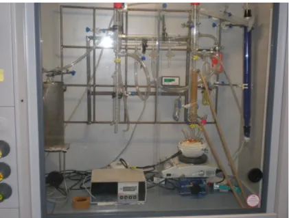
Figure 3.2 Synthesis setup of CdSe quantum dots. ... 28

Figure 3.3 CdSe quantum dots synthesized in Demir lab at UNAM. ... 29

Figure 3.4 Synthesis setup of CdTe quantum dots. ... 31

Figure 3.5 Absorption spectra of CdSe QDs having different sizes [57]. ... 33

Figure 3.6 SEM image of conjugated polymer nanoparticles of poly[(9,9-dihexylfluorene)-co-alt-(9,9-bis(3-azidopropyl)fluorene)] (PF3A) which are crosslinked for three hours [63]. ... 36

(12)

Figure 5.1 CRI vs. LER dependence between (a) 2450 K<CCT<2550 K, (b) 2950 K<CCT<3050 K, and (c) 3450 K<CCT<3550 K. ... 46 Figure 5.2 Relations between (a) CRI and CCT, (b) CRI and LER, and (c) LER

and CCT. ... 47 Figure 5.3 (a) CRI vs. LER relationship and (b) LER vs. CCT relationship for

white data points (shown in red) and near-white points (shown in blue). .. 48 Figure 5.4 The relative spectral power distribution for the average values of

input parameters in the case of (a) CRI>80 and LER>300 lm/Wopt and (b)

CRI>90 and LER>380 lm/Wopt. ... 53

Figure 5.5 Potential performance of WLED designs using the combinations green, yellow and orange of QDs emitting at 528, 260 and 609 nm [93]. . 55 Figure 5.6 The emission spectra and chromaticity coordinates of WLED#1

together with the picture of the WLED [93]. ... 56 Figure 5.7 The emission spectra and chromaticity coordinates of WLED#2

together with the picture of the WLED [93]. ... 57 Figure 5.8 The emission spectra and chromaticity coordinates of WLED#3

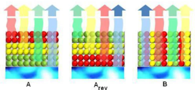
together with the picture of the WLED [93]. ... 57 Figure 5.9 Three basic architectures of QD-WLEDs modeled in this work: A,

Arev and B. ... 60

Figure 5.10 Illustration of optical mechanisms using system box model for architecture A. ... 66 Figure 5.11 Illustration of optical mechanisms using system boxes for Arev. .... 70

Figure 5.12 Illustration of optical mechanisms using system boxes for B. ... 74 Figure 5.13 Fraction of blue photons transferred to green QDs (bg), to yellow

QDs (by), to red QDs (br), and being extracted (be); fraction of green photons self-absorbed (gg), transferred to yellow QDs (gy), to red QDs (gr), and being extracted (ge); fraction of yellow photons self-absorbed (yy), transferred to red QDs (yr), and being extracted (ye); fraction of red photons self-absorbed (rr) and being extracted (re) in A and B at =100%. ... 83 Figure 5.14 Fraction of blue photons transferred to green QDs (bg), to yellow

QDs (by), to red QDs (br), and being extracted (be); fraction of green photons self-absorbed (gg), transferred to yellow QDs (gy), to red QDs (gr), and being extracted (ge); fraction of yellow photons self-absorbed

(13)

(yy), transferred to red QDs (yr), and being extracted (ye); fraction of red photons self-absorbed (rr) and being extracted (re) in A and B at =50%. 83 Figure 6.1 Relation and tradeoffs between (a) LER vs. S/P ratio, (b) CQS vs. S/P

ratio, (c) CQS vs. LER, (d) CCT vs. LER, (e) CCT vs. CQS, and (f) CCT

vs. S/P ratio. ... 92

Figure 6.2 WLED designs with input parameters modeled for CQS≥70, 80 and 90 restrictions in order. All of these WLED designs satisfy S/P ratio≥2.50 and LER≥250 lm/Wopt. ... 96

Figure 6.3 The emission spectra of the QD-WLED and corresponding

chromaticity point on CIE 1931 chromaticity diagram along with the photo of the QD-WLED [103]. ... 98 Figure 6.4 Mesopic luminance (Lmes) vs. radiance (P) for several light sources:

standard daylight source (D65), cool white fluorescent lamp (CWFL), blackbody radiator at 3000K (BR@3000K), metal-halide lamp (MH), high pressure sodium lamp (HPS) and mercury vapor lamp (MV), WLED#1, WLED#2, WLED#3. ... 102 Figure 6.5 QD-WLED spectra leading to the highest mesopic luminance (Lmes)

for standard 1 (WLED#1), standard 2 (WLED#2), and standards 3&4 (WLED#3). ... 109 Figure 7.1 Molecular structure of

poly[(9,9-dihexylfluorene)-co-alt-(9,9-bis-(3-azidopropyl)fluorene)] (PF3A) [63]. ... 112 Figure 7.2 Photoluminescence graphs of PF3A-L nanoparticles crosslinked (a)

in air and (b) under nitrogen atmosphere for varying durations between 1 and 6 hours [63]. ... 113 Figure 7.3 Photoluminescence graphs of PF3A-S nanoparticles crosslinked (a) in

air and (b) under nitrogen atmosphere for varying durations between 1 and 6 hours [63]. ... 113 Figure 7.4 Photoluminescence spectra of the films prepared using (a) PF3A-L

NP and (b) PF3A-S NP dispersions that are not crosslinked and crosslinked for 3 hours in air and under nitrogen [63]. ... 115 Figure 7.5 Electroluminescence spectrum of the final device where PF3A-S

(14)

List of Tables

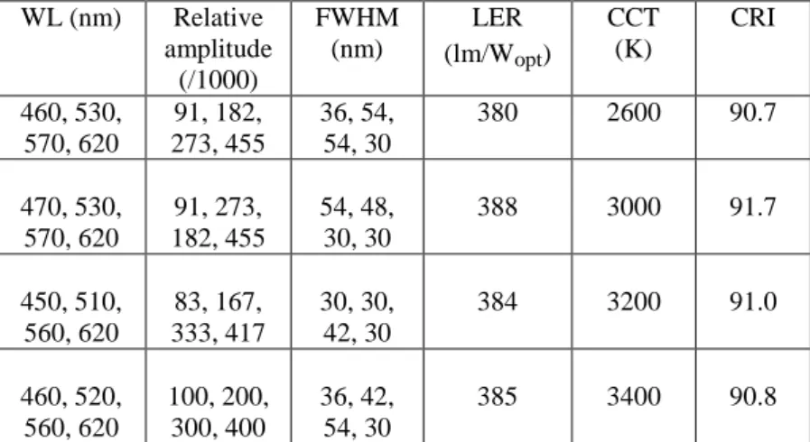
Table 5.1 Average and standard deviation values of the input parameters of the spectra satisfying the conditions of CRI>80 and LER>300 lm/Wopt, and

CRI>90 and LER>380 lm/Wopt. ... 50

Table 5.2 Exemplary results of the photometric computations. In the columns of WL, relative amplitude, and FWHM, the first numbers belong to the corresponding property of the blue spectrum. The other numbers in those columns stand for green, yellow, and red spectral content, respectively. .. 52 Table 5.3 Maximum, minimum, average and standard deviation of PCE

(excluding PCE of blue LED) and LE (including PCE of blue LED) for the photometrically efficient spectra. ... 80 Table 5.4 Maximum, minimum, average and standard deviation of LE

(including PCE of blue LED) in lm/Welect for the photometrically efficient

spectra at QD‟s = 80%, 50% and 20% for two different architectures: A and B. The effect of self-absorption (SA) is also investigated for

architecture A. ... 81 Table 5.5 Maximum, minimum, average and standard deviation of PCE

(excluding PCE of blue LED) in percentages for the photometrically efficient spectra at = 80%, 50% and 20% for two different architectures. The effect of self-absorption (SA) is also investigated for architecture A. 81 Table 5.6 Average of the spectral parameters belonging to the spectra whose

PCE is larger than the average of the PCEs of the photometrically efficient spectra in A and B at varying quantum efficiencies. i: peak emission

wavelength, Δ i: full-width at half-maximum, ai: weight of the color

component i. i is either blue (b), green (g), yellow (y) or red (r). ... 84 Table 6.1 Average and standard deviation of the input parameters satisfying the

conditions S/P ratio≥2.50, LER≥250 lm/Wopt and CQS≥70, 80 and 90. ... 93

Table 6.2 Spectral parameters resulting in the highest Lmes for all the four

standards used. : peak emission wavelength, : FWHM and a:

amplitudes of color components of blue, green, yellow and red. ... 103 Table 6.3 Average and stdev of Lmes, CQS, CCT for QD-WLED designs ... 103

(15)

Table 6.4 Average and stdev of spectral parameters for all four standards studied here. : peak emission wavelength, : FWHM and a: amplitudes of color components of blue, green, yellow and red. ... 103 Table 7.1 Photometric computation results of PF3A-L dispersions for different

cross-linking durations [63]. ... 114 Table 7.2 Photometric calculation results of PF3A-S dispersions at different

crosslink durations [63]. ... 114 Table 7.3 Results of the photometric calculations carried out on the

(16)

Chapter 1 Introduction

Today traditional fossil based energy production undesirably leads to dramatic increase in CO2 content of the atmosphere, which consequently adversely affects

the climate [1]. To slow down this trend, scientists throughout the world continue working on energy efficiency in different fields of science [2,3]. One of those areas is the reduction and optimization of the energy consumed by the electrical devices, which can take a significant role in combatting climate change if targeted performance levels are realized.

Among various applications, lighting has an important place for potential energy saving as today ca. 20% of the global electrical energy consumption is used for the artificial lighting [4]. In the under-developed parts of the world, gas lamps are still used, which possess very low light quality and efficiency. As the regional economic power increases, the most widely used light sources become fluorescent lamps (and incandescent lamps in some places). However, these sources are not enough for high-efficiency.

Solid state lighting offers a huge potential in terms of energy efficiency. If the light emitting diodes (LED) achieve the targeted efficiencies, the energy consumed for lighting applications can be reduced by fifty percent [5]. According to a recent report published by the US Department of Energy, 133 TWh of electrical energy can be saved annually in the USA in case that general illumination sources are replaced entirely with LEDs [6]. However, to realize such a large-scale change of light sources, they need to be designed specifically

(17)

for the aimed applications so that high-quality white light can be obtained in addition to high-efficiency, requiring a reasonable production cost and capacity.

For high-quality lighting, the capability of the light sources to render the real colors of the illuminated objects is an important criterion. In addition to increasing the life quality, especially for indoor lighting, this property of light sources can be crucial for street lighting applications since good color rendering increases the perception of color contrast under low ambient lighting conditions, which consequently might help to save human life against the risk of life-threatening accidents. Moreover, a good light source should have a good spectral match between the emitted light spectrum and the human eye sensitivity function at the luminance levels of the specific applications. If this spectral match is not good enough, the emitted optical power by the device cannot be efficiently perceived by the human eye. Furthermore, a warm white shade is desirable especially for indoor lighting applications as it can otherwise affect the human biological clock.

Satisfying all of these high-quality lighting requirements simultaneously, in addition to high energy efficiency, requires careful spectral design and material choice. Conventional light sources such as incandescent and fluorescent lamps cannot fulfill these needs as their efficiencies are not high enough and/or tuning their spectra is not possible. Although power conversion efficiencies of white LEDs, in which phosphors are typically integrated as color convertors, are relatively good, their spectra cannot be controlled and tuned to the desired extent. As a result, they fail in satisfying the requirements for high-quality white light stated above. Spectral tuning can be achieved when individual LED chips emitting different color components are used together. However, this requires an individual green-emitting LED, which is low efficiency. Also, this multichip approach for spectrally tunable white light generation is far from being cost effective.

(18)

One of the candidate materials, which can be used for color conversion instead of conventional phosphors on blue (or UV) LED chips and allows spectral tuning, is the colloidal semiconductor quantum dots (QDs). Since their emission properties can be fine-tuned by controlling their sizes and monodispersity, using multiple color components with individual narrow emission bands around strategic wavelengths enables to obtain a white light satisfying the requirements aforementioned. Another class of materials, whose emission spectra can also be tuned, is the conjugated polymer nanoparticles. By crosslinking and building a core-shell type of nanoparticle structure, one can tune the photoluminescence spectra of these particles. As a result, spectral requirements for some specific applications can be satisfied using these nanoparticles as color convertors on LED chips emitting at shorter wavelengths.

This thesis presents the results of the thesis research work for obtaining efficient, high-quality and application specific white LED designs using colloidal quantum dots and conjugated polymer nanoparticles. It is organized as follows: Chapter 1 provides a general introduction and overview to the problems addressed in our research. In Chapter 2, the basic background regarding color science and photometry is given, which is useful for evaluating the quality of the generated light in a quantitative basis. Chapter 3 covers the optical properties of the materials used in this thesis work, i.e., quantum dots and polymer nanoparticles. Chapter 4 is dedicated to the white light generation methods using LEDs. Our studies on quantum dot integrated white LEDs for indoor lighting applications are explained in Chapter 5. The performance of quantum dot integrated white LEDs for outdoor applications is discussed in Chapter 6. Chapter 7 summarizes our work on white light generation using conjugated polymer nanoparticles via crosslinking. Finally, in Chapter 8 we summarize our conclusions of this thesis.

(19)

Chapter 2 Color Science and Photometry

To evaluate the quality of white light sources, one needs to have quantitative measures so that light sources can be classified accordingly. For this purpose, basic information on color science and photometry is essential. In this chapter, we review these points starting from the structure of a human eye. Then we continue with discussing the color matching functions and color spaces. Following these, two important color rendering metrics, i.e., color rendering index and color quality scale, are explained. Subsequently, we move to the photometry and start with the eye sensitivity functions for different vision regimes and continue with the definitions of some basic photometric quantities. Then we explain luminous efficacy of optical radiation and luminous efficiency of the light sources. Finally we close this chapter with the description of scotopic-to-photopic ratio (S/P ratio) and mesopic luminance.

2.1 The Structure of Human Eye

The eye is the organ through which we see our environment. Therefore, understanding its structure and working is essential for the purposes of high-quality light generation. It has an almost spherical shape with a diameter of ca. 24 mm [7]. The cornea is the layer of the eye where the light rays first enter (Figure 2.1). It is a transparent structure and contains no blood vessels. In its front part, it exhibits an additional curvature, whose radius of curvature is about 8 mm. Tears and mucus solutions help the eye to sustain its transparency. After cornea, the light rays pass through the so-called anterior chamber which is full of a transparent liquid known as aqueous humor controlling the pressure within the eyeball. As the interior pressure of the eye is greater than the atmospheric

(20)

pressure, the amount of this liquid is essential for protecting the shape of the eye. Following this liquid part, light rays come to the lens which is responsible for focusing the incoming rays on the retina. The position of the focus is controlled through the shape change of the lens by two muscles. These muscles pull or relax the lens when the eye focuses on a far or close object and the lens takes a flat or convex shape, respectively. After the lens, light rays travel within the vitreous body, which is filled by a jelly material, and fall on the retina. This part of the eye corresponds to the two-thirds of the volume of the eye.

Figure 2.1 Structure of a human (right) eye. (1) cornea, (2) aqueous humor, (3) lens, (4)vitreous body, (5) retina, (6) choroid, (7) sclera, (8) optic nerves, (9) fovea, (10) optic disk, (11) front edge of retina, (12) ciliary muscle, (13) zonule fibers, (14) iris and (15) ocular conjunctiva [7].

The retina is the part of the eye where the most critical layers for vision are located and neurons and fibers are contained. According to Stell, the neurons constitute three main layers [8]. The first layer is the layer of photoreceptors; the second one is the layer of intermediate neurons. Finally, the third neural layer is the layer of ganglion cells. The light sensitive cells are called photoreceptors. There are two types of them: rods and cones. The retina is rich of rods, which are more sensitive to light compared to cones. Their sensitivity covers the whole

(21)

visible range without useful color differentiation; as a result, they cannot provide color information to the brain. On the other hand; cones have three types, each having a different wavelength range of sensitivity corresponding to blue, green and red colors [9]. As Figure 2.2 illustrates, the photoreceptors are named considering their shapes. Figure 2.3 shows the relative sensitivities of rods and red, green and blue photoreceptors with respect to optical wavelength [9].

Figure 2.2 Rod and cone receptors in the eye [10].

Figure 2.3 Normalized spectral sensitivities of rods and cones (red, green and blue) [9].

In addition to their spectral sensitivities, the photoreceptor activity depends on the ambient lighting levels. At high light levels, cones are more active and they dominate the vision whereas rods saturate and do not have any significant contribution to the vision. The vision at this light level is called the photopic vision. On the other hand, cones are not sensitive enough at lower light levels while rods dominate the vision. This is why we cannot distinguish different colors in the dark. This vision regime is called scotopic. There is another vision

(22)

regime where rods and cones are both active and contribute to the vision simultaneously. This regime is called the mesopic vision whose limits and significance will be discussed in the further sections of this chapter.

2.2 Color Matching Functions and Color Spaces

To engineer light sources, one needs to define colors in a mathematical sense. However, color perception of every individual slightly varies; therefore, such a definition has to be made using a statistical approach. The International Commission for Illumination (Commission Internationale de l‟Eclairage, CIE) has used such an approach and published a standardized method for the definition of color [11]. CIE utilized three color matching functions: x, y and z, whose spectral distributions are given in Figure 2.4.

Figure 2.4 Color matching functions as defined in CIE 1931 [11].

The method proposed by CIE makes use of these color matching functions and the chromaticity diagram. The tristimulus values, X, Y and Z, are given in Equations (2.1) – (2.3) for a spectral power distribution of s(λ).

(23)

( ) ( ) X s x d (2.1) ( ) ( ) Y s y d (2.2) ( ) ( ) Z s z d (2.3)

The chromaticity coordinates are calculated as in Equations (2.4) – (2.7). The chromaticity diagram, which is created by using the mapping methodology described in Equations (2.1) – (2.6), is given in Figure 2.5. Since one of the three coordinates is dependent on the other two, a two dimensional color space is enough without having any information loss.

X x X Y Z (2.4) Y y X Y Z (2.5) 1 Z z x y X Y Z (2.6)

Figure 2.5 CIE 1931 (x,y) chromaticity diagram [12].

Although CIE 1931 is the most widely used chromaticity diagram, it has some important weaknesses, which was later improved by defining new color

(24)

spaces. One of the important drawbacks of CIE 1931 is that the geometric difference between colors does not correspond to the same color differences. To fix this problem, CIE introduced new chromaticity diagrams in 1960 and 1976, which are called CIE 1960 and 1976 chromaticity diagrams, respectively. These diagrams are also called (u,v) and (u',v') chromaticity diagrams [13,14]. CIE 1976 chromaticity diagram is given in Figure 2.6.

Figure 2.6 CIE 1976 chromaticity diagram [9].

Calculations of (u,v) and (u',v') chromaticity coordinates are given in Equations (2.7) – (2.9). 4 ' 15 3 X u u X Y Z (2.7) 6 15 3 Y v X Y Z (2.8) 9 ' 15 3 Y v X Y Z (2.9)

Another uniform color space is the CIE 1976 (L*a*b*) chromaticity diagram [14]. The corresponding equations required for color mapping are given by Equations (2.10) – (2.12) [7].

(25)

* 1/3 116( / _n) 16 L Y Y (2.10) 1/3 1/3 * 500 n n X Y a X Y (2.11) 1/3 1/3 * 200 n n X Z b X Z (2.12)

These formulas are valid as long as X/Xn, Y/Yn and Z/Zn are larger than 0.01.

Otherwise the calculations should be carried out using Equations (2.13) – (2.17). * 903.3 m n Y L Y (2.13) * 500 m n n X Y a f f X Y (2.14) * 200 m n n X Z b f f X Z (2.15) where 1/3 0.008856 n n n K K K f for K K K (2.16) 16 7.787 0.008856 116 n n n K K K f for K K K (2.17)

for K is X, Y or Z. Xn, Yn and Zn are called the nominally white object color

stimulus, and they are calculated by making use of the spectral power distributions of CIE standard illuminants like A and D65 and Equations (2.1) –

(26)

2.3 Color Rendering Index and Color Quality

Scale

A good white light source has to render the real colors of the objects that it illuminates. It is very critical especially for the indoor lighting applications; however, for outdoor applications, it also helps to increase the safety because good color rendering provides better color contrast and consequently, better vision under low ambient lighting.

The color rendering capability of the illuminants is calculated by several methods. In this thesis, we explain the most widely used two metrics i.e.: the color rendering index (CRI) and the color quality scale (CQS), which is developed as a similar approach to CRI.

The color rendering index (CRI) is developed by CIE in 1971 [15] and updated to its current form in 1995 [16]. It basically tests the color rendering capability of the test light source with respect to a reference light source, which is accepted to possess perfect color rendition. CRI makes use of fourteen test color samples suggested by CIE. Based on the reflection of the test light source and the reference light source from these samples, color differences are calculated for each test sample. Finally, from these color differences a color rendering index value specific for each sample is obtained. The first eight of these samples are used for determining the general color rendering index. The remaining six define the special color rendering indices. The best color rendition is given as 100, whereas the worst rendition is denoted by a CRI of -100.

Before explaining the calculation of CRI, it is helpful to clarify the notation. The subscript “ref” stands for the reference light source, which is in general a blackbody radiator. The subscript “ref,i” denotes the reflected color from the ith

(27)

test sample illuminated by the reference light source. The subscript “test” indicates for the light source under the test whereas “test,i” is the reflection of the test light source from the ith test samples.

The calculation starts with the transformation of (u,v) coordinates to (c,d) coordinates given by Equations (2.18) and (2.19).

(4 10 ) /

c u v v (2.18)

(1.708 0.404 1.481 ) /

d v u v (2.19)

Then (utest,i**,vtest,i**) are calculated by Equations (2.20) and (2.21).

, , ** , , , 10.872 0.404 4 16.518 1.481 ref ref test i test i test test test i ref ref test i test i test test c d c d c d u c d c d c d (2.20) ** , , , 5.520 16.518 1.481 test i ref ref test i test i test test v c d c d c d (2.21)

The calculation of (utest**,vtest**) is given in Equations (2.22) and (2.23).

** 10.872 0.404 4 16.518 1.481 ref ref test ref ref c d u c d (2.22) ** 5.520 16.518 1.481 test ref ref v c d (2.23)

For the calculation of color shift, we need ΔL**_{, Δu}**

and Δv** (Equations (2.24) – (2.27)).

1/3 1/3

** ** **

, , , ,

25 _{ref i} 17 25 _{test i} 17 _{ref i} _{test i}

L Y Y L L (2.24)

** ** ** ** **

, , , ,

13 _{ref i}( _{ref i} _ref) 13 _{test i}( _{test i} _test)

u L u u L u u (2.25)

** ** ** ** **

, , , ,

13 _{ref i}( _{ref i} _ref) 13 _{test i}( _{test i} _test)

v L v v L v v (2.26)

Following these, the color difference is calculated as in Equation (2.27).

** ** 2 ** 2 ** 2

( ) ( ) ( )

i

(28)

After obtaining the color difference, individual color rendering indices of each test color sample can be obtained using Equation (2.28).

*

100 4.6

i i

CRI E (2.28)

Finally, the general color rendering index is obtained by taking the average of the first eight test color samples (Equation 2.29).

8

1

8 i i

CRI CRI (2.29)

Although CRI is still the most frequently used metric for color rendition, it suffers from some weaknesses that need to be overcome [17]. One of these problems is the uniform color space used in CRI, which is not recommended by CIE anymore. Another important issue regarding CRI is that it assumes perfect color rendering of blackbody radiators and reference sources even at very low and high correlated color temperatures (CCT, which will be explained in the next section). However, this is not always correct. Furthermore, CRI does not use any test color sample, which is highly saturated. As a result, it does not provide correct color rendering information of saturated colors although the results are accurate for samples having desaturated colors. On top of these, CRI makes use of the arithmetic mean of color rendering indices of each test color sample, which means that a poor rendering for one of the samples can be compensated.

Considering these problems of CRI, Davis and Ohno have developed a new metric for color rendition evaluation of light sources called color quality scale (CQS) [17]. It uses the same reference light sources as in CRI, but the test color samples are changed. Instead of eight unsaturated test color samples, CQS employs fifteen commercially available Munsell samples, all having highly saturated colors. Since a light source rendering saturated colors well succeeds a good rendition of unsaturated colors, this metric provides more healthy information of color rendering. This is especially useful for light emitting diodes, which are fabricated using narrow-band emitting material systems and structures. As it is done in the calculation of CRI, a chromatic adaptation

(29)

transform is necessary in CQS. However, CQS utilizes a modern transform, CMCCAT2000 [18]. Another important improvement of CQS compared to CRI is the choice of uniform color space. In CQS, CIE L*a*b* is preferred. The color difference between the reflections of the test samples illuminated by the reference and test light source is expressed in Equation (2.30).

* * 2 * 2 * 2 , ( ) ( ) ( ) ab i i i i E L a b (2.30) where * * * , , i test i ref i L L L (2.31) * * * , , i test i ref i a a a (2.32) * * * , , i test i ref i b b b (2.33)

The chroma difference is given by Equation (2.34).

* * * , , , , , ab i ab test i ab ref i C C C (2.34) where * * 2 * 2 , ( ,) ( ,)

ref i ref i ref i

C a b (2.35)

* * 2 * 2

, ( ,) ( ,)

test i test i test i

C a b (2.36)

In addition to the color difference in Equation (2.30), a saturation factor is introduced in CQS so that the effect of increasing the object chroma under the test illuminant with respect to reference source is neutralized. The corrected color difference then becomes as given in Equation (2.37).

* * , , * , , _* ₂ _* ₂ , , , 0 ( ) ( ) , ab i ab i ab sat i ab i ab i E if C E E C otherwise (2.37)

One of the most important improvements of CQS compared to CRI is in the calculation of the final color rendering performance. As opposed to CRI, CQS takes root-mean-squares (rms) of individual corrected color differences, so that poor rendition of any test color sample has a more significant effect on the final value. The calculation of rms-color difference and rms-averaged CQS is given in Equations (2.38) and (2.39).

(30)

15 * 2 , , 1 1 ( ) 15 rms ab sat i i E E (2.38) , 100 3.1 a rms rms Q E (2.39)

An additional difference of CQS compared to CRI is its scale. Since having a CRI less than zero, which denotes a poor color rendition, can be misleading, CQS is brought to the scale of 0–100. This scaling is undertaken using Equation (2.40). , 0 100 10ln{exp( ) 1} 10 a rms Q CQS (2.40)

Finally, the correction for low CCTs is introduced (in Equations (2.41) and (2.42)) and the final value of CQS is determined using Equation (2.43).

For CCT < 3500 K, 3 11 2 7 (9.2672 10 ) (8.3959 10 ) (0.00255) 1.612 CCT M CCT CCT CCT (2.41) For CCT ≥ 3500 K, M_CCT 1 (2.42) 0 100 CCT CQS M CQS (2.43)

2.4 Correlated Color Temperature

The correlated color temperature (CCT) is one of the most widely used metrics for characterizing white light sources. Before defining CCT, it is more instructive first to explain the color temperature. If the chromaticity coordinates of the white light source fall onto the Planckian locus (chromaticity coordinates of blackbody radiators at different temperatures), then the temperature of the blackbody radiator having the same chromaticity points as the white light source is called the color temperature. In case that the chromaticity coordinates of the light source under test is not on the Planckian locus, then the temperature of the blackbody radiator, whose (u',v') chromaticity coordinates are closest to the light

(31)

source under the test source, is called the correlated color temperature. The Planckian locus is given in Figure 2.7.

Figure 2.7 Planckian locus on CIE 1976 (u',v') chromaticity diagram [9].

White light sources having high CCTs have a bluish shade, whereas a reddish shade corresponds to lower CCTs. Therefore, cold (or cool) white light has a higher CCT and warm white sources have lower CCTs, which might look confusing at the first sight since the use of the terminology is opposite to the common usage of temperature. An incandescent light bulb has a CCT below 3000 K, the fluorescent tubes have varying CCTs between 3000 to 6500 K whereas the CCT of the sun is close to 6000 K [9]. For indoor lighting, warm white light sources are preferred as a cool white has a high bluish content which might cause shifts in the biological clock [19].

(32)

2.5 Eye Sensitivity Functions

While evaluating the quality of the white light sources, it is of significant importance that the spectra of the illuminants match the sensitivity of the human eye as well as possible. A light source would that radiates at wavelengths not sensible by the eye cannot contribute to the vision even if it has a high power conversion efficiency or high optical power.

Since the photoreceptors contributing to the vision are different at different ambient light levels, the sensitivity of the eye changes accordingly. Rod photoreceptors are responsible for the scotopic vision, which is the dark-adapted vision [9]. Its sensitivity takes its maximum at 507 nm. On the other hand, cones provide the photon adapted vision and start to work above some luminance levels. The vision at these light levels is called the photopic vision (photon-adapted vision). The sensitivity of the cones makes its peak at 555 nm. The corresponding eye sensitivity functions for scotopic [20] and photopic [11] light levels are given in Figure 2.8.

(33)

Before explaining the mesopic vision levels, it is necessary to define the luminance, which we will explain again in the next section. The luminance of a light source is calculated as in Equation (2.44).

683 ( ) ( )

opt

lm

L P V d

W (2.44)

where P(λ) and V(λ) are the spectral radiance (power per unit area per solid angle) and the photopic eye sensitivity function, respectively.

In the mesopic levels both photoreceptors are active. As a result, the sensitivity of the eye changes according to the level of contribution of rods and cones. These changes are well known for a long time ago, however, the exact limits of photopic and scotopic regimes and the eye sensitivity function at mesopic levels have been a subject of discussion. For example, Osram Sylvania defines the luminance limits of photopic and scotopic vision as 0.003 and 3 cd/m2, respectively [21]. According to Johnson [22] and LeGrand [23] photopic vision starts at the luminance of 5 cd/m2, whereas Kokoschka pushes this limit further to 10 cd/m2 [24]. As IESNA (Illuminating Engineering Society of North America) puts these limits to around 0.01 cd/m2 and 3 cd/m2 [25], CIE 1978 claims the scotopic vision to start below 0.001 cd/ m2 [26]. According to unified system of photometry (USP) developed by Rea, photopic vision starts above 0.6 cd/m2 and scotopic vision starts below 0.001 cd/m2 [27]. Another recent system for mesopic photometry is developed by MOVE consortium; according to this work, mesopic vision lies between the luminances of 0.01 cd/m2 and 10 cd/m2 [28,29]. In 2010, CIE recommended a system of photometry (CIE 191:2010), which is based on USP and MOVE systems [30]. According to this most recent report, mesopic regime is defined between the luminance levels of 0.005 cd/m2 and 5 cd/m2. In this report, the eye sensitivity function is also defined and calculated as given in Equations (2.45) and (2.46).

( ) _mes( ) ( ) (1 ) '( )

M m V mV m V (2.45)

0

683 / ( ) ( ) ( )

mes mes mes

(34)

where V( ), V'( ) and Vmes( ) are the photopic, scotopic, and mesopic eye

sensitivity functions, respectively; P( ) is the spectral radiance, M(m) is a normalization constant such that Vmes( ) has the maximum value of 1, 0 is 555

nm, Lmes is the mesopic luminance, and m is a coefficient depending on visual

adaptation conditions. Further details on the calculation of mesopic eye sensitivity function can be found in Ref. 30. As an exemplary case, the eye sensitivity function at a luminance of 0.5 cd/m2 is given in Figure 2.8.

2.6 Basic Radiometric and Photometric Measures

The light sources are also sources of electromagnetic radiation. From this perspective, their performances can be evaluated with respect to their electromagnetic properties characterized by the radiometric measures. In addition to this, the light sources, especially white light sources, are subject to the sensitivity of the human eye. Therefore, these sources have to be evaluated by taking the response of the human eye into account. Scaling the radiometric units with the eye sensitivity function remedies this problem and introduces the photometric quantities.

One of the most frequently used radiometric quantities is the optical power. In the lighting community, radiant flux is alternatively used instead of optical power [9]. The photometric version of the optical power is the luminous flux and calculated using spectral radiant flux Pϕ(λ) and eye sensitivity function V(λ)

as in Equation (2.47). The unit of luminous flux is lumen (lm).

683 ( ) ( )

opt

lm

P V d

W (2.47)

Given the spectral radiant intensity PLI(λ), i.e., the optical power per unit

solid angle at varying wavelengths, the luminous intensity becomes as in Equation (2.48). The luminous intensity is given in units of lm/sr or equivalently in candelas (cd).

(35)

683 _LI( ) ( ) opt

lm

LI P V d

W (2.48)

The irradiance is the optical power per unit area, its correspondent in photometry is the illuminance which has the units of lm/m2. Given the spectral radiance (in units of Woptm-2nm-1) PIl(λ), the luminance is expressed as in

Equation (2.49). Its unit is lm/m2, or equivalently lux.

683 _Il( ) ( )

opt

lm

Il P V d

W (2.49)

Finally, the radiance is the radiometric quantity denoting the optical power per solid angle per unit area and has the units of Woptsr-1m-2. Given the spectral

radiance PL(λ), the luminance is calculated using Equation (2.50). Its unit is

lm/(m2sr), or equivalently cd/m2. 683 _L( ) ( ) opt lm L P V d W (2.50)

At this point, it is worth mentioning that the photometric quantities defined in this section are based on the photopic eye sensitivity function. However, photometric measures for mesopic and scotopic eye sensitivity functions may also be defined in the same way, but in those cases mentioning the type of the eye sensitivity function is necessary to avoid confusions. Also, one has to pay attention to equate the value of the corresponding eye sensitivity function to 1 at 555 nm. As a result, the factor 683 lm/Wopt changes with respect to the vision

regime. For scotopic regime, this factor takes the value of 1699 lm/Wopt,

whereas for mesopic vision regime this value varies as the photopic luminance changes.

To evaluate the quality of the white light sources, there are two equally important efficiency measures that are strongly correlated to the sensitivity of the eye. One of them denotes the efficiency of the radiated light for human perception per radiated optical power. It is called the luminous efficacy of optical radiation (LER). Given the spectral power distribution of P(λ) and

(36)

photopic eye sensitivity function V(λ), LER is calculated using Equation (2.51) and has the units of lm/Wopt.

683 ( ) ( ) ( ) opt lm P V d W LER P d (2.51)

The second important efficiency measure calculates the efficiency of the radiated light as perceived by the human eye per supplied electrical power, Pelect.

This performance criterion of light sources is called the luminous efficiency (LE). It is expressed in units of lm/Welect and calculated as given in Equation

(2.52). 683 ( ) ( ) opt elect lm P V d W LE P (2.52)

At this point, it is instructive to mention that LE is related to LER through the power conversion efficiency (PCE). The relation is given by Equation (2.53).

( ) elec

P d

LE LER LER PCE

P (2.53)

Another performance criterion is the ratio of scotopic-to-photopic efficiencies (S/P). If this ratio is high, then the vision in the scotopic and mesopic regimes is stronger. In addition, the brightness perception is higher in the case that S/P is high [31]. This quantity is basically the ratio of luminous fluxes in scotopic and photopic vision regimes (Equation (2.54)).

1699 ( ) '( ) / 683 ( ) ( ) opt opt lm P V d W S P lm P V d W (2.54)

(37)

Chapter 3 Materials: Colloidal Quantum Dots

and Polymer Nanoparticles

To satisfy the photometric and colorimetric high performance for general lighting applications, a careful spectral design of the source is necessary. For this purpose, materials enabling spectral tuning are required. Within the framework of this thesis we concentrate on two different materials. These are the colloidal semiconductor quantum dots (QDs) and conjugated polymer nanoparticles (CNPs). For QDs, spectral tuning can be achieved by controlling the size and size-dispersity of QDs together with the choice of QD combinations used in the color conversion film. On the other hand, the spectra generated using CNPs can be tuned via crosslinking the nanoparticles under ultraviolet (UV) illumination. In this chapter, we review material properties of these color convertors. The first section is devoted to colloidal quantum dots while the second one covers the conjugated polymer nanoparticles.

3.1 Colloidal Quantum Dots

In recent decades, optoelectronic devices, which are based on the semiconductor materials, have already revolutionized our lifestyles. As new studies concentrate on manipulations of the materials at the nanometer scale, new structures employing quantum mechanical effects start to be developed. Colloidal semiconductor QDs are one of these structures.

Since the bandgap of these QDs can be tuned within or near the visible spectral range, semiconductor QDs have important place in photonics.

(38)

Additionally, the optical characteristics of these materials are dependent on their size. Therefore, controlling their size allows for the tuning of their optical properties. As a result, new type of lasers, light emitting diodes, solar cells, and other new optoelectronic devices can be developed.

3.1.1 Physical Picture of Quantum Dots

As the size of the materials gets smaller and smaller, the material properties cannot be explained by classical mechanics; instead, the governing mechanisms rely on the principles of quantum physics. For the semiconductor QDs, the same physical realities apply. In a QD, electrons and holes are confined in three dimensions, typically within a range of 2-10 nm [32]. This distance is also the typical extension of electrons and holes in a semiconductor material.

The quantum-confinement effects are size-dependent. To create the confinement, the QDs are surrounded by a structure whose energy bandgap is higher. Such potential barrier structures can be obtained by using different architectures. One of the most interesting styles of QDs is the colloidal ones, which are prepared via wet chemical techniques (Figure 3.1(a)) [33]. The potential barrier is created by the surrounding medium, which in general constitutes of the organic molecules called the ligands. The quantum confinement effects, which depend on the size of the QD, are controlled with the adjustment of temperature, growth time and reactants. Another common method for the creation of epitaxial QDs, which are different than the colloidal quantum dots used in this thesis, is the usage of epitaxial growth techniques. In this method, the island of an energetically small material is surrounded by a matrix with a wider energy bandgap. As an example for this kind of a structure is shown in Figure 3.1(b).

In the bulk material case, the Bohr radius of the excitons becomes in the order of a few nanometers for II-VI semiconductors [34]. As the size of the particle

(39)

gets closer to the Bohr radius, the wavefunctions start to get confined tightly within the QDs.

Figure 3.1 Semiconductor QDs: (a) colloidal semiconductor CdTe QDs in dispersion and (b) epitaxially grown InAs QDs within a GaAs matrix which has a larger bandgap [32].

To understand the quantum mechanical phenomena within QDs, the easiest way is to start with the Schrödinger Equation (Equation (3.1)).

2

( )

2m V r E



(3.1)

For the case of spherically symmetric potential, the solution of the Schrödinger Equation can be written as Equation (3.2).

, ,

( , , )r R_{n l}( )r Y_{l m}( , ) (3.2)

where R(r) and Y(θ,ϕ) are radial and angular wavefunctions, respectively. n stands for the principal quantum number whereas l and m are the orbital and angular momentum numbers, respectively.

In the case of infinite potential well, energy eigenvalues are given by Equation (3.3) [35]: 2 2 , , 2 2 n l n l E ma  (3.3)

where a is the width of the potential well described by Equation (3.4).

0, ( ) , for r a V r for r a (3.4)

(40)

In Equation (3.3), χnl stands for the roots of the Bessel function. However,

these solutions represent the case of a free electron with mass m. To have a better physical picture of QDs, the presence of electrons and holes has to be taken into account. These effects are modeled by Brus [36], and Franceschetti and Zunger [37]. According to these models, the expression of optical gap (En,lopt) is given by Equation (3.5) [33]. In this equation, Eg stands for the

bandgap, r is the radius of the quantum dot, me* and mh* are the effective

electron and hole masses, respectively. χnl,e and χnl,h denote the roots of the

spherical Bessel functions having the quantum numbers of n and l. Finally, e stands for the electron charge whereas εin is the static dielectric constant inside

the QD. Note that Equation (3.5) takes into account the Coulomb interaction between electrons and holes.

2 2 2 2 , , , 2 * * 1.8 2 nl e nl h opt n l g e h in e E E r m m r  (3.5)

Although this equation does not give the optical transition energies of QDs accurately, it still provides the intuitive information regarding its emission properties. Further information can also be found in Ref. 35-37.

3.1.2 Synthesis of Quantum Dots

The synthesis of colloidal QDs are carried out basically in two different types of solutions. These are non-polar organic solutions and water (polar). In this part of the thesis, both of these approaches will be reviewed.

The synthesis of QDs in organic solvents basically involves the decomposition of molecular precursors [38]. In this approach, the precursors are injected into a hot solvent. As a result, atomic species, which will build up the quantum dot, are freed in a very short time. This leads to the oversaturation of the monomers required for the QD growth. Therefore, the growth of QDs is highly probable in such a medium. The temperature and the composition of the

(41)

solvent are two of the most effective parameters for the growth and the shape of the QDs [39,40]. For example, CdTe QDs in general constitute of a hexagonal wurtzite phase when synthesized in organic solvents [41]. However, by controlling the reaction conditions one can obtain structures in the cubic zinc blend phase [42]. The temperature of the solvent is important because it enables the decomposition into monomers within the solution and triggers the growth of QDs. In addition of the temperature, the solvent choice is also of great importance. In general, the solvent has two main functions [38]: First of all, the solvent disolves and disperses the QDs and the reactants taking part in the growth process. Second, the reaction speed is controlled by the solvent. In order to control the growth process, solvent molecules have to bind and unbind dynamically on the surface of the growing crystalline structure. Once a molecule leaves the surface of the QD, new atomic species, i.e., monomers, can bind to the crystal and the growth of the crystal starts. Because of these functions, the organic molecules binding on the surface of QDs are also called “surfactants” or “surface ligands”. As another function of the surfactants, it should be mentioned that they prevent QDs to get agglomerated by providing repulsion between QDs [43]. In general, a surfactant has a non-polar domain, often a long alkyl chain, and a polar head group. The shape of the non-polar group and the binding strength of the polar group are effective in the crystal growth. The non-polar tail is responsible for the diffusion properties whereas the polar domain determines the binding efficiency. Starting with the work of Murray et al. [41], tri-n-octylphosphine oxide (TOPO) and tri-n-tri-n-octylphosphine (TOP) are commonly used surfactants. In addition different amines and carboxylic acids can be incorporated as surface ligands [44-46].

In the synthesis at least one of the species constituting QDs should be in liquid phase. Using a precursor, the growth can be started by quick injection. As a result, a fast nucleation occurs at high temperatures. For the growth of II-VI colloidal QDs, the elemental group II atoms are introduced in the mixture of TOP or tri-n-butylphosphine (TBP). When this mixture is heated at high

(42)

temperatures (around 300 °C), calcogen ions (for example Cd-ions) start to bind to the surfactant that are either phosphonic acids like dodecyl-, tetradecyl-, or octadecyl-phosphonic acids [44,47,48] or oleic acid [47,49]. The occurrence of this reaction is realized upon the observation of a steam and color change in the solution. After the injection of the group VI precursor, the formation of QDs starts to take place. The reaction is very fast in the beginning, but it slows down later over time. The nucleation and growth occurs after rapid injection of the solvents by increasing the precursor concentration above the nucleation threshold [43]. As a result, obtaining very small QDs emitting at shorter wavelengths is difficult. Obtaining larger QDs, which emit at longer wavelengths, requires a longer time. Some of the mostly synthesized QDs are CdS, CdSe, CdTe, ZnS, ZnSe, ZnTe and HgTe [43]. As an example of the synthesis procedure, the synthesis of CdSe QDs are given below based on the work of Yu et al. [50].

The required chemicals for the synthesis are oleic acid (OA: CH3(CH2)7CH=CH(CH2)7COOH); tri-n-octylphosphine oxide (TOPO:

[CH3(CH2)7]3PO); tri-n-octylphosphine (TOP: [CH3(CH2)7]3P); hexadecylamine

(HDA: CH3(CH2)15NH2); octadecene (ODE: C18H36); selenium powder (Se);

cadmium oxide (CdO); toluene (C6H5CH3); methanol (MeOH: CH3OH); acetone

(OC(CH3)2); and chloroform (HCCl3).

The Cd-precursor is prepared as follows: In a flask, CdO is dissolved in OA and ODE, and is mixed well. The mixture is heated under vacuum up to 100 °C for 15-20 minutes for the sake of purification. Then, the temperature is increased to 300 °C under inert atmosphere until a transparent, yellowish and viscous solution is formed. After this, the mixture can be cooled down to room temperature and stored in an air tight bottle. The Se-precursor is prepared as follows: 1 M solution of selenium powder is prepared in trioctylphosphine (TOP). For dissolving the Se-powder in TOP, constant stirring and heating to a

(43)

temperature of ca. 200 °C are required. Later, the injection mixture is prepared by mixing the required amounts of Se-stock solution, TOP and ODE.

The synthesis procedure is as follows: In a small three-neck flask, the mixture of TOPO, HDA, ODE and Cd-stock solution are prepared. The flask is evacuated while increasing the temperature up to 100 °C, again for the purification purposes. Subsequently the temperature is raised to 300°C under Ar flow to obtain clear colorless solution. At this point, the Se injection mixture is introduced into the reaction. QDs start to grow with time; the desired emission wavelength (equivalently the desired size of QDs) can be controlled by setting the reaction time. To stop the reaction in a short time, toluene is injected and the flask is cooled down in a water bath. The synthesis of CdSe QDs is finished. Figure 3.2 presents an exemplary setup in our lab and Figure 3.3 shows the synthesized CdSe QDs.