MODES OF SHEAR WAVES IN MAGNETIC
RESONANCE ELASTOGRAPHY
a thesis
submitted to the department of electrical and
electronics engineering
and the graduate school of engineering and science
of bilkent university
in partial fulfillment of the requirements
for the degree of
master of science
By
Cemre Arıy¨
urek
January, 2014
I certify that I have read this thesis and that in my opinion it is fully adequate, in scope and in quality, as a thesis for the degree of Master of Science.
Prof. Dr. Ergin Atalar(Advisor)
I certify that I have read this thesis and that in my opinion it is fully adequate, in scope and in quality, as a thesis for the degree of Master of Science.
Prof. Dr. Yusuf Ziya ˙Ider
I certify that I have read this thesis and that in my opinion it is fully adequate, in scope and in quality, as a thesis for the degree of Master of Science.
Prof. Dr. Osman Ero˘gul
Approved for the Graduate School of Engineering and Science:
Prof. Dr. Levent Onural Director of the Graduate School
ABSTRACT
MODES OF SHEAR WAVES IN MAGNETIC
RESONANCE ELASTOGRAPHY
Cemre Arıy¨urek
M.S. in Electrical and Electronics Engineering Supervisor: Prof. Dr. Ergin Atalar
January, 2014
Manual palpation is used for diagnosing change in stiffness of tissues, due to a pathological state. Unfortunately, this diagnosis tool is limited with organs close to the surface of the body. Magnetic resonance elastography (MRE), also known as palpation by magnetic resonance imaging (MRI), can be used in detecting changes in material properties of the heart, liver, muscle, breast and brain. Al-teration in stiffness of tissues can be detected by MRE, by simply measuring the wavelength of the induced shear wave by the actuator, from the phase difference images obtained by MR scanner. In addition to wavelength information, de-pendence of shear wave displacement amplitude to the frequency and excitation direction carry important information about material properties of the tissue. Modes of shear waves in MRE have not been studied previously. Change in ma-terial properties of the tissue, may affect modes of shear waves in MRE. Hence, a shift in natural frequencies may indicate a pathological state in the tissue.
We propose a novel method to detect change in stiffness of tissues, by ana-lyzing modes of shear waves and detecting frequency shift in peak displacement of shear waves in MRE. Eigenfrequency simulations are computed for a sim-ple geometric object whose eigenfrequencies are known analytically. Validating simulation results with theoretical values, we are encouraged to continue with eigenfrequency analysis of the brain model.
For different directions of motions of head, it is demonstrated by eigenfre-quency analysis that brain has modes at certain frequencies. Results of frequen-cy domain analysis indicates that modes of shear waves can be observed in brain by exciting head at its eigenfrequencies with correct excitation in that frequency. Results of frequency domain analysis repeated for neurodegenerative brain model are compared with the findings in healthy brain model. Comparing frequencies of
iv
peak displacements in neurodegenerative and healthy model, a constant frequen-cy shift is observed in all frequencies of peak displacements. Preliminary results of modes of shear waves in brain MRE are presented, by sweeping mechanical excitation frequency.
This method can be used in detecting change in stiffness of tissues for di-agnosing diseases by observing shift in frequency of peak displacement and be beneficial for patient follow-up.
Keywords: modes of shear waves, magnetic resonance elastography, brain, finite element simulations.
¨
OZET
MANYET˙IK REZONANS ELASTOGRAF˙I’DEK˙I
MAKASLAMA DALGALARININ MODLARI
Cemre Arıy¨urek
Elektrik ve Elektronik M¨uhendisli˘gi, Y¨uksek Lisans
Tez Y¨oneticisi: Prof. Dr. Ergin Atalar
Ocak, 2014
Patolojik hale gelen dokunun sertli˘gindeki de˘gi¸sim, manuel palpasyon y¨ontemiyle
te¸shis edilebilmektedir. Ancak bu te¸shis y¨ontemi sadece v¨ucut y¨uzeyine yakın
dokularda uygulanabilmektedir. Manyetik rezonans elastografi (MRE) y¨ontemi,
aynı zamanda manyetik rezonans g¨or¨unt¨uleme (MRG) ile palpasyon olarak
bi-linmekte olup, kalp, karaci˘ger, kas, g¨o˘g¨us ve beyin gibi dokuların materyal
¨
ozelli˘gindeki de˘gi¸simini saptayabilmektedir. Dokunun sertli˘gindeki de˘gi¸sim
MRE y¨ontemiyle, akt¨uat¨orle ind¨uklenen makaslama dalgasının dalga boyunun,
MR ile elde edilen faz farkı g¨or¨unt¨us¨unden ¨ol¸c¨ulmesiyle saptanabilmektedir.
Dal-ga boyuna ek olarak, makaslama dalDal-gasının yer de˘gi¸siminin genli˘ginin frekans
ve uyarım y¨on¨une ba˘glı olması da dokunun materyal ¨ozellikleri hakkında ¨onemli
bilgi ta¸sımaktadır. MRE’de olu¸san makaslama dalgalarının modları daha ¨once
¸calı¸sılmamı¸stır. Dokunun materyal ¨ozelliklerindeki de˘gi¸sim, MRE’de olu¸san
makaslama dalgalarının modlarını etkiyebilmektedir. Bu y¨uzden, dokunun do˘gal
frekanslarındaki bir frekans kayması, dokudaki patolojik durumu i¸saret edebilir. MRE’de olu¸san makaslama dalgasının modlarını inceleyerek ve makaslama
dalgasının yerde˘gi¸siminin en y¨uksek oldu˘gu frekansın kaymasını saptayarak
doku-nun sertli˘gindeki de˘gi¸simin saptanabilmesini yeni bir y¨ontem olarak ¨oneriyoruz.
Analitik olarak ¨oz frekansları bilinen basit bir geometrik objenin, ¨oz frekans analiz
sim¨ulasyonu yapılmı¸stır. Sim¨ulasyon sonu¸clarının, teorik de˘gerlerle do˘grulanması,
beyin modelinin ¨oz frekans analiziyle devam edilmesini te¸svik eder.
Kafanın farklı y¨onlerdeki hareketleri i¸cin beyinin belirli frekanslarda modları
oldu˘gu, ¨oz frekans analiziyle g¨osterilmektedir. Frekans analizi sonu¸cları, kafanın
¨
oz frekanslarında ve o frekanstaki do˘gru y¨onde uyarıldı˘gında, beyinde
makasla-ma dalglarının modlarının g¨ozlenebildi˘gini g¨ostermektedir. N¨orodejeneratif beyin
mo-vi
delindeki sonu¸clarla kar¸sıla¸stırılmı¸stır. N¨orodejeneratif ve sa˘glıklı beyin
mo-delindeki makaslama dalgalarının yerde˘gi¸simlerinin en y¨uksek oldu˘gu frekanslar
kar¸sıla¸stırıldı˘gında, yerde˘gi¸siminin en y¨uksek oldu˘gu t¨um frekanslarda sabit bir
frekans kayması g¨ozlemlenmektedir. N¨orodejeneratif durum i¸cin makaslama
dal-gasının yerde˘gi¸siminin en y¨uksek oldu˘gu frekanslarla, normal durum i¸cin
yerde˘gi¸siminin en y¨uksek oldu˘gu frekanslar kar¸sıla¸stırılmı¸stır. Uyarım frekansının
s¨up¨ur¨ulmesiyle yapılan beyin MRE’deki makaslama dalgalarının modlarının ¨on
sonu¸cları sunulmu¸stur.
Bu y¨ontem, makaslama dalgalarının yerde˘gi¸simlerinin en y¨uksek oldu˘gu
frekanslarındaki, frekans kaymasını g¨ozlemleyerek, sertlik de˘gi¸simi tespit edilerek,
hastalıkların te¸shisi ve hasta takibi i¸cin faydalı olabilir.
Anahtar s¨ozc¨ukler : makaslama dalgasının modları, manyetik rezonans elastografi,
Acknowledgement
First, I would like to express my sincere appreciation to Prof. Dr. Ergin Atalar for his wise supervision, endless support and always encouraging me. Also, I would like to thank him for providing us a great research environment at UMRAM.
Second, I would like to state my deep gratitude to Prof. Dr. Yusuf Ziya ˙Ider and Assoc. Prof. Dr. Arif Sanlı Erg¨un, for their supervision, enthusiastic encouragement and useful critiques of this research work. I am indebted to Prof.
Dr. Osman Ero˘gul for showing interest in my work and allocating his precious
time to read and giving critical comments on this thesis.
I acknowledge my gratitude to Dr. Esra Abacı T¨urk for her guidance, patience
and friendliness. It was a great pleasure working with her. I am also thankful
for significant contributions of Necip G¨urler, Safa ¨Ozdemir and Alp Emek to this
work. I owe special thanks to Volkan A¸cıkel and Niyazi Koray Ertan for their cooperation and genius approaches during night experiments. Additionally, I am very grateful to my friends and colleagues at UMRAM, for their support and friendship.
Finally, I owe gratitude to my parents, my brother and Nala for their uncon-ditional support. I am grateful to Yalım ˙I¸sleyici for his accompaniment, help and motivating me at every step of this work. I would also like to thank to my friends for their support and encouragement.
Contents
1 Introduction 1
2 Methods 6
2.1 Finite Element Simulations . . . 7
2.1.1 A Simple Geometric Object: Rod . . . 8
2.1.2 Cubic Simulation Phantom . . . 11
2.1.3 3D Brain Model . . . 12
2.2 Experiments . . . 16
2.2.1 Phantom Experiments . . . 17
2.2.2 Human Experiments . . . 20
3 Results 27 3.1 Finite Element Simulations . . . 27
3.1.1 A Simple Geometric Object: Rod . . . 28
3.1.2 Cubic Simulation Phantom . . . 31
CONTENTS ix
3.2 Experiments . . . 43
3.2.1 Phantom Experiments . . . 43
3.2.2 Human Experiments . . . 47
4 Discussion and Conclusion 52
List of Figures
2.1 Shapes of characteristic functions for a vibrating rod clamped at
only one end, for n = 1, 2, 3. [1] . . . 9
2.2 Geometry of the rod used in simulations. . . 10
2.3 Geometry of the cubic phantom used in simulations. . . 11
2.4 Young’s modulus (Pa) map of 3D brain model on transverse plane.
Colors for the segmented parts can be translated from the legend as CSF(red), WM(yellow) and GM(blue). Note that skull and scalp
are not demonstrated in this map. . . 13
2.5 Young’s modulus (Pa) map of 3D brain model on sagittal plane.
Colors for the segmented parts can be translated from the legend as CSF(red), WM(yellow) and GM(blue). Note that skull and scalp
are not demonstrated in this map. . . 14
2.6 Young’s modulus (Pa) map of 3D brain model on coronal plane.
Colors for the segmented parts can be translated from the legend as CSF(red), WM(yellow) and GM(blue). Note that skull and scalp
are not demonstrated in this map. . . 15
2.7 A block diagram for the experimental setup for MRE experiments. 17
LIST OF FIGURES xi
2.9 GRE sequence with MEG(red waveform) used in excitation
frequency sweeping human experiments, with parameters of
TR=100ms, TE=17.5ms, GM EG=30mT/m, fM EG = 200Hz,
NM EG = 2, motion=200Hz. . . 19
2.10 Picture of experimental setup for brain MRE, demonstrating vol-unteer and the bite actuator. Rotation direction of the actuator is shown by red and green arrows. Rotation of the actuator switch-es between red and green arrows due to the induced sinusoidal
current, which provides head bobble motion. . . 21
2.11 GRE sequence with MEG(red waveform) used in transient ex-citation human experiments, with parameters of TR=100ms,
TE=24ms, GM EG=37mT/m, fM EG = 60Hz, NM EG = 1,
mo-tion=60Hz. . . 22
2.12 GRE sequence with MEG(red waveform) used in frequency sweep-ing excitation human experiments, with parameters of TR=60ms,
TE=20ms, GM EG=37mT/m, fM EG = 80Hz, NM EG = 1,
mo-tion=80Hz. MEG and actuator motion are in phase. . . 25
2.13 Same sequence with Figure 2.12 except MEG and actuator motion
are quadrature phase. . . 26
3.1 Arbitrary total displacement on a rod vibrating at first three
eigen-frequency results, clamped at only one end. . . 29
3.2 Arbitrary total displacement on a rod vibrating at first three
eigen-frequency results, free at both ends. . . 31
3.3 Displacement field (mm) in z direction and amplitude of the
dis-placement on the central (red) line for each time step. Note that position of the red line is only demonstrated in (a) since it is same
LIST OF FIGURES xii
3.4 Figure 3.3 Cont’d. Displacement field (mm) in z direction and
amplitude of the displacement on the central (red) line for each time step. Note that position of the red line is only demonstrated
in Figure 3.3(a) since it is same for all time points. . . 33
3.5 (a)(c)(e) Total displacement(m) patterns of first eigenmodes of
brain and (b)(d)(f) corresponding rotation motions for excitation,
respectively. . . 35
3.6 Total displacement(m) at first eigenfrequencies of each rotation
motion (a)(b) Indian head bobble, (c)(d) naying, (e)(f)nodding, at phases 0 and π. Note that total displacements in (a,c,e) are in
arbitrary units. . . 38
3.7 Simulation results for displacement versus frequency swept and
eigenfrequencies for different motions (a) Indian head bobble, (b)
naying, (c) nodding. . . 40
3.8 Displacement fields(m) in orthogonal to slice direction in
simu-lation results (a)eigenfrequency (b)frequency domain. Absolute values of displacements on red line for (a,b) are shown in (d,e), respectively. Note that numerical values in (a,c) are in arbitrary
units. . . 42
3.9 Phase-difference (degrees) images at each time frame and
ampli-tude of phase-differences on a single line (red line). Note that position of the red line is only demonstrated in (a) since it is same
for all time points. . . 44
3.10 Figure 3.9 Cont’d. Phase-difference (degrees) images at each time frame and amplitude of phase-differences on a single line (red line). Note that position of the red line is only demonstrated in
LIST OF FIGURES xiii
3.11 Figure 3.9 Cont’d. Phase-difference (degrees) images at each time frame and amplitude of phase-differences on a single line (red line). Note that position of the red line is only demonstrated in
Fig-ure 3.9(a) since it is same for all time points. . . 46
3.12 Phase-difference (degrees) images of human experiment results on transverse plane with transient excitation at 60 Hz and MEG di-rection of orthogonal to the slice (head-foot). Acquired images at 5 time points by adjusting the delay(∆t) between MEG and actuator
motion. . . 48
3.13 Phase-difference (degrees) images of human experiment results on sagittal plane with transient excitation at 60 Hz and MEG direc-tion of orthogonal to the slice (left-right). Acquired images at 5 time points by adjusting the delay(∆t) between MEG and actuator
motion. . . 49
3.14 Displacement of shear waves formed in brain by frequency sweeping excitation between 20-40 Hz, normalized with respect to actuator
motion. . . 50
3.15 Human experiment at 26 Hz. (a)Displacement field for the direc-tion orthogonal to slice. (b)Absolute value of displacement on red
line. . . 51
A.1 Input images to LFE algorithm: Displacement field images at given
time points. . . 59
A.2 Figure A.1 Cont’d. Input images to LFE algorithm: Displacement
field images at given time points. . . 60
A.3 Figure A.1 Cont’d.Input images to LFE algorithm: Displacement
LIST OF FIGURES xiv
A.4 Output images of LFE algorithm: Local frequency estimation im-age and elastography map for homogeneous cubic simulation
List of Tables
2.1 Theoretical values computed by Equation 2.4 for the first 10
eigen-frequencies of a rod clamped at one end. . . 10
2.2 Theoretical values computed by Equation 2.4 for the first 10
eigen-frequencies of a rod free at both ends. . . 10
2.3 Material properties of the segmented parts of the brain. . . 12
3.1 Comparison of results obtained from simulations and values
com-puted by Equation 2.4 for the first 10 eigenfrequencies of a rod
clamped at one end. . . 28
3.2 Comparison of results obtained from simulations and values
com-puted by Equation 2.4 for the first 10 eigenfrequencies of a rod free
at both ends. . . 30
3.3 Eigenfrequencies that can be excited by Indian head bobble motion
of the head. . . 36
3.4 Eigenfrequencies that can be excited by naying motion of the head. 36
3.5 Eigenfrequencies that can be excited by nodding motion of the head. 36
3.6 Eigenfrequencies that can be excited by Indian head bobble motion
of the head, for the brain model having 10% reduced shear modulus
LIST OF TABLES xvi
3.7 Eigenfrequencies that can be excited by naying motion of the head,
for the brain model having 10% reduced shear modulus for WM
and GM. . . 37
3.8 Eigenfrequencies that can be excited by nodding motion of the
head, for the brain model having 10% reduced shear modulus for
Chapter 1
Introduction
Physiological and pathological states of tissues alter the mechanical properties of tissues. In order to understand change in stiffness of a tissue, manual palpation has been the most common technique, which may require imaging and biopsy, additionally. Most common biological tissues that manual palpation has been used for diagnosing diseases are liver and breast; for hepatic fibrosis, liver and breast tumors. Unfortunately, manual palpation can be used only for diagnos-ing pathological tissues closed to the body surface. Manual palpation is not a diagnosing tool for deeper tissues, especially enclosed by bone.
Magnetic resonance elastography (MRE) is a recent method, also known as ”palpation by magnetic resonance imaging (MRI)”. MRE is a technique that can quantitatively and non-invasively assess stiffness of tissue in vivo [2].
First step of MRE is to externally induce shear waves in the tissue by periodic sinusoidal displacement of a mechanical actuator. Next step is to obtain phase-difference MR images demonstrating shear wave propagation. The final step is to process phase-difference MR images to obtain tissue stiffness maps indicating shear modulus values.
MRE uses MRI to sensitize displacement of the shear wave generated in the tissue by motion encoding gradients (MEGs). Two acquisitions are made in each
scan by switching polarity of MEG. Phase difference image of the two acquisi-tions is utilized to observe shear waves. The shear wave pattern images are then processed to obtain elastography map of the tissue [3].
In the presence of a magnetic field gradient, transverse magnetization phase of a moving spin is φ(τ ) = γ Z τ 0 ~ Gr(t) · ~r(t)dt, (1.1)
where γ is the gyromagnetic ratio, ~Gr(t) is the magnetic field, ~r(t) is the position
vector of the moving spin and τ is the total duration of the gradient field.
If ~r(t) is a pure sinusoid, then position vector is
~r(t) = ~r0+ ~ξ0ej(~k·~r−ωt+α). (1.2)
For a trapezoidal gradient having a period of T = 2π/w, called motion en-coding gradient(MEG), we substitute Equation 1.2 into Equation 1.1 and ignore rise times. Hence, phase shift in the received signal is
φ(~r, α) = 2γN T ( ~G · ξ0)
π sin(~k · ~r + α), (1.3)
where G is amplitude of the MEG, N is the number of MEGs, ξ0 is the
displace-ment vector, k is the wavenumber and α is the initial phase offset between the gradient waveform and the mechanical excitation.
If MEGs have sinusoidal waveform shapes and frequency of ω, then phase shift in the received signal is
φ(~r, α) = γN T ( ~G · ξ0)
2 cos(~k · ~r + α). (1.4)
MR sequences and actuators used in this research, will be demonstrated and explained further in Chapter 2.
Several studies investigated MRE of biological tissues, such as heart [4, 5], liver [6, 7], skeletal [8, 9, 10], breast [11, 12], brain [13, 14, 15, 16]. Most of these studies, post-process phase-contrast shear wave images to estimate stiffness of the
tissue. Furthermore, several groups have worked on developing image processing algorithms for elastography mapping. Processing shear wave pattern images to generate elastography maps of tissue is not an easy task.
The idea behind processing shear wave images starts with the elastic wave equation. For the displacements in MRE, the elastic wave equation is [3]
ρ∂ 2u i ∂t2 = µ ∂2u i ∂x2 j + (µ + λ) ∂ 2u i ∂xi∂xj , (1.5)
where λ, µ are Lam´e constants, ρ is the density of the material, u is the
displace-ment.
Assuming biological tissues are nearly incompressible, the equation simplifies to the Helmholtz Equation:
ρ∂ 2u i ∂t2 = µ ∂2ui ∂x2 j . (1.6)
For ui(t) = uicos(ωt), the equation becomes
−ρω2u i = µ ∂2ui ∂x2 j , (1.7)
where ω is the angular excitation frequency. We can solve for shear modulus µ for an isotropic, homogeneous, incompressible medium, by using Equation 1.7.
Mostly, Equation 1.7 is used for processing shear wave images. In order to further understand the relation between shear wave displacement and stiffness, we can make the equation more simplified. Thus, shear modulus is expressed as
µ = µr+ iµi, where µr is storage modulus and µi is loss modulus. Note that real
part is related with stiffness and imaginary part is related with damping. Then, if attenuation is ignored, we have
µ = ρf 2 mech f2 sp = ρvs2, (1.8)
where fsp is spatial frequency, fmech is the mechanical excitation frequency and
vs is the wave speed.
In other words, shear modulus G can also be computed by using wavelength of the shear wave by
where f is the mechanical excitation frequency of induced shear wave, ctis velocity
of the shear wave.
From Equation 1.9, it is apparent that wavelength of the shear wave increases as it passes through a stiffer tissue. All the present processing techniques are for measuring the wavelength. In addition to wavelength, displacement amplitude of shear waves can provide important information about mechanical properties of tissues. In [4], the information about shear wave amplitudes is used for detecting change in myocardial elasticity, successfully.
Dependence of shear wave displacement amplitude to the frequency and exci-tation direction can also give critical information about material properties of the tissue. As a result of viscoelasticity, modes of shear waves can be generated in tis-sues by correct excitation frequency and direction [17]. Modes of vibration of an object is related with its material properties [1]. Therefore, if there is change in material properties of a tissue, then its modes will also be affected. Hence, a shift in natural frequency of a tissue may indicate a pathological state. In [18], how total excited modes of brain at a mechanical excitation frequency may mislead image processing algorithms for elastography mapping, is well investigated. How-ever, information provided by modes of shear waves about material properties of the tissue is not used.
Furthermore, modes of shear waves formed in tissues may provide insight on the excitation frequency and direction to be used in MRE for higher shear wave displacement. Although various actuator systems are implemented for inducing shear waves into a tissue, displacement response of tissues to excitation direction or frequency has not been studied.
In this thesis, a novel method to detect change in stiffness of tissues is pro-posed, which involves analyzing modes of shear waves and detecting frequency shift in peak displacement of shear waves in MRE. In the following chapters of the thesis, first to validate eigenfrequency results of finite element (FE) simula-tions, eigenfrequency simulation on an object, having analytical equations for its natural frequencies, is performed. Verifying eigenfrequency simulations encour-ages us to continue with eigenfrequency analysis of brain model. Before moving
to brain model simulation, inducing motion to phantom is simulated to generate shear waves. This excitation method used for inducing motion to the phantom is also utilized in frequency sweep analysis of the brain model.
Modes of shear waves in brain MRE are investigated by eigenfrequency anal-ysis of a 3D brain model. Three frequency domain analyses are performed on the brain model, exciting the brain in three different directions corresponding to eigenfrequencies, to excite modes observed as a result of eigenfrequency analysis. Frequencies of the peak shear wave displacements are compared with eigenfre-quencies, for each excitation direction. In addition, brain in neurodegenerative state is simulated by reducing shear modulus of brain model by 10%. Frequencies of peak displacements for neurodegenerative state are compared with the findings in normal state. MRE experiment setup is tested on phantom and human volun-teer by transient excitation. Finally, experiment for investigating modes of shear waves in brain MRE, is performed on a human volunteer, by sweeping mechanical excitation frequency. Preliminary results of modes of shear waves in brain MRE are presented.
Chapter 2
Methods
In this chapter, methodological steps to approach mode analysis of shear waves in MRE are explained. After experimental methodology is settled for phantom MRE studies, finite element (FE) simulations are developed for MRE in order to understand characteristics of shear waves better. Eigenfrequency analysis of a simple geometric object, rod, is studied, to be able to compare theoretical and simulated results.
Experimental methods for brain MRE is built by implementing bite actuator and MR sequence. Eigenfrequency and frequency domain simulations are com-puted for brain MRE and compared with each other. Finally, preliminary studies for analyzing modes of shear waves are performed on a volunteer.
Out of scope of this research, a local frequency estimation (LFE) algorithm is implemented for generating elastography maps from phase-difference images, as studied in [19, 20]. The algorithm is implemented in MATLAB (The Mathworks, Natick, MA, USA) by using same Gabor filter parameters with [19]. 10 different time points are used from the simulation results of the cubic phantom in Section 2.1.2. Input images to LFE algorithm, LFE output image and elastography map are given in Appendix. Later, further study on stiffness mapping is not proceeded and we focus our research to modes of shear waves in MRE.
2.1
Finite Element Simulations
Eigenfrequencies of a simple geometric object, rod, is analyzed in order to com-pare results with theoretical eigenfrequencies. Phantom and brain MRE are in-vestigated by FE simulations. Shear waves are generated in phantom in a similar manner to MRE, hence shear propagation is observed. Eigenfrequency analysis and frequency domain analysis are studied for a 3D brain model. In frequen-cy domain analysis of brain model, shear waves are generated in brain model by using similar rotations of excitation of conventional MRE brain actuators. These actuators are bite actuator [15], pneumatic pillow [14] and head cradle [16] and corresponding rotations of head are Indian head bobble, naying, nodding, respectively.
In COMSOL Multiphysics (COMSOL, Sweden), solid mechanics under
struc-tural mechanics module is used for all FE simulations. In simulations, time
dependent, frequency domain and eigenfrequency analyses are computed. For linear elastic materials, postulated general equations in COMSOL Multiphysics and also given in [21] are shown below for these three analyses.
For time dependent analysis, the equation is
ρ∂
2u
∂t2 − ∇ · σ = Fv, (2.1)
where ρ is the density of the material, u is three dimensional displacement vector,
ρ is stress tensor, Fv is volume force.
For frequency domain analysis, the equation is
−ρω2u − ∇ · σ = F
veiφ, (2.2)
where ω is angular frequency and φ is phase. For eigenfrequency analysis, the equation is
−ρω2u − ∇ · σ = F
v, −iω = λ, (2.3)
2.1.1
A Simple Geometric Object: Rod
Eigenfrequency analysis of a simple object that has known analytical natural frequency is required, to validate accuracy of results of eigenfrequency analysis in FE simulations. Thus, eigenfrequency analysis of a more complex model, brain can be proceeded with more confidence. As a simple object, rod is chosen since analytical equations for its natural frequencies are given in [1].
For a rod having a rectangular cross-sectional shape, allowed frequencies for the nth mode vibration can be computed by the following equation
νn = πa 2l2 s Q 12ρβn 2, (2.4)
where l is the length of the rod, a is the width of the rod, Q is Young’s modulus, ρ is the density of the material of the rod.
If the rod is clamped at one end, βn is given as
βn= 0.597 for n = 1 1.494 for n = 2 n − 0.5 for n > 2, for integer n > 0.
If the rod is clamped or free at both ends, βn is given as
βn = 1.5056 for n = 1 2.4997 for n = 2 n + 0.5 for n > 3, for integer n > 0.
Eigenfrequency analysis is applied to a rod having a length of 40 cm, a width of 1 cm and a depth of 1 cm. Shear modulus of the rod is 35kPa, density is 1000
kg/m3 and Poisson’s ratio is 0.499. Loss is included in the system by adding a
complex term to the shear modulus, i7 kPa, to make the Q factor of the system approximately 0.1.
n=1
n=2
n=3
Figure 2.1: Shapes of characteristic functions for a vibrating rod clamped at only one end, for n = 1, 2, 3. [1]
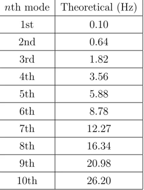
Two simulations, eigenfrequency analysis of a rod with one end clamped and a rod with two ends free, are computed. Eigenfrequencies for these two cas-es are calculated using Equation 2.4 for first ten modcas-es. For rod clamped at one end, theoretical results are computed to compare with simulation results in Table 2.1. Moreover, simulation results of shapes of first three characteristic functions for a vibrating rod clamped at one end are compared with expected results in Figure 2.1. By verifying coherency between theoric and FE simulation for eigenfrequency analysis of a simple object such as a rod, we can also trust on eigenfrequency results of simulations on 3D brain model. In addition, theoreti-cal values of eigenfrequencies computed for a rod free at both ends, are given in Table 2.2.
Figure 2.2: Geometry of the rod used in simulations. nth mode Theoretical (Hz) 1st 0.10 2nd 0.64 3rd 1.82 4th 3.56 5th 5.88 6th 8.78 7th 12.27 8th 16.34 9th 20.98 10th 26.20
Table 2.1: Theoretical values computed by Equation 2.4 for the first 10 eigenfre-quencies of a rod clamped at one end.
nth mode Theoretical (Hz) 1st 0.66 2nd 1.81 3rd 3.56 4th 5.88 5th 8.78 6th 12.27 7th 16.34 8th 20.98 9th 26.21 10th 32.02
Table 2.2: Theoretical values computed by Equation 2.4 for the first 10 eigenfre-quencies of a rod free at both ends.
2.1.2
Cubic Simulation Phantom
Transient shear wave generation and observation is performed, to simulate a basic MRE experiment. Moreover, applying motion to the surface of the phantom is done by prescribing displacement to the surface, which is also how shear waves are generated in MRE experiments. Thus, generating shear waves by prescribing displacement is used in frequency domain analysis of 3D brain model, as will be explained in Section 2.1.3. Therefore, one of the aims of this simulation is learn how to excite head model by generating motion in the desired directions.
Time domain analysis is performed on a cubic phantom having length, depth and width of 8 cm. Same material properties with the rod in Section 2.1.1 are used, except loss modulus is i2 kPa instead of i7kPa, which is the complex part of the shear modulus. These material properties approximately corresponds to a 1.5% agar-agar phantom.
Figure 2.3: Geometry of the cubic phantom used in simulations.
Geometry of the cube used in simulations is given in Figure 2.3. Prescribed displacement, equal to cos(2πf t) (µm), is defined to the green surface in Fig-ure 2.3 in z direction. Simulation is computed for time interval 2.5 to 12.5 ms with time steps of 2.5 ms.
2.1.3
3D Brain Model
A 3D model of brain is developed from segmented brain images [22, 23]. Eigenfre-quency analysis of the brain is performed, using COMSOL Multiphysics (COM-SOL, Sweden) finite element method (FEM) software. The purpose of eigenfre-quency analysis is to search for possible modes of the brain model and understand directions of excitation for the corresponding eigenfrequencies.
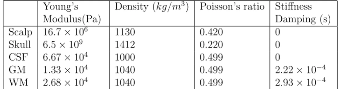
The imported 3D model of the brain is segmented into scalp, skull, cere-brospinal fluid (CSF), gray matter (GM) and white matter (WM). The complete mesh consists 190127 elements. Young’s modulus, Poisson’s ratio and density of the segmented parts are obtained from previous studies [13, 24, 25]. Stiffness damping parameter of Rayleigh damping is used for WM and GM, similar to a previous study [26], and the parameter is set to zero for scalp, skull and CSF. The values of the material parameters used in simulations are given in Table 2.3. In addition, Young’s modulus maps of the brain used in simulations are given in three orthogonal planes Figures 2.4, 2.5, 2.6.
Young’s Modulus(Pa)
Density (kg/m3) Poisson’s ratio Stiffness
Damping (s) Scalp 16.7 × 10⁶ 1130 0.420 0 Skull 6.5 × 10⁹ 1412 0.220 0 CSF 6.67 × 10⁴ 1000 0.499 0 GM 1.33 × 10⁴ 1040 0.499 2.22 × 10⁻⁴ WM 2.68 × 10⁴ 1040 0.499 2.93 × 10⁻⁴
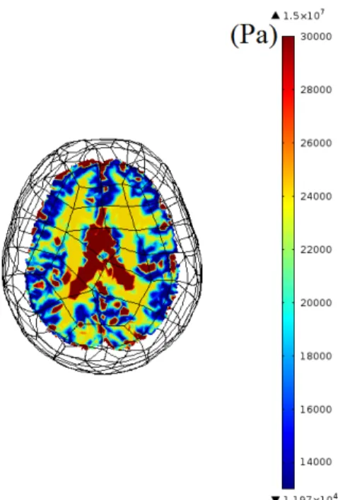
Figure 2.4: Young’s modulus (Pa) map of 3D brain model on transverse plane. Colors for the segmented parts can be translated from the legend as CSF(red), WM(yellow) and GM(blue). Note that skull and scalp are not demonstrated in this map.
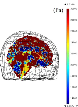
Figure 2.5: Young’s modulus (Pa) map of 3D brain model on sagittal plane. Colors for the segmented parts can be translated from the legend as CSF(red), WM(yellow) and GM(blue). Note that skull and scalp are not demonstrated in this map.
Figure 2.6: Young’s modulus (Pa) map of 3D brain model on coronal plane. Colors for the segmented parts can be translated from the legend as CSF(red), WM(yellow) and GM(blue). Note that skull and scalp are not demonstrated in this map.
In the results of eigenfrequency analysis, modes of rotatory shear waves are observed, which have different eigenfrequencies around different axes of the head and can be excited by conventional actuator systems. Thus, it is decided to carry on with frequency domain analysis simulations, in order to compare eigenfre-quencies with total displacement amplitude response with respect to frequency in frequency domain analysis of exciting these three motions of head.
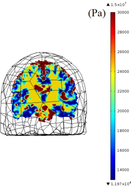
In frequency domain analysis, excitation frequency is swept from 1 Hz to 100 Hz with frequency step of 1 Hz. Peak to peak amplitude of sinusoidal motion induced by pistons to the head at the excitation location is 20 µm. Simulations are repeated for a 10 percent lower Young’s modulus of WM and GM in order to simulate a neurodegenerative disease state [27, 28]. Therefore, for this case Young’s modulus for WM is 24.12 kPa and for GM is 11.97 kPa.
Displacement is measured at the same point on brain model for all simulations. Dependence of shear wave displacement on excitation frequency is analyzed.
2.2
Experiments
MRE Experiments are performed first on phantoms, then on volunteers, to ob-serve shear wave propagation. Experiment results are compared with FE simu-lation results. Observing modes of shear waves in brain MRE simusimu-lations, it is decided to carry on with experiments for investigating possible modes of shear waves in brain MRE experiments.
All experiments are conducted in a 3 Tesla Siemens Tim Trio scanner. Human experiments are performed to analyze possible modes of shear waves on a healthy volunteer, with permission from local board of ethics.
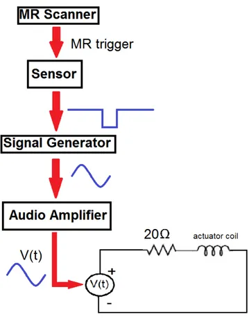
Experimental setup in Figure 2.7 is used for all MRE experiments. Note that for phantom or human experiments with transient excitation, 20Ω resistor is not connected to the coil, as in Figure 2.7. The resistor is only used for human ex-periments with frequency sweeping, in order to eliminate the effect of frequency dependence characteristic of the coil. In other words, we are trying to make a current source out of a voltage source. Hence, a constant peak amplitude for sinusoidal voltage is achieved in frequency range 20-40 Hz. In other experiments, desired voltage amplitude is set by adjusting gain of audio amplifier since fre-quency is not swept.
Figure 2.7: A block diagram for the experimental setup for MRE experiments.
2.2.1
Phantom Experiments
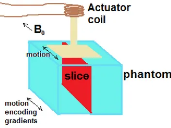
For phantom experiments, 0.8% agar-agar gel is prepared as described in [29]. An actuator coil similar to [30] is implemented. The experimental setup is shown in Figure 2.8. Excitation frequency is 200 Hz. Hence, sinusoidal current at 200
Hz is applied to the coil. Actuator moves in the direction of B0 field sinusoidally,
Figure 2.8: Experimental setup for phantom studies.
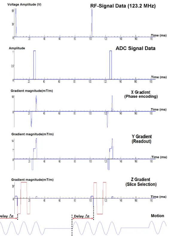
A gradient echo pulse with trapezoidal motion encoding gradient (MEG) is used for acquisition. Frequency of the MEG is set to the same frequency with frequency of excitation, which is 200 Hz. Sequence parameters are T R = 100ms,
T E = 17.5ms, F OV = 300mm, amplitude of MEG GM EG = 30mT /m, number
of MEG NM EG = 2, duration of MEG τM EG = NfM EGM EG = 2002 = 10ms and number
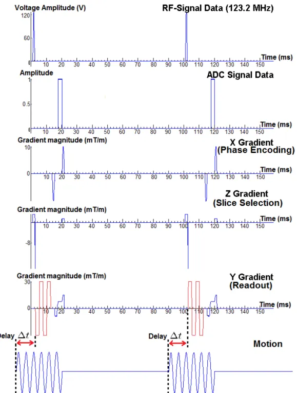
of induced motion cycles in each TR is 6. Two acquisitions are made in each scan by switching polarity of the zeroth moment nulled MEG, having same frequency with excitation frequency, in an interleaved fashion. Pulse sequence is demon-strated in Figure 2.9. Slice orientation is sagittal and direction of MEG is readout direction, which is the direction of the induced motion. 11 images are obtained by changing delay ∆t between beginning of MEG and motion. Motion is induced to actuator before the start of the sequence, according to the amount of delay. Thus, timing of MEG in sequence is constant but timing of motion induced to actuator changes with the delay.
Figure 2.9: GRE sequence with MEG(red waveform) used in excitation frequen-cy sweeping human experiments, with parameters of TR=100ms, TE=17.5ms,
2.2.2
Human Experiments
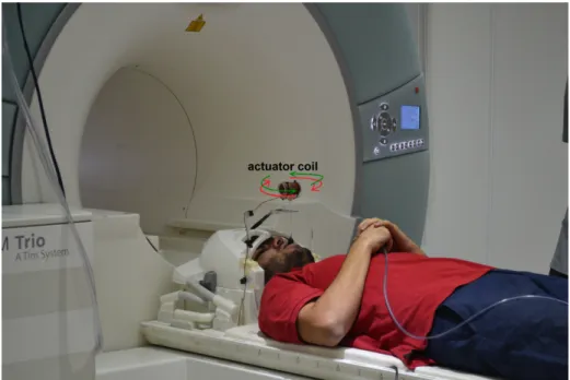
Human experiments are approached in two different analysis: with transient ex-citation and with sweeping exex-citation frequency. In transient exex-citation, conven-tional brain MRE methods are used. Transient analysis is required for the next step, which is frequency response analysis, for setting the experimental method and become able to observe shear waves in brain. Then, we carry our research to a novel investigation, which is mode analysis of shear waves in brain MRE by studying displacement response of shear waves to excitation frequency sweeping. A conventional bite actuator, similar to the implementation in [15] but instead of two coils, only one coil is attached to the actuator, is used for inducing shear waves into brain by forming a similar motion to Indian head bobble. The bite bar is attached to a mouth-guard Thus, volunteer wears the mouth-guard and bite bar transmits motion to the mouth-guard.
A block diagram for the experimental setup is in Figure 2.7. The picture of the volunteer with the bite actuator in MR scanner is in Figure 2.10. When positive voltage is applied to the coil, coil rotates in the direction of one of the arrows in red or green, depending on the cable connections. When negative voltage is applied to the coil, it turns in the opposite rotation direction, in the direction of the other arrow than in case of positive voltage applied. Thus, rotation of the actuator switches between red and green arrows, as sign of the voltage applied switches between positive and negative sinusoidally.
The only difference between sequences of MRE for phantom and brain is shape of MEG. Obtained MRE images for brain with the sequence in Figure 2.9 has motion artifacts, which can be due to breathing or pumping of blood. Therefore, a new pulse shape is generated for MEG by approximately nulling the first moment in addition to the zeroth moment, in order to eliminate motion artifacts caused by motion with constant velocity with respect to MR data acquisition. Pulse shape of zeroth and first moment nulled MEG is shown in Figure 2.11.
Figure 2.10: Picture of experimental setup for brain MRE, demonstrating volun-teer and the bite actuator. Rotation direction of the actuator is shown by red and green arrows. Rotation of the actuator switches between red and green arrows due to the induced sinusoidal current, which provides head bobble motion.
2.2.2.1 Human Experiments with Transient Excitation
Shear waves are induced to the brain at 60 Hz excitation frequency with a bite actuator, as in Figure 2.10. A gradient echo pulse with motion encoding gradient is used for acquisition. 4 cycles of motion are induced and encoded with a single zeroth and first moment nulled MEG. Frequency of the MEG is set to the same
frequency with frequency of excitation, such that fM EG = 60Hz. Other sequence
Figure 2.11: GRE sequence with MEG(red waveform) used in transien-t excitransien-tatransien-tion human experimentransien-ts, witransien-th parametransien-ters of TR=100ms, TE=24ms,
Bite actuator moves the head in head-foot and left-right direction, correspond-ing to head bobble. Note that motion in head-foot direction is more dominant than in left-right direction.
For the first set of images, slice orientation is set to transverse and direction of MEG is set to slice selection, in order to encode motion in head-foot direction, as shown in Figure 2.11. 5 scans are made by incrementing delay between MEG and actuator motion from 37.8 to 54.6 ms with time steps of 4.2 ms.
For the second of images, slice orientation is set to sagittal and direction of MEG is again set to slice selection, in order to encode motion in left-right direction, as shown in Figure 2.11. 5 scans are made for the same delay values with the first set.
2.2.2.2 Human Experiments with Sweeping Excitation Frequency
Experiments are performed to analyze possible modes of shear waves on a healthy volunteer. The motion is induced continuously and frequency of excitation is swept from 20 Hz to 40 Hz, with frequency steps of 2 Hz by a bite actuator as in Figure 2.10.
A gradient echo pulse with motion encoding gradient is used for acquisition. Frequency of the MEG is set to the same frequency with frequency of excitation. Sequence parameters are T R = 250 − 500ms, T E = 32.5 − 57.5ms. The reason of TR and TE parameters’ changing inside an interval is the variability of the duration of the MEG and induced sinusoidal motion due to sweeping frequency.
Slice orientation is set to transverse and direction of MEG is set to slice selection, in order to encode motion in head-foot direction.
An example of the pulse sequence is given in Figure 2.12 and 2.13, for
T R = 60ms, T E = 20ms and having a MEG frequency of 80 Hz. In the first sequence, in Figure 2.12, the phase difference between MEG and actuator motion is 0. In the second sequence, in Figure 2.12, the phase difference is π/2.
Two scans are performed for each frequency, by adjusting the phase of the actuator signal, in order to obtain two phase difference images at steady state of shear waves having π/2 phase difference to each other. In the post-processing part, the root of sum of squares (RSS) of the displacement of these two phase images is obtained. Amount of displacement of shear waves are measured on the same line for all frequencies. In order to eliminate the effect of different amount of induced motion into head caused by frequency dependence of the bite actuator, measured displacements are normalized to displacement of the actuator measured for each excitation frequency by an optical method, explained in [30], while volunteer is biting the actuator in MR scanner.
Figure 2.12: GRE sequence with MEG(red waveform) used in frequency sweep-ing excitation human experiments, with parameters of TR=60ms, TE=20ms,
Figure 2.13: Same sequence with Figure 2.12 except MEG and actuator motion are quadrature phase.
Chapter 3
Results
Similar results for FE simulations and MR experiments of phantom MRE are achieved. Coherency between theoretical computation and eigenfrequency FE simulations of a rod is observed for its characteristics and mode frequencies.
Obtaining shear wave images from brain MRE experiments is accomplished by developed sequence and experimental setup including bite actuator. In eigen-frequency analysis of brain model, modes of shear waves are observed, which can be excited by conventional actuator systems. Frequency domain analysis demon-strates that modes of shear waves can be excited by brain MRE. Experimental results of a preliminary study of modes of shear waves in brain MRE, which is performed on a volunteer are demonstrated.
3.1
Finite Element Simulations
Results for eigenfrequency simulations and computed theoretical natural frequen-cies for a rod are compared. Simulated shear wave images for phantom MRE are presented. Frequency domain analysis for 3D brain model is designed and imple-mented according to eigenfrequency analysis of brain model. Thus, results of two analyses are presented and compared.
3.1.1
A Simple Geometric Object: Rod
Eigenfrequency analysis is performed for the rod in Figure 2.2 with parameters given in Section 2.1.1, for one end clamped case and for two ends free case. Results obtained from simulations and values computed by Equation 2.4 for the first 10 eigenfrequencies of a rod clamped at one end, are compared in Table 3.1. For two ends free case, simulation and theoretical results are compared in Figure 3.2. Percentage errors are computed for comparison, by equation
Percentage Error % = |Simulation − Theoretical|
Theoretical × 100. (3.1)
nth mode Theoretical (Hz) Simulation (Hz) Percentage Error (%)
1st 0.10 0.10 0 2nd 0.64 0.65 1.56 3rd 1.82 1.82 0 4th 3.56 3.55 0.28 5th 5.88 5.81 1.19 6th 8.78 8.59 2.16 7th 12.27 11.85 3.42 8th 16.34 15.56 4.77 9th 20.98 19.68 6.20 10th 26.20 25.04 4.43
Table 3.1: Comparison of results obtained from simulations and values computed by Equation 2.4 for the first 10 eigenfrequencies of a rod clamped at one end.
(a) n=1 at 0.1048 Hz
(b) n=2 at 0.6545 Hz
(c) n=3 at 1.8233 Hz
Figure 3.1: Arbitrary total displacement on a rod vibrating at first three eigen-frequency results, clamped at only one end.
For the rod clamped at one end, the maximum percentage error between eigenfrequencies obtained from simulations and computed by Equation 2.4, is 6.20% for the 9th mode. For the rod free at both ends, the maximum percent-age error between eigenfrequencies obtained from simulations and computed by Equation 2.4, is 6.84% for the 10th mode. These errors are computational er-rors due to the mesh size. As eigenfrequency increases, wavelength of vibration gets smaller. However, wavelength of vibration supported by the mesh size is limited. Hence, computational error increases as eigenfrequency increases. Also, decreasing the size of the meshes, increases size of computation greatly since the simulation object rod is almost a 2D object. Thus, size of computation is chosen as it is supported by the computational limits of the computer.
When simulation results of shapes of first three characteristic functions for a vibrating rod clamped at one end in Figure 3.1, are compared with expected results in Figure 2.1, it is observed that they are coherent with each other.
Validating eigenfrequency results of characteristic functions of a vibrating rod clamped at one end in Figure 3.1 with theoretical characteristic functions in Figure 2.1 and eigenfrequencies computed by simulation with theoretical values in Table 3.1, it is encouraged to proceed with eigenfrequency analysis simulation of a more complex model such as brain.
nth mode Theoretical (Hz) Simulation (Hz) Percentage Error (%)
1st 0.66 0.66 0 2nd 1.81 1.81 0 3rd 3.56 3.53 0.84 4th 5.88 5.79 1.53 5th 8.78 8.56 2.51 6th 12.27 11.81 3.75 7th 16.34 15.52 5.02 8th 20.98 21.44 2.19 9th 26.21 25.73 1.83 10th 32.02 34.21 6.84
Table 3.2: Comparison of results obtained from simulations and values computed by Equation 2.4 for the first 10 eigenfrequencies of a rod free at both ends.
(a) n=1 at 0.6600 Hz
(b) n=2 at 1.8115 Hz
(c) n=3 at 3.5290 Hz
Figure 3.2: Arbitrary total displacement on a rod vibrating at first three eigen-frequency results, free at both ends.
For the rod free at both ends, eigenfrequencies computed by simulation and theoretical values in Table 3.2 are found to be similar with an error less than 6.84%. Eigenfrequency simulation results for characteristic function for the rod free at both ends is given in Figure 3.2.
3.1.2
Cubic Simulation Phantom
For results of cubic phantom, displacement field in z-direction is plotted in central xz-plane and amplitude of the displacement fields is plotted on the central line of the plane in Figure 3.3 and 3.4 for each time step. Propagation of the shear wave can be observed in the results.
(a) t = 2.5 ms
(b) Displacement of (a) on the red line.
(c) t = 5 ms
(d) Displacement of (c) on the red line.
Figure 3.3: Displacement field (mm) in z direction and amplitude of the displace-ment on the central (red) line for each time step. Note that position of the red line is only demonstrated in (a) since it is same for all time points.
(a) t = 7.5 ms
(b) Displacement of (e) on the red line.
(c) t = 10 ms
(d) Displacement of (a) on the red line.
(e) t = 12.5 ms
(f) Displacement of (c) on the red line.
Figure 3.4: Figure 3.3 Cont’d. Displacement field (mm) in z direction and ampli-tude of the displacement on the central (red) line for each time step. Note that position of the red line is only demonstrated in Figure 3.3(a) since it is same for all time points.
3.1.3
3D Brain Model
Results of eigenfrequency analysis demonstrates that brain has modes at certain frequencies for different motions corresponding to nodding, naying, and Indian
head bobble. In Figure 3.5a, 3.5c and 3.5e, total displacement at the first
eigenmodes of Indian head bobble, naying and nodding is demonstrated, respec-tively. Note that computed total displacements are in arbitrary unit, since they are results of eigenfrequency analysis and all the sources are nulled for computa-tion. In Figure 3.5b, 3.5d, 3.5f, corresponding excitation rotation motions, to Figure 3.5a, 3.5c, 3.5e are demonstrated, respectively.
(a) 38.53 + i1.09Hz (b) Indian head bobble
(c) 32.48 + i0.77Hz (d) Naying
(e) 35.88 + i0.88Hz (f) Nodding
Figure 3.5: (a)(c)(e) Total displacement(m) patterns of first eigenmodes of brain and (b)(d)(f) corresponding rotation motions for excitation, respectively.
Eigenfrequency results for Indian head bobble, naying and nodding motion of the head are given in Table 3.3, 3.4, 3.5, respectively. The real parts are the eigen-frequencies and complex parts are related with the loss at that eigenfrequency. As expected, loss increases as the frequency increases.
Eigenfrequency (Hz) 38.53 + i1.09 76.06 + i4.06
Table 3.3: Eigenfrequencies that can be excited by Indian head bobble motion of the head. Eigenfrequency (Hz) 32.48 + i0.77 54.03 + i2.09 58.89 + i2.43 86.17 + i5.24
Table 3.4: Eigenfrequencies that can be excited by naying motion of the head.
Eigenfrequency (Hz) 35.88 + i0.88 79.79 + i4.48
Table 3.5: Eigenfrequencies that can be excited by nodding motion of the head.
In addition to these eigenmodes in Tables 3.3 - 3.5, there are modes of the brain rotating about axes, different than three axes in Figure 3.5. However, geometry of the head is not symmetric about these axes. Therefore, excitation of these modes is difficult and not possible with conventional MRE actuators. Thus, only these three motions are studied in frequency domain analysis.
For the brain model having 10% reduced shear modulus for WM and GM, eigenfrequency results for Indian head bobble, naying and nodding motion of the
head are given in Table 3.6, 3.7, 3.8, respectively. A negative shift is observed in eigenfrequencies obtained for the normal brain model given in Table 3.6, 3.7, 3.8.
Eigenfrequency (Hz) 36.88 + i0.99 76.06 + i4.06
Table 3.6: Eigenfrequencies that can be excited by Indian head bobble motion of the head, for the brain model having 10% reduced shear modulus for WM and GM. Eigenfrequency (Hz) 31.08 + i0.71 51.74 + i1.91 56.50 + i2.22 82.64 + i4.82
Table 3.7: Eigenfrequencies that can be excited by naying motion of the head, for the brain model having 10% reduced shear modulus for WM and GM.
Eigenfrequency (Hz) 34.44 + i0.80 76.03 + i4.18
Table 3.8: Eigenfrequencies that can be excited by nodding motion of the head, for the brain model having 10% reduced shear modulus for WM and GM.
In frequency domain analysis, these modes of brain are excited by inducing rotation to the head by predefining sinusoidal displacement, having 2µm peak to peak displacement, to two pistons with a phase difference of π.
As seen in Figure 3.6 rotation of the head is achieved about the desired axes, since total displacement patterns are similar to the patterns in eigenfrequency analysis results in Figure 3.5.
(a) 39 Hz at phase=0 (b) 39 Hz at phase=π
(c) 32 Hz at phase=0 (d) 32 Hz at phase=π
(e) 36 Hz at phase=0 (f) 36 Hz at phase=π
Figure 3.6: Total displacement(m) at first eigenfrequencies of each rotation mo-tion (a)(b) Indian head bobble, (c)(d) naying, (e)(f)nodding, at phases 0 and π. Note that total displacements in (a,c,e) are in arbitrary units.
Results of frequency domain analysis, by sweeping excitation frequency from 1 Hz to 100 Hz with 1 Hz frequency steps, for three different motions induced by the methods shown in Figure 3.6, are demonstrated by the red curves in Figure 3.7. Frequency domain analysis indicates that displacement of shear waves formed in the brain can increase significantly when brain is excited at its eigenfrequencies with correct excitation at that frequency, since peak displacements match with eigenfrequencies demonstrated by black curves in Figure 3.7. For instance, first mode for Indian head bobble is found at 38.53 + i1.09Hz, where complex part is related to the damping of the mode, and a peak in the displacement is observed in frequency sweeping simulation at 39 Hz.
Note that peak displacements for naying at eigenfrequencies 54.03 + i2.09 and 58.89+i2.43 are combined to form a peak displacement at 57 Hz, as in Figure 3.7b. Repeated frequency sweeping simulations for 10% reduced shear modulus, are demonstrated by the green curves in Figure 3.7. In the case of reduced stiff-ness, frequencies of peak displacements shift but displacement-frequency response function patterns do not change, as seen in Figure 3.7. Similarly, a shift is ob-served in eigenfrequencies for the brain model in neurodegenerative state, given in Table 3.6, 3.7, 3.8.
For the brain model in neurodegenerative state, it is expected to observe a decrease in eigenfrequencies and frequencies of peak displacements in Figure 3.7 since shear modulus of WM and GM are reduced by 10%, by Equation 1.9. In addition, an increase in amplitudes of shifted peak displacements in Figure 3.7, is observed for the brain model in neurodegenerative state. The reason of this raise may be due to the acting damping on each peak displacement is decreased since the corresponding frequencies to the peak displacements decrease for re-duced stiffness simulations. Note that damping decreases as excitation frequency decreases.
For reduced stiffness brain model, a frequency shift is not observed in peak at 76 Hz for Indian head bobble in Figure 3.7a although a shift is observed in eigenfrequency analysis in Table 3.6. Moreover, a decrease in peak displacement is observed at 76 Hz. The reason of this behaviour is open to discussion.
0 10 20 30 40 50 60 70 80 90 100 0 100 200 300 400 500 600 700 Frequency (Hz)
Total Displacement (um)
Normal Brain
10% reduced shear modulus for WM and GM Eigenfrequencies for normal brain
(a) Indian head bobble
0 10 20 30 40 50 60 70 80 90 100 0 10 20 30 40 50 60 70 80 90 100 Frequency (Hz)
Total Displacement (um)
Normal Brain
10% reduced shear modulus for WM and GM Eigenfrequencies for normal brain
(b) Naying 0 10 20 30 40 50 60 70 80 90 100 0 20 40 60 80 100 120 140 160 180 Frequency (Hz)
Total Displacement (um)
Normal Brain
10% reduced shear modulus for WM and GM Eigenfrequencies for normal brain
(c) Nodding
Figure 3.7: Simulation results for displacement versus frequency swept and eigen-frequencies for different motions (a) Indian head bobble, (b) naying, (c) nodding.
Similar shear waves patterns are observed for eigenfrequency and frequency domain analyses. As an example, eigenfrequency results at 38.53 Hz, having an excitation pattern for Indian head bobble, and frequency domain analysis for Indian head bobble at 39 Hz, are compared in Figure 3.8. In Figure 3.8a, 3.8b, displacement fields in orthogonal direction to the slice are demonstrated for eigen-frequency analysis at 38.53 Hz and eigen-frequency domain analysis at 39 Hz. Absolute value of the displacement fields in Figure 3.8a, 3.8b are shown in 3.8c, 3.8d, re-spectively. Absolute value of displacement field on the red line in Figure 3.8c, 3.8d are plotted in 3.8e, 3.8f, in order to emphasize the similarity between two analysis and their similarities to mode patterns.
(a) Eigenfrequency analysis at 38.53+i1.09 Hz.
(b) Frequency domain analysis at 39 Hz.
(c) Absolute value of (a). (d) Absolute value of (b).
(e) Displacement on red line in (c).
(f) Displacement on red line in (d).
Figure 3.8: Displacement fields(m) in orthogonal to slice direction in simulation results (a)eigenfrequency (b)frequency domain. Absolute values of displacements on red line for (a,b) are shown in (d,e), respectively. Note that numerical values in (a,c) are in arbitrary units.
Most importantly, comparison of eigenfrequency and frequency domain anal-ysis emphasizes that modes of shear waves can be observed in brain by exciting head at its eigenfrequencies with correct excitation, as shown in 3.8.
3.2
Experiments
In this section, results of phantom and human MRE experiments are presented. Phantom experiments are performed with transient excitation at 200 Hz induced by the actuator. Human experiments are performed with transient excitation at 60 Hz and frequency sweeping excitation from 20 to 40 Hz, induced by a bite actuator.
3.2.1
Phantom Experiments
Results of the phantom experiments are indicated in Figure 3.9- 3.11. Delay between MEG and motion is changed from 0 ms to 20 ms with time steps of 2 ms. In addition to phase images, phase on a single line, red line shown in Figure 3.9a, is plotted in order to observe the propagation of the shear wave.
−50 −40 −30 −20 −10 0 10 20 30 40 50 (a) ∆t = 0ms 0 50 100 150 200 250 300 −50 −40 −30 −20 −10 0 10 20 Position(pixel) Phase(degrees)
(b) Phase of (a) on the red line.
−50 −40 −30 −20 −10 0 10 20 30 40 50 (c) ∆t = 2ms 0 50 100 150 200 250 300 −60 −50 −40 −30 −20 −10 0 10 20 Position(pixel) Phase(degrees)
(d) Phase of (c) on the red line.
−50 −40 −30 −20 −10 0 10 20 30 40 50 (e) ∆t = 4ms 0 50 100 150 200 250 300 −60 −40 −20 0 20 40 60 Position(pixel) Phase(degrees)
(f) Phase of (e) on the red line.
−50 −40 −30 −20 −10 0 10 20 30 40 50 (g) ∆t = 6ms 0 50 100 150 200 250 300 −60 −40 −20 0 20 40 60 Position(pixel) Phase(degrees)
(h) Phase of (g) on the red line.
Figure 3.9: Phase-difference (degrees) images at each time frame and amplitude of phase-differences on a single line (red line). Note that position of the red line is only demonstrated in (a) since it is same for all time points.
−50 −40 −30 −20 −10 0 10 20 30 40 50 (a) ∆t = 8ms 0 50 100 150 200 250 300 −40 −30 −20 −10 0 10 20 30 40 50 60 Position(pixel) Phase(degrees)
(b) Phase of (a) on the red line.
−50 −40 −30 −20 −10 0 10 20 30 40 50 (c) ∆t = 10ms 0 50 100 150 200 250 300 −40 −30 −20 −10 0 10 20 30 40 50 Position(pixel) Phase(degrees)
(d) Phase of (c) on the red line.
−50 −40 −30 −20 −10 0 10 20 30 40 50 (e) ∆t = 12ms 0 50 100 150 200 250 300 −40 −30 −20 −10 0 10 20 30 40 50 60 Position(pixel) Phase(degrees)
(f) Phase of (e) on the red line.
−50 −40 −30 −20 −10 0 10 20 30 40 50 (g) ∆t = 14ms 0 50 100 150 200 250 300 −50 −40 −30 −20 −10 0 10 20 30 40 50 Position(pixel) Phase(degrees)
(h) Phase of (g) on the red line.
Figure 3.10: Figure 3.9 Cont’d. Phase-difference (degrees) images at each time frame and amplitude of phase-differences on a single line (red line). Note that position of the red line is only demonstrated in Figure 3.9(a) since it is same for all time points.
−50 −40 −30 −20 −10 0 10 20 30 40 50 (a) ∆t = 16ms 0 50 100 150 200 250 300 −50 −40 −30 −20 −10 0 10 20 30 40 50 Position(pixel) Phase(degrees)
(b) Phase of (a) on the red line.
−50 −40 −30 −20 −10 0 10 20 30 40 50 (c) ∆t = 18ms 0 50 100 150 200 250 300 −50 −40 −30 −20 −10 0 10 20 30 40 50 Position(pixel) Phase(degrees)
(d) Phase of (c) on the red line.
−50 −40 −30 −20 −10 0 10 20 30 40 50 (e) ∆t = 20ms 0 50 100 150 200 250 300 −50 −40 −30 −20 −10 0 10 20 30 40 50 Position(pixel) Phase(degrees)
(f) Phase of (e) on the red line.
Figure 3.11: Figure 3.9 Cont’d. Phase-difference (degrees) images at each time frame and amplitude of phase-differences on a single line (red line). Note that position of the red line is only demonstrated in Figure 3.9(a) since it is same for all time points.
3.2.2
Human Experiments
Phase difference images are computed by subtracting two phase images obtained from interleaved sequence having different polarity of MEG.
3.2.2.1 Human Experiments with Transient Excitation
Phase difference images for transverse slice, which demonstrates motion in head-foot direction induced by bite actuator, are in Figure 3.12.
Similarly, phase difference images for sagittal slice, which demonstrates motion in left-right direction induced by bite actuator, are in Figure 3.13.
Shear wave propagation can be observed from images obtained at different time points, both in Figure 3.12 and 3.13. Comparing these figures, displacement in head-foot direction is greater than that of in left-right direction, which is expected since induced motion by bite is more dominant in head-foot direction than in left-right direction.
−60 −40 −20 0 20 40 60 (a) ∆t = 37.8ms −60 −40 −20 0 20 40 60 (b) ∆t = 42ms −60 −40 −20 0 20 40 60 (c) ∆t = 46.2ms −60 −40 −20 0 20 40 60 (d) ∆t = 50.4ms −60 −40 −20 0 20 40 60 (e) ∆t = 54.6ms
Figure 3.12: Phase-difference (degrees) images of human experiment results on transverse plane with transient excitation at 60 Hz and MEG direction of orthog-onal to the slice (head-foot). Acquired images at 5 time points by adjusting the delay(∆t) between MEG and actuator motion.
−60 −40 −20 0 20 40 60 (a) ∆t = 37.8ms −60 −40 −20 0 20 40 60 (b) ∆t = 42ms −60 −40 −20 0 20 40 60 (c) ∆t = 46.2ms −60 −40 −20 0 20 40 60 (d) ∆t = 50.4ms −60 −40 −20 0 20 40 60 (e) ∆t = 54.6ms
Figure 3.13: Phase-difference (degrees) images of human experiment results on sagittal plane with transient excitation at 60 Hz and MEG direction of orthog-onal to the slice (left-right). Acquired images at 5 time points by adjusting the delay(∆t) between MEG and actuator motion.
3.2.2.2 Human Experiments with Sweeping Excitation Frequency
From two transverse phase images, having 0 and π/2 phase difference between MEG in head-foot direction and actuator motion, the root of sum of squares (RSS) of the displacement is obtained. Amount of displacement of shear waves are measured on the same line for all frequencies.
In addition, frequency dependence of amplitude of induced motion by actua-tor is considered. Measured displacements of the bite actuaactua-tor, while volunteer is biting, for each frequency, are used for normalizing the computed RSS displace-ment. By this normalization, it is assumed that induced motion to the brain by the actuator is constant. Frequency dependence of shear wave displacements formed in brain is plotted in Figure 3.14.
20 25 30 35 40 0 0.005 0.01 0.015 0.02 0.025 0.03
Normalized displacement with respect to actuator
Frequency (Hz)
Bite Actuator (Indian head bobble)
Figure 3.14: Displacement of shear waves formed in brain by frequency sweeping excitation between 20-40 Hz, normalized with respect to actuator motion.
In Figure 3.14, peak displacement is observed at 26 Hz. In addition, the human shear wave pattern observed at 26 Hz is similar to the mode at 38.53 Hz of eigenfrequency analysis and 39 Hz of frequency sweeping simulation, as in Figure 3.8 and 3.15. Hence, results of continuous frequency sweeping excitation emphasizes that modes of shear waves can be observed in brain MRE.
−4 −3 −2 −1 0 1 2 3 4 Displacement (um)
(a) Displacement field (µm) in orthogonal direction to the slice, at 26 Hz 0 0.05 0.1 0.15 0.2 0.25 0.3 0 2 4 6 8 Position (m)
Absolute value of displacement in slice selection direction(um)
(b) Absolute value of displacement field on the red line in (a)
Figure 3.15: Human experiment at 26 Hz. (a)Displacement field for the direction orthogonal to slice. (b)Absolute value of displacement on red line.
Chapter 4
Discussion and Conclusion
In this work, a new method to detect changes in stiffness of tissues is proposed, which consists of analyzing modes of shear waves and detecting the frequency shift in peak displacement of shear waves in MRE. To test the accuracy of eigenfrequen-cy analysis in FE simulations, a simple geometric object, whose eigenfrequencies can be computed theoretically is chosen. Eigenfrequencies of a rod are computed by FE simulations. Percentage error between results obtained from simulations and theoretical values computed for the first 10 eigenfrequencies of a rod clamped at one end, is at most 6.20%, as seen from Table 3.1. For the case of a rod free at both ends, the percentage error is at most 6.84%. These errors are computational errors due to the mesh size. In addition, simulation results for total displacement on vibrating rod at its eigenfrequencies and theoretical shapes of characteristic functions for a vibrating rod clamped at only one end, are compared for the first three eigenfrequencies and found to be same, as demonstrated in Figure 2.1 and Figure 3.1. Therefore, eigenfrequency analysis for brain model is proceeded with confidence.
Before proceeding with FE simulations and experiments of MRE of the brain, these analyses are conducted on phantoms. Time domain analysis is performed on a cubic agar phantom model and propagation of shear wave is observed by examining results at different time points. In the simulations, shear waves are induced to the phantom model in a manner similar to inducing shear waves in
MRE experiments, which is prescribing displacement to the surface of phantom. MRE experiments are performed on phantoms and patterns of observed shear waves are in good agreement with simulation images, as in Figures 3.3 and 3.9. Experimental setup is developed for brain MRE. A bite actuator is implement-ed for inducing shear waves into the brain, and modifications on the sequence, used for phantom, are made in order to reduce motion artifacts of the head, for brain MRE. Shear waves in the brain are observed with transient excitation at 60 Hz. As expected, observed displacement in head-foot direction is greater than, that of in left-right direction, due to induced motion by the actuator is also greater in head-foot direction, as seen in Figures 3.12, 3.13.
In the results of eigenfrequency analysis, modes of shear waves are observed for rotation about different axes of head, each having modes at different eigenfre-quencies, given in Figures 3.5. It is realized that these modes can be excited by conventional actuator systems. Furthermore, eigenfrequency results for rotation of head about three different axes, corresponding to naying, nodding and Indian head bobble, are compared to total displacement amplitudes in frequency domain analysis of exciting these three motions of head.
In the results of frequency domain analysis, peak displacements matches with eigenfrequencies as seen in Figure 3.7. For instance, first mode for Indian head bobble is found at 38.53 + i1.09, and a peak in the displacement is observed in frequency sweeping simulation at 39 Hz. In Figure 3.8, similar mode patterns for shear are observed. In the case of reduced stiffness, frequency of peak dis-placements shift but displacement response pattern does not alter, as seen from Figure 3.14. Results of frequency domain analysis indicates that displacement of shear waves formed in brain can increase greatly when brain is excited at its eigenfrequencies with correct excitation direction at that frequency.
The shear displacement measured in brain for MRE experiments is normalized to displacement of actuator, which is measured by an optical method described in [30], for each frequency. Unfortunately, it is not certain that total motion of the actuator is induced to the head. There may be some losses in the transmission of motion. Therefore, developing a method for measuring induced displacement