Automated robotic assembly line design with
unavailability periods and tool changes
Hakan Gultekin*
Department Industrial Engineering,
TOBB University of Economics and Technology, Sogutozu Cad. No. 43, 06560, Ankara, Turkey Fax: +90-312-292-4091
Email: [email protected] *Corresponding author
Adnan Tula
Rotterdam School of Management, Erasmus University,
Rotterdam, The Netherlands Email: [email protected]
M. Selim Akturk
Department of Industrial Engineering, Bilkent University,
06800 Bilkent, Ankara, Turkey Fax: +90-312-266-4054 Email: [email protected]
Abstract: We focus on an assembly line design problem of a fully automated robotic spot-welding line. Different from existing studies, we take the prescheduled unavailability periods, such as lunch and tea breaks, into account in order to reflect a more realistic production environment. This problem includes allocating operations to the stations and satisfying the demand and cycle time within a desired interval for each model to be produced. We also ensure that assignability, precedence, and tool life constraints are met. Furthermore, the existing studies in the literature overlook the limited lives of the tools that are used for production. Tool replacement decisions not only affect the tooling cost, but also the production rate. Therefore, we determine the number of stations and allocate the operations into the stations in such a way that tool change periods coincide with the unavailability periods to eliminate tool change related line stoppages in a mixed model robotic assembly line. We provide a mathematical formulation, propose a two-stage local search algorithm and test the performances of these methods using different problem instances with varying parameters. [Received: 12 November 2012; Revised: 8 February 2016; Accepted: 18 February 2016]
Keywords: robotic assembly line; line balancing; automobile industry; mathematical programming; local search algorithm.
Reference to this paper should be made as follows: Gultekin, H., Tula, A. and Akturk, M.S. (xxxx) ‘Automated robotic assembly line design with unavailability periods and tool changes’, European J. Industrial Engineering, Vol. x, No. x, pp.xxx–xxx.
Biographical notes: Hakan Gultekin is an Associate Professor at the Department of Industrial Engineering at TOBB University of Economics and Technology in Ankara, Turkey. He received his BS, MS and PhD in Industrial Engineering from Bilkent University in Turkey. His research interests include scheduling, optimisation modelling, and exact and heuristic algorithm development, especially for problems arising in modern manufacturing systems, energy systems, and wireless sensor networks.
Adnan Tula graduated in Industrial Engineering from Bilkent University in 2007. He carried out his research on assembly line designs and also received his Masters degree in Industrial Engineering from Bilkent University in 2009. Later, he received his Masters degree in Marketing from CentER Graduate School, Tilburg University in 2010. He is expecting to receive his PhD in Marketing from Rotterdam School of Management, Erasmus University. M. Selim Akturk is a Professor and Chair of the Department of Industrial Engineering at Bilkent University. His recent research interests are advanced manufacturing technologies, production scheduling and airline disruption management.
This paper is a revised and expanded version of a paper entitled ‘Design of a fully automated robotic spot welding line’ presented at International Conference on Informatics in Control, Automation and Robotics (ICINCO ‘11), Noordwijkerhout, The Netherlands, 28–31 July 2011.
1 Introduction
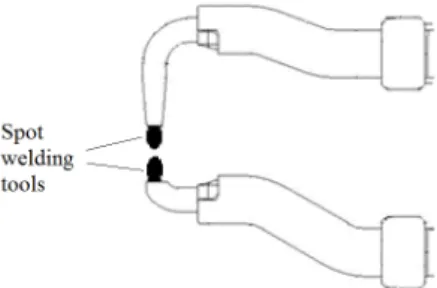
Resistance spot welding is an example of fusion-welding processes that uses a combination of heat and pressure to join sheet-metal parts. It is widely used in mass production of automobiles, appliances, metal furniture, and other products made of sheet metal as discussed in Goover (2007). An important application of robots in the automotive industry is their use for spot welding operations in robotic cells. A robot can repeatedly move the welding gun to each weld location and position it perpendicular to the weld seam. It can also replay programmed welding schedules. Once an automotive component of a vehicle is designed and the required spot welds to assemble the pieces on this component are determined, the problem of allocating the welding operations to robotic cell stations arises. Different allocations result in different production quantities (i.e., cycle times), station investment costs and tooling costs. Each station consists of a single robot in a fully automated production line. In order to perform welding operations, the robots use spot welding guns. Two spot welding tools (also denoted as welding tips or electrode tips) are attached to a spot welding gun as shown in Figure 1. A welding tool has a limited life time, which is represented by the total number of spot welds that it can process. Each robot in the line is assumed to have a different welding tool with a
different lifetime. Spot welding robots should have six or more axes of motion and be capable of approaching points in the work envelope from any angle. This permits the robot to be flexible in positioning a welding gun to weld an assembly. Spot welding robots are generally preferred to manual welding operators because of the weight of the gun and monotony of the task.
Figure 1 A spot welding gun
This study focuses on a robotic cell mixed-model assembly line design problem in which automotive body components are produced. Since multiple product types can be produced in this line in an arbitrarily intermixed sequence, it is called a mixed-model assembly line (Becker and Scholl, 2006). The problem is to determine the number of stations to be established, to allocate the welding operations to these stations with a constraint on the cycle time, and, different from the literature, to determine the tool change periods in order to maximise the total profit.
One may question the validity of integrating an operational issue like the planning of tool change times into the strategic decision of workstation formation and operation allocation. The design problem that we study in this paper is originated from a project that we conducted for one of the leading automotive manufacturing companies in Turkey. One of the important aspects of any design problem is the operational problems that can be faced during the actual implementation of the design. We first investigated the existing automotive body component robotic spot welding assembly line, where the line is fully automated to produce two models in any order. In that project, our aim was to develop a tool change decision policy for the assembly line where there was no systematic approach for scheduling the tool change periods. All of the tools were being changed just at the end of their lives. As a consequence, the line was stopped regularly for tool changes. The company has allocated almost 10% of their available capacity to the line stoppages due to tool changes. Our aim is to eliminate these line stoppages and hence increase the throughput rate. This is the main reason why we study line design and operation allocation problems together with the scheduling of tool change periods.
Today, improvements in technology and automation and large investment costs incurred for building assembly lines have increased the importance of studies on designing efficient assembly lines. Therefore, numerous studies have been conducted by researchers, in which different aspects of assembly line design problems are considered such as the layout of the line, equipment selection and line balancing. As stated in a survey paper by Boysen et al. (2007), there are two main groups of assembly line studies. Simple assembly line balancing (SALB) problems consider a single product to be produced in the line. For a review of studies in the SALB field, we refer to the review paper by Scholl and Becker (2006). The second group is called the general assembly line balancing (GALB) problems, in which SALB problems are extended by
introducing other aspects such as mixed-model or multi-model cases, zoning constraints and parallel stations. As described by Becker and Scholl (2006), in a mixed-model line, different models are produced in an arbitrary inter-mixed sequence. Several studies consider mixed-model lines. Erel and Gokcen (1999) used a shortest-route formulation to solve a mixed-model ALB problem. Common assembly tasks between different models are assigned to the same station. Scholl et al. (2010) studied an assembly line balancing problem with assignment restrictions. Guschinskaya and Dolgui (2009) studied a transfer line balancing problem. Kahan et al. (2009) studied operational issues of a robotic assembly line in an automotive industry. They proposed a mixed-integer linear programming based recovery plan to rebalance the line during repair, when one of the robots has failed to perform its assigned tasks. Wilhelm and Gadidov (2004) devised a branch-and-cut approach to minimise the total assembly system cost that includes station activating, machining and tooling costs considering machine capacities and available tool spaces in the stations. On the other hand, Andres et al. (2008) and Scholl et al. (2013) studied assembly line balancing and scheduling problem with sequence dependent setup times due to walking distances or tool changes. Traditional assembly line design studies are generally based on the objectives of minimising the cycle time, number of stations or total costs; or maximising the efficiency of the assembly lines.
In this study, different from the studies in the literature, we address a mixed-model assembly line problem with a profit maximising objective. We aim to determine the number of stations to open, which affects the station installation costs and the throughput rate; the assignment of operations to the stations, which affects throughput rate and tool usage (as a consequence the tooling cost); and tool change periods, which affect cycle time and tooling costs. Therefore, the relevant terms for the total profit function are the individual profits from each manufactured component (revenue minus all the costs except the tooling and station installation costs), tooling cost, and station installation cost. As a consequence, we define the total profit function as the difference between the sum of individual profits gained by manufacturing components of the final products and the sum of investment costs for stations and tooling. Station investment costs include robot, fixture and space costs. Tooling costs are incurred over time as the tools are changed with new ones.
Prior studies do not consider the unavailability periods of assembly lines and assume that assembly lines work 24 hours a day continuously. However, in practice, lines stop several times a day for lunch and tea breaks. In this study, we take such breaks into account to reflect a more realistic production environment. We deal with designing a mixed-model assembly line that works 24 hours a day in three 8-hour shifts and each shift includes a lunch break and two tea breaks in which the line stops operating. Since the preceding manual stations feeding the required components to the robotic line stop during these breaks, the fully automated robotic spot-welding line has to stop as well.
A few prior studies have addressed tool selection and costs. However, these studies ignore the fact that tool lives are limited and incorporate the assumption that tooling costs are incurred only once at the beginning. In Gultekin et al. (2006, 2010), we dealt with the robotic cell scheduling problem with two identical CNC machines and a single material handling robot. We already showed that the previous theoretical results on the same problem were no longer valid when we added the tool life related constraints to the problem setting since the cycle times depend on the allocation of the operations.
The tool life has a number of implications in the current problem setting as well: Continuing to use a tool even after its life is over results in quality problems and, thus, tools must be changed. On the other hand, replacing a tool before its life is over increases the tooling cost. Additionally, the life of a tool may end at a time instant when the assembly line is supposed to be operating and therefore may result in line stoppages which, in turn, reduces the production rate. As already mentioned, tool lives are represented by the total number of spot welds that they can perform before wearing out. We propose the lunch and tea breaks in which the line is not operating as tool change periods by which we aim to eliminate tool change related line stoppages. At each break, if there exist welding tools that have a remaining number of spot welds less than the total number of spot welds that they have to perform until the next break, they must be changed with new ones. With such an operating rule and by assigning the operations to the stations considering not only the cycle times but also the tool usage rates at each station, we prove that the total profit can be increased.
We could state the contributions of this paper as follows. First, to the best of our knowledge, this paper is an initial attempt at developing a comprehensive mathematical model for a fully automated robotic spot-welding line. Although most of the current literature addresses manual assembly lines, there are few studies on automated assembly lines as summarised in Boysen et al. (2008). They also state that there is a clear need for new approaches and algorithms to solve real-world balancing problems for fully automated lines, such as spot welding robots in our case, that can capture both the flexibility of these systems as well as their limitations. Second, through tool availability constraints, we explicitly formulate limited tool lives of spot welding guns allowing us to incorporate line stoppages due to tool changes in the initial design level. We also take into account unavailability periods, and assign tasks to robotic stations in a way that tool replacement periods coincide with unavailability periods. Our study is the first one that considers unavailability periods and tool changes due to the limited tool lives while designing a fully automated robotic spot-welding line. Moreover, the number of required spot welds for each operation may not be the same, and hence the operation allocation decisions without considering their impact on the tool replacement decisions might necessitate unnecessary line stoppages.
The remainder of the paper is organised as follows: in the next section we present a nonlinear mixed-integer programming (NLMIP) formulation of our assembly line design problem. The linearised mixed integer version of this formulation is provided in the Appendix. In Section 3, we propose a two-stage local search algorithm for finding good feasible solutions in a reasonable computational time. We show the computational effectiveness of the proposed algorithm by comparing with an exact method in Section 4. Section 5 is devoted to the concluding remarks.
2 Problem definition
In this section, we give a formal definition of the problem and introduce the parameters, variables and the mathematical programming formulation we use to solve our problem. We consider an assembly line that contains at most m stations: S1, S2, . . . , Sm. Let
M = {1, 2, ..., m} be the set of indices of these stations. Space restrictions in the
production area and a limited budget for investment costs are among the reasons of such a restriction on the number of stations. We use parameter Vjto denote the cost of setting
up station j, j∈ M. At the same time, the proposed formulation could be viewed as a reconfiguration planning of an existing system with a given number of stations, since the fully automated assembly line could already be set up and operating, and changing the number of stations (or adding additional stations) on the line may not be possible. Using the proposed formulation, we could find a new allocation of the operations to different stations, whenever there is a substantial model mix change, while guaranteeing that the tool life, precedence and availability constraints are satisfied.
There are g different models (product types) to be produced in this robotic assembly line and G = {1, 2,..., g} is the index set of these models. Ohi represents operation
i of model h, i∈ Nh, h∈ G, where Nh = {1, 2, ..., nh} is the index set of welding operations to be allocated to stations for model h and nh is the number of operations to be performed to produce model h. A number of spot welds is grouped together to form an operation. The selection is based on the closeness of the welds to each other and to
satisfy the proper geometry of the assembled components. Let Whi be the number of
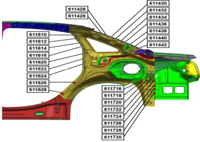
spot welds required to perform operation i on model h, i∈ Nh, h∈ G. The total number of spot welds that the welding tool in station j∈ M can process before its life is over is denoted by Bj. An example of an automotive body component is given in Figure 2. This figure shows the spot welds required to perform some of the welding operations on different locations of the part. The 26 spot welds seen in this figure constitute a subset of all welds required to produce this body component.
Figure 2 A spot weld scheme of an automotive body component (see online version for colours)
Factors that affect the number of stations to be opened are the target cycle time, the station investment cost, and the tooling cost. Let us represent the yearly expected demand for the parts to be produced as θh, h∈ G. We use the parameter γh to denote the target cycle time for model h to meet the yearly expected demand, θh. This target cycle time includes any allowances for equipment failures and other similar downtimes. This is a procedure that is used in literature for assembly lines with stochastic task times (Becker and Scholl, 2006) and such a procedure increases the stability of the
solutions where the parameters are considered to be deterministic (Sotskov et al., 2006). Considering stochastic machine failures complicates the problem a lot but still worth studying.
In general, let Th be the total time allocated for production of model h in annual terms; fh the actual cycle time of model h; and bθh the corresponding production quantity. Then, we have the following:
bθh=
Th
fh
∀h. (1)
Once the actual cycle times are determined for the produced models, then their actual production levels can also be determined. The mixed model production is carried out in Minimal Part Set (MPS) mode, i.e., the smallest possible set of parts in the same proportion as the actual annual production levels is determined and this set is repetitively processed in a cyclic mode.
Producing model h less than a specified quantity is not acceptable. The cycle time corresponding to this production quantity will specify an upper bound on the cycle time. Let this value be denoted by γU
h and the corresponding production quantity be
denoted by θU
h. Additionally, if production exceeds a certain quantity for each model, it is not possible to make any additional profit. The cycle time corresponding to this production quantity will specify a lower bound on the cycle time. Let this value be denoted by γL
h and the corresponding production quantity be denoted by θLh. Clearly, we have θU
h ≤ θh≤ θhL. Note that, the reference for the lower (L) and upper (U) bounds is the cycle time. Additionally, the individual profit gained from model h is assumed to be a piecewise linear function. If the actual production amount of model h is less than the annual demand (bθh≤ θh), the profit is denoted by P Rh. On the other hand, if the actual production amount of model h exceeds the annual demand (θh< bθh≤ θhL), then the profit for each model h produced as surplus is denoted by P Rϵ
h, such that
P Rϵh= P Rh− ∆h, 0≤ ∆h≤ P Rh, (2)
where ∆h denotes the reduction in the individual profit for the excess parts when the production exceeds the expected demand. As a consequence, the individual profits from each model h is a two-piece linear function where the slope of the second piece is less than that of first piece. It is important to note that this term does not include the station investment cost and the tooling cost. As a consequence, the individual profit of model
h is calculated as follows: bθh· P Rh if γh≤ fh≤ γhU, (3) θh· P Rh+ (bθh− θh)· P Rϵh if γ L h ≤ fh< γh, (4) θh· P Rh+ (θLh − θh)· P Rϵh if fh< γhL. (5) We consider tool change times as decision variables. If tools are only changed at scheduled breaks as we propose, the line will never stop for a tool change, which increases the throughput rate; but on the other hand, some tools will be changed before their lifetimes are over. Therefore, the tooling cost will be increased. As a result, one aim of this study is to determine the impact of increased tooling cost on throughput rate.
In most of the automotive companies (including the one with which we have been collaborating), plants work 24 hours in three 8-hour shifts and there are several breaks in an 8-hour shift. In general, there is a 10-minute break at the beginning of a shift for shift change, a 10-minute tea break, a 30-minute lunch break and a second 10-minute tea break in each shift, e.g., corresponding to 1 hour 45 minutes (6,300 seconds) between each break. In this study, we propose using these breaks as tool change time periods. In any break, if the remaining life of a welding tool is less than the total number of welds it has to perform until the next break, it needs to be changed during that particular break. As a result, tooling cost may increase since the tool is changed before its lifetime is over; but, on the other hand, a line stoppage is prevented, which has more severe implications. Let Cjbe the cost of tools assigned to station j, j ∈ M and U be the total number of breaks in the planning horizon. We also need the following decision variable:
zjq = 1, if tools in station j∈ M are changed in tool change period q,
q = 1, 2, . . . , U ;
and 0, otherwise.
Using these, the required tool change time is the following:
K + µ·
m ∑ j=1
zjq ∀q = 1, 2, . . . , U, (6)
where K is a constant denoting the time to prepare for the tool change and µ is another constant that corresponds to the time required to change the two welding tools on a single welding gun.
In order to decide on the tool change times, one must be able to calculate the remaining life of each tool at each break for which the consumption of each tool between two breaks must be known. However, these consumptions depend on the state of the stations as well as the part sequence in a mixed model assembly line. Furthermore, because of the deviations between the cycle time values of different models and the deviations between the processing times of different stations on the line, there may be starvation and blocking situations. These complicate the calculation of tool consumptions and thus the remaining tool lives. Because of these complexities, we will approximate the remaining tool lives as discussed below, and the validity of these approximations is tested with a simulation study later on.
For this approximation, we define the parameter ψh for h = 1, . . . , g as the ratio of the total yearly required time to process all demanded parts of model h to total yearly required time to process all demanded parts of all models. This ratio is the time allocated for production of parts of model h and can be calculated as follows:
ψh=
θh· γh ∑g
l=1θl· γl
∀h ∈ G. (7)
Let ξ denote the production time between two breaks. In our computational study it is used as 6,300 seconds. In order to approximate the remaining tool life at each break we calculate the time allocated for the production of parts of all models between two breaks as ξ· ψh seconds and use these values in our mathematical model.
As it is seen in Figure 2, a large number of spot welds is required to complete the production of a component. Depending on the location of these welds and the geometry
of the component, it may not be possible for a particular type of welding gun to reach every location and the special characteristics of the weld such as the diameter and the thickness may require a different welding tool. Therefore, it is not possible to process all spot welds by one type of welding gun and corresponding welding tool. Thus, we define the following parameter indicating feasible assignments:
ahij = 1, if operation i∈ Nh of model h∈ G can be assigned to station j ∈ M; and 0, otherwise.
The assembly of some components may prevent the reach of the welding gun to some of the welding operations. Hence, these operations must be performed before this component is assembled. For such cases, we define a precedence matrix P and use the following parameter:
phik = 1, if operation i∈ Nh of model h∈ G precedes operation k ∈ Nh
of model h∈ G;
and 0, otherwise.
From industrial practice, it is evident that although different robots and tools are able to perform some spot welds, the difference in their processing times for the same operation is negligible. Therefore, we assume the processing time of an operation to be independent of the station at which it is processed. Let thi be the time required to perform operation i∈ Nhof model h∈ G. We calculate thias a function of the number of spot welds required to perform operation i of model h as follows:
thi= α + β· Whi ∀h ∈ G, i ∈ Nh, (8)
where α is a constant that denotes the time required for the robot to reach to the location to perform operation i of model h and β is another constant that corresponds to the time required to process a single spot weld.
In summary, the individual profit gained from producing model h is assumed to be a piecewise linear function of production quantity as defined in equations (3) to (5) and hence we need model-specific cycle times, fh, in order to calculate the production quantity of model h. Furthermore, tool lives are represented by the total number of spot welds, and the number of required spot welds for each operation i of model h, Whi, may not be the same. Therefore, we have to keep track of the production quantities of each model, i.e., equivalently individual cycle times for each model, fh, to approximate the remaining tool lives (and corresponding tool replacement periods at each station,
zjq).
In addition to decision variables fh and zjq, we will use the following decision variables to formulate our problem:
Rjq remaining number of spot welds that the welding tool in station j
can process after tool change period q, j = 1, 2, . . . , m, q = 1, 2, . . . , U
σj = 1, if station j∈ M is used in the assembly line; and 0, otherwise
xhij = 1, if operation i∈ Nh of model h∈ G is assigned to station j ∈ M; and 0, otherwise.
Having defined the parameters and the decision variables of our problem, the nonlinear mixed-integer mathematical program can be formulated as follows:
Formulation 1 (NLMIP): Max g ∑ h=1 P Rh· min { θh· γh fh , θh } + g ∑ h=1 P Rϵh· min { max { θh· γh fh − θh, 0 } ,θh· γh γL h − θh } (9) − ρ · m ∑ j=1 U ∑ q=1 Cj· zjq− η · m ∑ j=1 Vj· σj Subject to fh≥ τj+ nh ∑ i=1 thi· xhij ∀h, j (10) fh≤ γhU ∀h (11) xhij ≤ ahij· σj ∀h, i, j (12) m ∑ j=1 xhij = 1 ∀h, i (13) phik· j ∑ l=1 xhil+ (1− phik)≥ xhkj ∀h, i, j, k (14) Rjq= Bj· zjq + [ Rj(q−1)− g ∑ h=1 ξ· ψh fh · nh ∑ i=1 Whi· xhij ] (1− zjq) ∀j, q (15) Rj0= Bj ∀j (16) Rjq≥ g ∑ h=1 ξ· ψh fh · (nh ∑ i=1 Whi· xhij ) ∀j, q (17) fh≥ 0, Rjq≥ 0, xhij, σj, zjq∈ {0, 1} ∀h, i, j, q (18) The objective function is a piecewise linear function that includes the individual profits that can be earned by producing up to θh parts of model h and the reduced profits for the situation of producing more than θh as well as the tooling and station investment costs. The tooling cost term that appears in our objective function is a function of the total number of tools used throughout the planning horizon. Tooling and station costs are converted to annual costs by the constants ρ and η, which depend on the selection of the total number of tool change periods in the planning horizon, U , and the number of months that the production of the selected models will continue, respectively. Constraint (10) ensures that the cycle time is the maximum station time, which is the sum of the operation times allocated to that station plus a constant τj required for the robot in station j to begin and finalise processing the allocated operations. Constraint
(11) prevents the actual cycle time for model h from exceeding γU
restricts operations to be assigned only to the stations where they can be performed and to stations which are used in the assembly line. By (13), we ensure that an operation is assigned to exactly one station and none of the operations remains unassigned. Constraint (14) allows an operation to be assigned to a station if all its predecessor operations are assigned to the same or to a preceding station. Constraint (15) is a coupling constraint that connects different models to compete for a limited tool life at each station. It also handles updates for the remaining number of spot welds for welding tools. If the tool is changed at that tool change period, the life time of the tool is reset. Otherwise, the remaining tool life is calculated by subtracting the number of spot welds performed during the last working period from the tool life at the beginning of this working period. As already mentioned this calculation is an approximation that assumes the production amount of each model in each working period is proportional to its actual annual production level. We assume that in the beginning of the planning horizon new tools are loaded. These are initialised in constraint (16). By constraint (17), we guarantee that none of the welding tools finishes its lifetime between two breaks.
In this study, it is assumed that there are enough workers to handle the required number of tool changes in a particular tool change period. However, in some cases, there may be a restricted workforce for tool changes. Let Dq be the available time in tool change period q, q = 1, 2, . . . , U . Then, the following constraint, which ensures that we do not spend more than available time in a particular tool change period, can be inserted to Formulation 1: K + µ· m ∑ j=1 zjq ≤ Dq ∀q = 1, 2, . . . , U. (19)
Furthermore, there might be pairs of welds that cannot be performed at the same station because of the incompatibility between these tasks. In order to handle such restrictions, we could introduce a new 0-1 parameter rhik to our mathematical formulation. If the operations i and k of model h are incompatible, then this parameter takes the value of 1. Then, we should include the following set of constraints to Formulation 1:
xhil+ xhkl≤ 2 − rhik, ∀h, i, k, l (20)
so that these operations can be prevented for being assigned to the same station. In this section, we have defined our problem, the parameters and the decision variables; and formulated the problem as an NLMIP. We could also state that our problem is NP-hard in the strong sense since it can be reduced to 3-partition problem (Lenstra et al., 1977). In order to solve this NLMIP formulation, we could use DICOPT, a nonlinear solver included in GAMS software. The computational study on this formulation is presented in Section 4. However, since the initial tests on realistic datasets showed that the NLMIP is not efficient in terms of computation time, we reformulated the problem as a MIP by linearising the objective function as well as the constraints. The linearised formulation (Formulation 2) can be found in the Appendix. As we will see further in Section 4, even finding a feasible solution by solving MIP using CPLEX with a time limit of two hours may not be possible for several instances. Therefore, we propose a computationally more efficient algorithm below.
3 Proposed two-stage algorithm
In this section, we will present the proposed two-stage algorithm. In the first stage, our aim is to determine a set of initial feasible solutions for the overall problem, which will be called as Algorithm 1. The second stage, denoted as Algorithm 2, corresponds to an improvement phase in a local search algorithm. In this framework, Algorithm 1 generates a feasible solution in each iteration. A feasible solution will be denoted by the vector of decision variables of Formulation 1 as y = (fh, Rjq, xhij, σj, zjq). Since each iteration starts with a different cycle time upper bound (i.e., γU
h), it results in a distinct feasible solution that are stored in set S. Therefore, Algorithm 1 performs a search for different initial feasible solutions corresponding to different cycle time values over the intervals [γL
h, γhU] for h∈ G. In order to improve these initial solutions in Algorithm 2, we reformulate the above NLMIP as a mixed integer problem so that this new formulation can efficiently be solved by any commercial LP solver. By obtaining a set of feasible solutions rather than a single solution at the end of Algorithm 1, we increase our chance of escaping from local optima in the second stage of the algorithm. The proposed two-stage algorithm outputs the required number of stations and an optimal allocation of each spot welding operation that satisfy the assignability, cycle time, precedence, and finally tool life constraints. Furthermore, it also schedules the tool change periods and determines at which break each of the welding tools in the assembly line should be changed.
3.1 Stage 1: finding initial feasible solutions
We start the first stage by using the original upper bounds of the cycle times for each model h∈ G (bγU
h = γ U
h in the initialisation step of Algorithm 1). We solve for a feasible cycle time (fh) value for each model. In the next iteration, we reduce the upper bound of the cycle time for each model (bγU
h = fh− ∆t) and recalculate feasible cycle time values. We continue in this manner as long as bγU
h ≥ γLh for each h∈ G as outlined in Algorithm 1. We used ∆t = 1 in our experiments.
Each iteration of the algorithm generates a feasible solution. In an iteration we first create a list I of unassigned operations, which initially includes all operations and becomes empty (I = Ø) when all of the operations are allocated to the stations. Then, by using precedence matrix P , we create a list, pred(h, i), that includes all predecessor operations of operation Ohi, ∀i, h. Instead of using this original list, we generate a copy of this list, dpred(h, i), and update this copy during the run in order not to lose information from one major iteration to the next. An operation is assignable when its predecessor list, dpred(h, i) is empty. In order to satisfy the cycle time and tool life constraints, we keep the information about total time spent and total number of spots performed for a particular model in each station using loadhj and spothj, respectively. Initially, loadhj = τj and spothj = 0,∀h, j.
After these initialisations, we start allocating the spot welding operations to stations. The operations are allocated one at a time. Therefore, a total of ∑gh=1nh steps is required in each iteration for allocating all operations. Operations are allocated in a sequence of decreasing operation times and they are allocated to the stations starting with the minimum indexed one. This procedure resembles the longest processing time (LPT) rule which is one of the most popular techniques used in bin packing
and scheduling problems (Pinedo, 2012) and used widely in assembly line balancing literature. Four important constraints are considered during this allocation:
1 assignability constraint
2 cycle time constraint
3 precedence constraint
4 tool life constraint.
Once an operation is allocated to a station, it is removed from I. loadhj and spothj are updated for the station that the operation is allocated, and the operation is removed from the predecessor lists dpred(h, i) of those other operations for which the allocated operation is a predecessor. After all operations are allocated, objective function value for the corresponding solution is calculated using equation (9). Let φy denote this value. In order to generate another feasible solution, the upper bound on the cycle time for model h∈ G, bγU
h, is changed and the allocation procedure is repeated.
3.2 Stage 2: improvement algorithm
Since Algorithm 1 allocates one operation at a time in each iteration, it may not necessarily lead to an optimal allocation of operations. For a feasible solution y∈ S found at the end of Algorithm 1, let my be the corresponding number of stations and (fh)y be the corresponding cycle time value for each model h∈ G. Achieving lower cycle times than these (as long as they are feasible) without increasing the number of stations increases the revenue term in equation (9). Therefore, in this subsection, we first reformulate our MIP formulation, denoted as Formulation 2 in the Appendix, to minimise the maximum cycle time for a given my value attained from Algorithm 1 for each feasible solution y∈ S. Since the new formulation will be solved for each feasible solution found in Stage 1, we would like to retain the feasibility and to reduce the computational requirements as much as possible without sacrificing from the optimality to certain extent as depicted in Algorithm 2.
In the improvement algorithm, we solve the following reduced problem without decision variables zjq, denoted as Formulation 3, for each feasible solution.
Formulation 3 (reformulation for each feasible solution y):
Minimise MaxCycleTime + g ∑ h=1 ((fh)y− γhL) (21) Subject to MaxCycleTime≥ (fh)y ∀h (22) m ∑ j=1 σj≤ my (23)
Constraints (2.1) to (2.5), (3.1), (4) to (6) of Formulation 2 in the Appendix
Bj≥ g ∑ h=1 ξ· ψh· (nh ∑ i=1 Whi· ehij ) ∀j (24) (fh)y, ωh≥ 0 ∀h, xhij, σj∈ {0, 1} ∀h, i, j (25)
Algorithm 1 Heuristic for finding initial feasible solutions
*+,-&m∈ 345 g ∈ 345 nh +,&h= 1, . . . , g5 65 75 Whi +,&h= 1, . . . , g5 i = 1, . . . , nh5
) Bj 0-.τj +,&j= 1, . . . , m5 γh5γUh 0-. θh +,&h= 1, . . . , g8 . /-&,-&S5 0 ($) ,+ +$0('21$ (,1%)',-9(: 0 12"%+ 3 %+%&%4!%52 6 bγU h = γhU ∀h ∈ G 7 S= ; 8 9'%!2∃bγU h ,!+2 "2%"bγUh ≥ γhL :# ; <&$0)$ 1'()I )=0) *,-)0'-( 011 ,>$&0)',-( Ohi5h= 1, . . . , g5 i = 1, . . . , nh <
<&$0)$ >&$.$*$((,& 1'() >&$.(h, i) +,& $0*= Ohi5h∈ G5 i ∈ Nh +&,?P
)=
%+%&%4!%52 ))
d
>&$.(h, i) = >&$.(h, i)5 loadhj= τj, spothj= 0 +,& 011 h = 1, . . . , g5
).
i= 1, . . . , nh, j= 1, . . . , m
)0
9'%!2I6= ; :#
)3
@'-. 0- ,>$&0)',-Ohi∈ I A')= d>&$.(h, i) = ; 0-. ?0B'?%? thi
)6 6(('/- Ohi), ()0)',-Sj A')= ?'-'?%? >,(('21$ '-.$B (%*= )=0) )7 ahij C D )8 loadhiEthi ≤bγUh );
phik·Pjl=1xhil+ (1 − phik) ≥ xhkj +,& $0*=k∈ >&$.(h, i)
)<
ξ·ψh
?0B{?0Bk∈M \j{loadhk},loadhj+thi}· (spothj+ Whi) +
.= X ¯ h∈G\h ξ·ψ¯h ?0Bk∈M{load¯hk}· spot ¯ hj≤ Bj loadhj= loadhj+ thi .) spothj= spothj+ Whi .. I= I \ {Ohi} .0 d
>&$.(c, d) = d>&$.(c, d) \ {Ohi} +,& 011 Ocd∈ I
.3 F$)y 2$ )=$ *,&&$(>,-.'-/ (,1%)',-.6 <01*%10)$ϕy5 )=$ *,&&$(>,-.'-/ ,2G$*)'H$ +%-*)',- H01%$ .7 S= S ∪ y .8 fh← ?0Bj∈M{loadhj} ∀h ∈ G .; bγU h ← fh− ∆t ∀h ∈ G (%*= )=0) fh> γhL .< 2+: 0=
Algorithm 2 Algorithm for improving heuristic solutions
*+,-&m∈ 456 g ∈ 456 nh,&'h = 1, . . . , g6 #6 76 Whi,&'h = 1, . . . , g6 . i = 1, . . . , nh6 Bj 8/9τj ,&'j = 1, . . . , m6 γh6γUh 8/9θh ,&'h = 1, . . . , g: ) /-&,-&" ;02) 2&$1)(&/ 01"%+ 2 <1/ #$%&'()*+ = 3 4#$ &*+, -$./0(%,1 2 3/$#%(/)y∈ S 5# 6
>&$.0 ?&'+1$8)(&/ @ A()* )*0 28+0 -8'8+0)0'2 8/9 ,(/9 ¯y 7 BC 38$31$8)(/% 3&''02-&/9(/%zjq 8/9Rjq .8$102 8 ¯ S = ¯S∪ ¯y 9 ?(/9mmin : 4#$mˆy= mmin%/ 1()y∈S{my} − 1 5# .;
>&$.0 ?&'+1$8)(&/ @ A()*my= myˆ8/9 ,(/9 ˆy6 .. BC 38$31$8)(/% 3&''02-&/9(/%zjq 8/9Rjq .8$102 .) ˆ S = ˆS∪ ˆy .2 D8$31$8)0ϕy6ϕ¯y 8/9ϕˆy 12(/% 0E18)(&/ F=GH ,&' 083*y∈ S6 ¯y∈ ¯S 8/9 .3 ˆ y∈ ˆS
Best← 8'%+8Iy∈S,¯y∈ ¯S,ˆy∈ ˆS{+8I{+8Iy∈Sϕy, +8Iy∈ ¯¯ Sϕy¯, +8Iy∈ ˆˆ Sϕyˆ}} .6
1+5
.7
In this new surrogate objective function, we minimise the maximum cycle time to
increase the revenue for a given value of my. However, in order to maximise the
revenue, besides the maximum cycle time the individual cycle times of each model must also be minimised. This is the reason behind the second term of the objective function in Formulation 3. The new non-negative decision variable, ehij= xhij· wh, which is used in Formulation 2 in the Appendix, appears in Formulation 3 as well. In this formulation, we find an optimal allocation for each feasible solution y due to the objective function [equation (21)] and constraint (22). The right hand side values of these constraints are passed from Algorithm 1. Furthermore, the constraint sets of (15), (16) and (17) in the NLMIP formulation (i.e., Formulation 1) are replaced with a new constraint set (24) since zjq variables are not used in this new formulation. It is important to note that we can easily derive the values of Rjqand zjq afterwards to attain a solution (¯y) for Formulation 1. Constraint (24) guarantees that ¯y is still a feasible
solution for Formulation 1. We run Formulation 3 for a given my stations to minimise the cycle times. However, the new solution may not necessarily improve the objective function value, given in equation (9), due to tooling costs since we have removed the zjq variables in Formulation 3 to ease the computational requirements. In order to enlarge our solution space and generate a set of new feasible solutions, we determine mmin, the minimum number of stations required to find a feasible solution to our original problem. Consequently, we also run Formulation 3 for [mmin, . . . , (miny∈S{my} − 1)] stations with the original problem parameters, calculate Rjq and zjq values, and obtain
the corresponding feasible set of solutions denoted by ˆy. We calculate their objective
function value denoted by φyˆ. We compare φy, φy¯, and φyˆ with each other and report
the best one.
4 Application examples
In this section we provide two examples originated from real life data for the application of the developed two-stage algorithm.
Example 1: An automotive company is planning to set up a robotic assembly line to
produce parts for two different models of cars (g = 2). Next year, the company plans to sell 150,000 cars of the first model (θ1= 150, 000) and 75,000 cars of the second
model (θ2= 75, 000). To achieve this production amount, the company sets a target
cycle time of 76 seconds for both models (γh= 76 for h = 1, 2). In order to meet the orders received so far, a cycle time of at most 80 seconds should be satisfied for both models (γU
h = 80 for h = 1, 2). Market research shows that the company can not sell cars more than the amount that can be produced when the cycle time is 60 seconds for both models (γL
h = 60 for h = 1, 2). Cost analysis shows that up to the production amount of 150,000 for the first model and 75,000 for the second model, each part produced will contribute a profit of $10 (P Rh= 10 for h = 1, 2). In case of producing more than the expected demand, each excess parts produced will contribute an expected profit of $7 for both models (P Rϵ
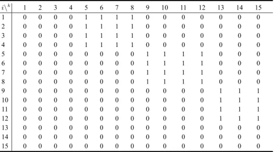
h= 7 for h = 1, 2). In the production area, there is available space for at most ten stations (m = 10). The cost of setting up one station in the assembly line is $192,500 (Vj= 192, 500 for j = 1, 2, . . . , 10). The welding tools have a tool life of 3,200 spot welds (Bj= 3, 200 for j = 1, 2, . . . , 10) and each welding tool costs $10 (Cj = 10 for j = 1, 2, . . . , 10). Both models require 15 spot welding operations (nh= 15 for h = 1, 2) and the number of spot welds required to perform these operations are 10, 8, 8, 7, 10, 9, 8, 7, 10, 9, 7, 6, 13, 12 and 10, respectively. The time required for a robot in a station to reach to the position to perform an operation, the time required to perform a single spot weld and the time required for a robot to begin and finalise processing the allocated operations are calculated to be 1, 2 and 3 seconds, respectively (α = 1, β = 2, τj = 3 for j = 1, 2, . . . , 10). An operation can be allocated to any station (ahij = 1 for h = 1, 2, i = 1, 2, . . . , nh, j = 1, 2, . . . , 10) and the precedence relations between the welding operations for both models are given in Table 1.
When we solve Example 1 using Algorithm 1, we generate seven feasible solutions shown as points in Figure 3. This figure depicts the cycle times of the seven feasible solutions and their corresponding values for the components of the objective function one at a time, as well as the total profit. As seen in this figure, total revenue, which is the sum of the individual profits that each product contributes, strictly decreases as the cycle times increase. Station cost is a non-increasing function with respect to the cycle times because lower cycle times require higher number of stations and it exhibits a stepping structure due to the breakpoints that correspond to particular cycle times.
Table 1 Precedence matrix for Example 1 i\k 1 2 3 4 5 6 7 8 9 10 11 12 13 14 15 1 0 0 0 0 1 1 1 1 0 0 0 0 0 0 0 2 0 0 0 0 1 1 1 1 0 0 0 0 0 0 0 3 0 0 0 0 1 1 1 1 0 0 0 0 0 0 0 4 0 0 0 0 1 1 1 1 0 0 0 0 0 0 0 5 0 0 0 0 0 0 0 0 1 1 1 1 0 0 0 6 0 0 0 0 0 0 0 0 1 1 1 1 0 0 0 7 0 0 0 0 0 0 0 0 1 1 1 1 0 0 0 8 0 0 0 0 0 0 0 0 1 1 1 1 0 0 0 9 0 0 0 0 0 0 0 0 0 0 0 0 1 1 1 10 0 0 0 0 0 0 0 0 0 0 0 0 1 1 1 11 0 0 0 0 0 0 0 0 0 0 0 0 1 1 1 12 0 0 0 0 0 0 0 0 0 0 0 0 1 1 1 13 0 0 0 0 0 0 0 0 0 0 0 0 0 0 0 14 0 0 0 0 0 0 0 0 0 0 0 0 0 0 0 15 0 0 0 0 0 0 0 0 0 0 0 0 0 0 0
Figure 3 Cost and profit values for Example 1 (see online version for colours)
21 22 23 24 25 26 27 55 60 65 70 75 80 R e v e n u e (x 1 0 5)
Cycle Time (sec)
Revenue 6 7 8 9 10 11 12 55 60 65 70 75 80 S ta ti o n C o st (x 1 0 5)
Cycle Time (sec)
Station Cost 1,2 1,3 1,4 1,5 1,6 1,7 1,8 55 60 65 70 75 80 To o li n g C o st (x 1 0 5)
Cycle Time (sec)
Tooling Cost 11,5 12 12,5 13 13,5 14 55 60 65 70 75 80 To ta l P ro fi t (x 1 0 5)
Cycle Time (sec)
Total Profit
This example provides an insight about our problem and the nonlinearity of our objective function. As mentioned previously, the NLMIP formulation and a linearised version of this formulation may not be solved in reasonable computation times using commercial solvers.
In Example 1, the largest objective function value corresponds to the solution in which the actual cycle time is equal to target cycle time, fh= γh, for both models. Since all objective function terms depend on the values of cycle times, this may not always be the case as shown in the next numerical example, and a slight change in problem parameters might lead to a new optimal solution.
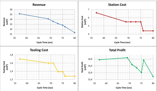
Example 2: Let us reconsider the data of Example 4. However, suppose that γL h = 65 for h = 1, 2 instead of 60 and the cost of setting up one station is decreased to $110,000 (Vj= 110, 000 for j = 1, 2, . . . , 10) instead of $192,500. All the other data remain the same. For this example, Figure 4 shows the values for the individual objective function terms and the objective function value as a whole (total profit) for the corresponding cycle times.
Different total profit value patterns depicted in Figures 3 and 4 show that our problem is difficult in the sense that total profit is a ‘very nonlinear function’ according to the DICOPT solutions manual. Furthermore, Figure 4 clearly shows that the total profit function is neither convex nor concave, and it has multiple local optima. Even for the instances of NLMIP that can be solved by DICOPT, the provided solution may be a local optimum (since DICOPT has no guarantee of providing global optimum). An example for the application of the second stage (Algorithm 2) is provided within the context of computational study in the next section.
Figure 4 Cost and profit values for Example 2 (see online version for colours)
21 22 23 24 25 26 55 60 65 70 75 80 R e v e n u e (x 1 0 5)
Cycle Time (sec)
Revenue 4 5 6 7 55 60 65 70 75 80 S ta ti o n C o st (x 1 0 5)
Cycle Time (sec)
Station Cost 1,2 1,4 1,6 1,8 55 60 65 70 75 80 To o li n g C o st (x 1 0 5)
Cycle Time (sec)
Tooling Cost 15,4 15,9 16,4 16,9 55 60 65 70 75 80 To ta l P ro fi t (x 1 0 5)
Cycle Time (sec)
Total Profit
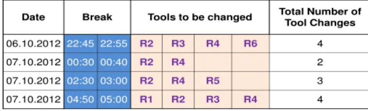
As mentioned previously, the design problem that we study in this paper is originated from a project that we conducted for one of the leading automotive manufacturing companies in Turkey. One of the important aspects of any design problem is the operational problems that can be faced during the actual implementation of the design. The company uses the welding management system (WMS), version 2.94, which is a software developed for welding operations by Gf Welding S.p.A. company, to control the fully automated line. The required information about the current time and the remaining number of spot welds that each tool can perform is stored here. After scheduling the tool change periods, in order to send these to the production area, we prepared an interface for the workers. A snapshot of this interface can be seen in Figure 5 in which a shift-based summary of tool changes is depicted. Based on the current data obtained at any time, we can easily report the necessary tool changes for
each break of the current shift due to constraint (24) in Formulation 3. The workers can check these from a monitor in the production area. This provides the workers an aid for tracing and performing tool changes.
Figure 5 A monitoring of shift-based tool changes (see online version for colours) Date Break Tools to be changed Total Number of
Tool Changes 06.10.2012 22:45 22:55 R2 R3 R4 R6 4 07.10.2012 00:30 00:40 R2 R4 2 07.10.2012 02:30 03:00 R2 R4 R5 3 07.10.2012 04:50 05:00 R1 R2 R3 R4 4 5 Computational study
In this section, we will evaluate the performances of the proposed algorithm and the mathematical formulations solved by GAMS solvers. Algorithm 1 and Algorithm 2 are coded in C++ environment, GAMS-DICOPT2X-c is used as the NLMIP solver and CPLEX version 10.1 is used as the MIP solver. The tests are made on a machine with Pentium Dualcore 1.73 GHz CPU and 1,024 MB of RAM.
The data used in this part of the study is selected as it is faced in the industrial practice. There are two important factors that affect the size of our problem and optimal allocations in the solutions. The first one is the number of different models that will be produced in the robotic cell assembly line, denoted as g. As this parameter increases, our problem becomes harder to be solved by the commercial solvers DICOPT or CPLEX. The second one is the ratio of the profit contribution of the models to the station investment cost, denoted as P RhV
j . This ratio is very important to evaluate the tradeoff between the revenue and the number of stations. We set two levels as low and high for both of these factors. For the number of models, g = 2 is used for the low and g = 4 is used for the high levels. The cost of setting up one station is a constant and selected as Vj = 180, 000 for j = 1, 2, . . . , m. When the ratio P RVjh is at its low level, P Rhis a uniform random number from the interval [5,7]. When this ratio is at its high level, this interval is changed to [9,11]. Using all combinations of these two factors and taking five replications from each combination results in a total of 20 different randomly generated runs.
The value of the parameter nh, the number of spot welding operations required
for model h, is a uniform random number from the interval [8,15]. The value of the parameter Whi, the number of spot welds required to perform operation i of model h, is also a uniform random number from the interval [6,15]. In all the runs, we used
m = 10 for the upper bound on the number of stations that can be used in the assembly
line. We used a constant value of three seconds for the parameter τj, j = 1, . . . , m and a constant value of $10 for Cj, j = 1, . . . , m for the cost of welding tools. The values of the parameters Bj, j = 1, . . . , m are uniform random numbers from the interval [3,200, 4,000]. These values are selected considering the values of the tool lives in the real life project that we have conducted before. We fix the operational parameters as
When the number of models is at the low level, we use θ1= 150, 000 and θ2= 75, 000 and at the high level, we use θ1= 100, 000, θ2= 50, 000, θ3= 50, 000
and θ4= 25, 000 for the values of expected demands. We set the value of the expected
profit for each excess production of model h as P Rϵh=⌈P Rh· 0.7⌉.
In order to set the values of the cycle time lower bound (γhL), cycle time upper bound (γhU) and target cycle time (γh) parameters for a particular model h, we use the following procedure. First, we calculate ¯thi, the average time to perform one spot welding operation of model h. We then round 3· ¯thi to the nearest integer and use this value for γL
h. For γ U
h, 4· ¯thi is rounded to the nearest integer and used. The value of the parameter γh is a uniform random number from the interval [3.3· γhL, 3.6· γ
U h]. Since it is the most difficult and challenging case, in all these runs, we assumed that a welding operation can be assigned to any station (ahij = 1 for h = 1, . . . , g,
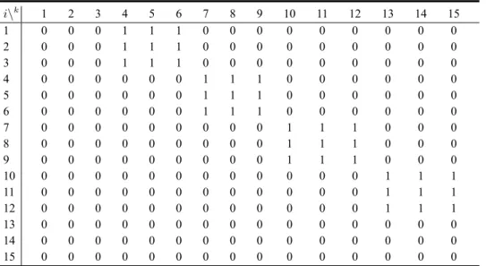
i = 1, 2, . . . , nh, j = 1, 2, . . . , m). Finally, we use the (nhxnh) upper left submatrix of the precedence matrix depicted in Table 2 for the welding operations of model h.
Table 2 Precedence matrix for computational study runs
i\k 1 2 3 4 5 6 7 8 9 10 11 12 13 14 15 1 0 0 0 1 1 1 0 0 0 0 0 0 0 0 0 2 0 0 0 1 1 1 0 0 0 0 0 0 0 0 0 3 0 0 0 1 1 1 0 0 0 0 0 0 0 0 0 4 0 0 0 0 0 0 1 1 1 0 0 0 0 0 0 5 0 0 0 0 0 0 1 1 1 0 0 0 0 0 0 6 0 0 0 0 0 0 1 1 1 0 0 0 0 0 0 7 0 0 0 0 0 0 0 0 0 1 1 1 0 0 0 8 0 0 0 0 0 0 0 0 0 1 1 1 0 0 0 9 0 0 0 0 0 0 0 0 0 1 1 1 0 0 0 10 0 0 0 0 0 0 0 0 0 0 0 0 1 1 1 11 0 0 0 0 0 0 0 0 0 0 0 0 1 1 1 12 0 0 0 0 0 0 0 0 0 0 0 0 1 1 1 13 0 0 0 0 0 0 0 0 0 0 0 0 0 0 0 14 0 0 0 0 0 0 0 0 0 0 0 0 0 0 0 15 0 0 0 0 0 0 0 0 0 0 0 0 0 0 0
Having defined the dataset that we use in our runs, we now continue with some numerical results of our computational study. First, we solve each run with Algorithm 1 and Algorithm 2. Then, we run DICOPT to solve Formulation 1 and CPLEX to solve Formulation 2 for a maximum time limit of two hours (i.e., 7,200 seconds) in order to find solutions for NLMIP and MIP versions of our instances, respectively. We provide these solutions for our original problems under the names DICOPT 1 and MIP 1. In order to improve DICOPT and CPLEX performances, we provide the best Algorithm 1 solutions as initial solutions to these formulations and run them with these initial solutions. We call these solutions as DICOPT 2 and MIP 2.
Table 3 compares the solutions provided by Algorithm 1 and Algorithm 2 in terms of total profit values. The percentage increase in the total profit values is calculated as follows:
IAlg2−Alg1=
(Algorithm 2 value)− (Algorithm 1 value)
In order to obtain the solutions provided in Table 3, we first use Algorithm 1 to attain a set of initial feasible solutions. For each of these solutions, we determine the cycle times, the total profit value and the number of stations required. Afterwards, we implement the improvement algorithm (Algorithm 2). The best solutions attained at the end of Algorithms 1 and 2 are listed in Table 3. Table 4 provides more details about the steps of the algorithms considering run #1 as an example, in which two models are being assembled. The cycle time values of these two models are provided side by side in this table. These results clearly indicate that the optimum cycle time values for different models may not necessarily be the same. The best total profit value found by Algorithm 1 is 460,055. In this solution, the revenue gained as the sum of the individual profits of the parts produced is 1,522,055, a total station cost of 900,000 for setting up five stations and a total tooling cost of 162,000 are incurred. We should also emphasise that we could find a better objective function value for a given number of stations and cycle time upper bounds through better allocation of operations at the end of Algorithm 2. For example, for the same problem instance an optimal solution of Formulation 3 is 507,430, which corresponds to IAlg2−Alg1 = (507, 430− 396, 069)/396, 069 = 28.1% improvement. The number of stations might also be different for these solutions, such that the best Algorithm 1 solution requires five stations, which is 4 in Algorithm 2. In this optimal allocation, the revenue is 1,357,030 but the total station cost and the total tooling cost decrease to 720,000 and 129,600, respectively. Although less revenue is gained, a larger total profit value is achieved as a result of the decrease in the cost terms. Moreover, in spite of solving several MIP formulations at the second stage of the proposed algorithm, the CPU times, expressed in terms of seconds, are quite low compared to the other exact approaches.
Table 3 Total profit values for Algorithm 1 and Algorithm 2
Factor
Replication Run # Algorithm 1 Algorithm 2 IAlg2−Alg1 Algorithm 2
h P R
Vj CPU time (sec)
L L 1 1 460,055 507,430 10.3 3.5 2 2 460,200 557,526 21.2 2.7 3 3 699,150 699,150 0.0 5.6 4 4 354,909 399,544 12.6 3 5 5 583,862 622,650 6.6 3.8 L H 1 6 1,443,553 1,493,919 3.5 2.8 2 7 1,232,202 1,339,032 8.7 2.7 3 8 1,351,146 1,509,570 11.7 2.3 4 9 1,321,299 1,321,299 0.0 4 5 10 1,882,792 1,882,792 0.0 2.2 H L 1 11 668,407 713,824 6.8 8.4 2 12 478,329 583,417 22.0 13.4 3 13 401,048 453,502 13.1 262.6 4 14 586,373 634,184 8.2 7.1 5 15 657,755 723,984 10.1 14.6 H H 1 16 1,516,720 1,558,088 2.7 4.2 2 17 1,663,509 1,725,291 3.7 8.4 3 18 1,200,298 1,272,524 6.0 32.9 4 19 1,042,092 1,130,496 8.5 363.3 5 20 1,205,923 1,210,876 0.4 214.6
Table 4 Calculation of total profit values for Algorithm 1 and Algorithm 2 for run #1
Cycle time Algorithm 1 Algorithm 1 Number Achievable Algorithm 2 Algorithm 2 upper cycle total profit of stations with my− 1 cycle total profit
bounds times values (my) stations? times values
88–88 87–86 396,069 4 No 76–83 507,430 86–85 81–83 453,340 4 No 76–83 507,430 80–82 76–74 378,247 5 No 60–68 479,839 75–73 74–70 411,340 5 No 60–68 479,839 73–69 68–68 460,055 5 No 60–68 479,839 67–67 64–60 308,939 6 No 60–55 308,939
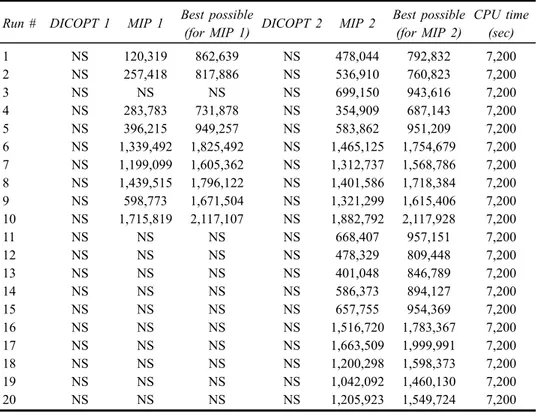
Table 5 Total profit values for DICOPT 1, MIP 1, DICOPT 2 and MIP 2
Run # DICOPT 1 MIP 1 Best possible DICOPT 2 MIP 2 Best possible CPU time
(for MIP 1) (for MIP 2) (sec)
1 NS 120,319 862,639 NS 478,044 792,832 7,200 2 NS 257,418 817,886 NS 536,910 760,823 7,200 3 NS NS NS NS 699,150 943,616 7,200 4 NS 283,783 731,878 NS 354,909 687,143 7,200 5 NS 396,215 949,257 NS 583,862 951,209 7,200 6 NS 1,339,492 1,825,492 NS 1,465,125 1,754,679 7,200 7 NS 1,199,099 1,605,362 NS 1,312,737 1,568,786 7,200 8 NS 1,439,515 1,796,122 NS 1,401,586 1,718,384 7,200 9 NS 598,773 1,671,504 NS 1,321,299 1,615,406 7,200 10 NS 1,715,819 2,117,107 NS 1,882,792 2,117,928 7,200 11 NS NS NS NS 668,407 957,151 7,200 12 NS NS NS NS 478,329 809,448 7,200 13 NS NS NS NS 401,048 846,789 7,200 14 NS NS NS NS 586,373 894,127 7,200 15 NS NS NS NS 657,755 954,369 7,200 16 NS NS NS NS 1,516,720 1,783,367 7,200 17 NS NS NS NS 1,663,509 1,999,991 7,200 18 NS NS NS NS 1,200,298 1,598,373 7,200 19 NS NS NS NS 1,042,092 1,460,130 7,200 20 NS NS NS NS 1,205,923 1,549,724 7,200
The results for DICOPT 1, MIP 1, DICOPT 2 and MIP 2 instances are given in Table 5. The best possible values given in this table are the total profit values of the most promising nodes in the Branch-and-Bound trees of the corresponding runs when the runs are stopped after two hours. The results shown in Table 5 give us insights about the complexity of our problem as well. NS stands for ‘no solution’. DICOPT 2 and MIP 2 solutions are obtained by starting the runs using the Algorithm 1 solutions as initial solutions. By this way, the solution quality is increased in 95% of the problems solved by CPLEX (all except run # 8). Furthermore, the gaps between the best possible and the best solution found after 2 hours is decreased by 42.2% on the average. However, still none of the solution values found by MIP 2 is better than Algorithm 2 solutions.
Up until now, we were able to show that in all of the instances, we can find better solutions with Algorithm 2 than the ones that can be found by solving Formulation 2 using CPLEX with or without initial solutions. Although very few, there may be instances in which MIP 1 can find a solution that is better than the one that can be found by MIP 2 in terms of total profit value. Therefore, while comparing Algorithm 2 and Formulation 2, we take the best of MIP 1 and MIP 2 solutions for the corresponding runs. The percentage of the difference in total profit Values between the best of MIP 1 and MIP 2 and Algorithm i (Alg(i), i = 1, 2) solutions is calculated by the following formula in which F2 represents Formulation 2:
DAlg(i)−F 2
=(Algorithm i value)− (Best of MIP 1 and MIP 2 value)
(Best of MIP 1 and MIP 2 value) × 100. (27)
As we mentioned before, we run DICOPT and CPLEX with a time limit of 2 hours (7,200 seconds) for each of the DICOPT 1, MIP 1, DICOPT 2 and MIP 2 versions of our 20 runs. As it can be seen in Table 5 all formulations hit the time limit in all of the 20 runs. Considering all 20 runs, by Algorithm 2, we are able to find solutions that are on the average 6.0% better than the corresponding best of MIP 1 and MIP 2 solutions in terms of the total profit value. Furthermore, Algorithm 2 performs much better in terms of CPU times with respect to solving Formulation 1 or Formulation 2 using DICOPT or CPLEX, respectively. CPU times for Algorithm 2 can be seen in Table 3. The CPU time of this algorithm increases if a solution found by Algorithm 1 requires a relatively large number of stations (i.e., runs 13, 19, and 20). This is because, as the number of stations increases, the search space of the algorithm also increases. However, Algorithm 2 is very efficient in terms of CPU time requirements even for these cases in comparison to DICOPT and CPLEX formulations.
In order to further test the developed formulations, we selected two instances (runs 1 and 6 listed in Table 3 (first replications of the first two instance clusters)) and ran CPLEX using their MIP 2 formulations without time limits, on a computer with 8 GB memory, Xeon 2.66 GHz CPU and Linux operating system. These instances are selected since the number of models is 2 and they are relatively easier to be solved by CPLEX. However, after 72,660 seconds (20 hours and 11 minutes) and 45,840 seconds (12 hours and 44 minutes) for the runs 1 and 6, respectively, CPLEX terminated due to ‘out of memory’ error since the tree sizes grew to 4.5 GB. The best integer solution found for run 1 was 507,430, which is also the total profit value that we found by Algorithm 2. At this point CPLEX reported an optimality gap of 5.7% with an upper bound of 536,671. The best solution found for run 6 had a total profit value of 1,509,221, which is only 1% better than the total profit value that we found by Algorithm 2. The optimality gap for this case is reported to be 2.5% with an upper bound of 1,546,606. These results imply that Algorithm 2 is capable of finding very good solutions to a very difficult design problem.
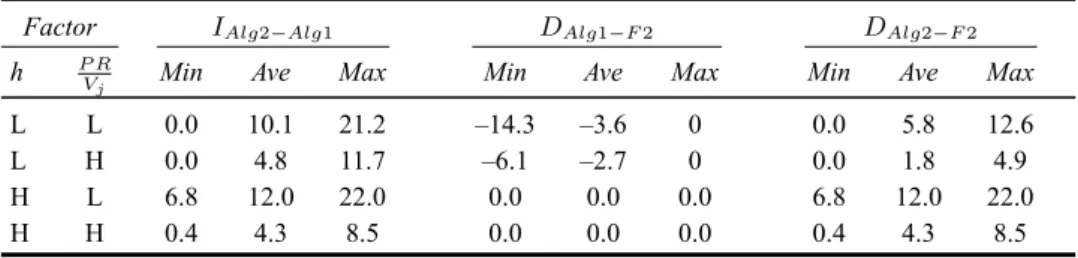
Overall results are sensitive to the selected experimental factors, i.e., the number of different models to be produced in the assembly line and the ratio P Rh
Vj . Table 6 is a summary of the comparative analysis of Algorithm 1, Algorithm 2 and an exact approach of solving Formulation 2 for each factor combination. When h is high, in all of the runs we obtain better results with Algorithm 2 than Algorithm 1. This is because, as the number of models increase, it is more probable to improve the Algorithm 1
allocations at the second stage of the proposed algorithm. The improvements are more significant especially in the runs with low P RhV
j ratios because the total profit values are relatively smaller when P RhV
j ratios are at the low level and as a result, improvements on Algorithm 1 solutions in terms of total profit values correspond to higher percentages. Additionally, Algorithm 1 never finds better solutions than the best of Formulation 1 and Formulation 2, whereas, Algorithm 2 never results in worse solutions than these formulations.
Table 6 Solution analysis for problem clusters
Factor IAlg2−Alg1 DAlg1−F 2 DAlg2−F 2
h P R
Vj Min Ave Max Min Ave Max Min Ave Max
L L 0.0 10.1 21.2 –14.3 –3.6 0 0.0 5.8 12.6
L H 0.0 4.8 11.7 –6.1 –2.7 0 0.0 1.8 4.9
H L 6.8 12.0 22.0 0.0 0.0 0.0 6.8 12.0 22.0
H H 0.4 4.3 8.5 0.0 0.0 0.0 0.4 4.3 8.5
In the proposed mathematical programming formulations, we have used an
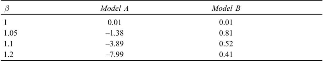
approximation of the remaining tool lives to calculate the tooling cost and tool replacement decisions. In order to test the impact of this assumption on our computational results we have conducted a simulation study to validate our results. The main factors that may affect these approximations are the part mix in the MPS, the difference of the cycle times of different models, the states of the stations at the beginning of each working period (which may be different from each other), and the difference of processing times of the stations from each other. We simulated an automated assembly line with four stations producing two different models (A and B) and tried different combinations for all these factors. In the considered line, there are no buffers between the stations. Therefore, a part cannot be unloaded from a station unless the following station is empty (blocking) and after a station is unloaded, it cannot be reloaded unless the operation in the previous station is completed (starvation). Because of these, the number of parts produced (which is proportional to the number of spot welds performed) by each station in each working period is mainly determined by the bottleneck station. One working period of ξ = 6, 300 seconds is simulated for each parameter combination and in order to analyse the effect of station states on the approximation, the simulation is replicated for 20 times without initialising the system. The number of parts produced by each station from each model in each working period is used as the basis of comparison.
All results are summarised in Table 7. In order to test the effect of difference of model cycle times to approximation, we set model A cycle time to 59.5 seconds
and model B cycle time to 59.5× β seconds and used four different values for β as
can be seen in this table. Theoretical (approximated) values for the number of parts produced in one working period are calculated by allocating the available working time to models with respect to their ratios in the MPS. For example, when A:B ratio is 1:3, 6, 300×1
4 = 1, 575 seconds are allocated to Model A and 6,300–1,575 = 4,725
seconds are allocated to Model B. If β = 1.1 then 1,575/59.5 = 26.47 parts of Model
A and 4, 725/(1.1× 59.5) = 72.19 parts of Model B are found. When theoretical and