ness in MENA Countries
Siibidey Togan
Over the last decade, policymakers, business groups, and economists have argued that improving international competitiveness should be a major policy goal. After considering the meaning of the concept of ‘competitiveness’ in Section 1, in Section 2 the chapter studies issues related to the determination of competitiveness indicators. While Section 3 discusses empirical determina-tion of real effective exchange rates indices, Secdetermina-tion 4 considers other indices of competitiveness based on trade data. Section 5 studies the relation between export performance and real effective exchange rates. The chapter concludes with a summary of results.
1. Competitiveness
One definition of competitiveness is the ability of firms located in the country to sell their output in foreign markets and to compete in domestic markets with output produced in foreign countries. In this case, competitiveness is measured in terms of relative prices and costs with respect to main competitors on the one hand and with respect to main suppliers of imported commodities on the other. The major statistical indicators used are the deflators of GDP and of total exports, producers’ prices, unit labor costs, and market shares. The “Economic Outlook” published by the OECD Secretariat reports three different measures of relative competitiveness. These measures are based on the ratio between domestic and competitors’ average values of manufactured exports, unit labor costs in manufacturing, and consumer price indices expressed in a common currency. The OECD also produces indices of nominal effective exchange rates. A similar approach is also taken by the EU. The calculations of compet-itiveness indicators and nominal effective exchange rates of the OECD and EU use the methodology reported in Durand et al. (1992) and Turner and Van’t dack (1993).
Dollar and Wolff (1993) define a competitive country as one that can suc-ceed in international trade via high technology and productivity, with accom-panying high income and wages. They assert that the best overall measure of competitiveness is productivity. According to the authors, labor productivity indicates the extent to which a country can be a competitive, low-cost ducer while maintaining high wages. On the other hand, the total factor
pro-Bilkent 'Universtty
Siibidey Togcm
ductivity (TFP) measures the output produced by given amounts of labor and capital together, and a high TFP means that both capital and labor can earn large returns while the cost of production remains low. A nation with high labor productivity and high TF P is one that can compete internationally with high incomes and a high standard of living. Hatsopoulos, Krugman, and Summers (1988) take a similar viewpoint. They point out that productivity growth is the fundamental problem. After emphasizing the close relation between capital formation and economic growth they assert that the invest-ment/GDP ratio in the US has been lower than the investinvest-ment/GDP ratio in Japan mainly as the cost of capital in the US has been higher than the cost of capital in Japan.
Forstner (1995) emphasizes that in a world where relative endowments with resources differ among countries and where these factors are not com-pletely mobile across national boundaries, factor abundance is one of several sources of international competitiveness. He asserts that policies which increase competition in a given country also reinforce the impact of compara-tive advantage forces on the country’s international competicompara-tiveness. According to Forstner, a crucial factor for competitive advantage in manufac-turing is physical capital, and semi-skilled labor is the major determinant of comparative advantage at the industry level. A similar approach has been taken by Hughes (1993). He considers trade performance of low, medium and high technology industries in the European Union, the US and Japan and asserts that the main determinants of European trade performance relative to the US and Japan measured by indices of revealed comparative advantage (RCA) are competition, technology and innovation, human capital and physical capital.
The concept of competitiveness used in the White Papers of the United Kingdom and European Commission involves aspects different from those considered above. According to the White Paper ofthe European Commission (1994), competitiveness is the ability ofthe country to reconcile growth with full employment of resources under external equilibrium. The UK White Paper on competitiveness prepared by the Department of Trade and Industry (1995) defines the term as the degree to which the country can, under free and fair market conditions, produce goods and services which meet the test of interna-tional markets, while simultaneously maintaining and expanding the real incomes of its people over the long run. The elements used in these reports to define competitiveness are quite close and they are also similar to those used by the Competitiveness Policy Council in the US and UNICE (1997) in Europe. In brief, competitiveness in these reports can be described as follows: A country is competitive if concurrently its productivity increases at a rate which is similar to or higher than that of its major partners with a comparable level of development, it maintains external equilibrium in the context of an open free-market economy, and it realizes a high level of employment.
The White Paper of the European Commission (1994) contains a wide range of proposals aiming at increasing competitiveness through (i) full exploitation of internal market, (ii) trans-European networks, (iii) technologi-cal research and development, (iv) promotion of new technologies, (v) open-ing towards rest of the world, (vi) improvements in human capital via educa-tion and retraining, and (vii) other elements promoting the productivity of the community economies. On the other hand the UK White Paper on competi-tiveness published by Department of Trade and Industry (1998) identifies ten areas that influence competitiveness: 1. macroeconomy, 2. education and train-ing, 3. labor market, 4. innovation, 5. management, 6. fair and open markets,
7. finance for business, 8. communications and infrastructure, 9. commercial
framework, and 10. Business of the government and public procurement. Most of the proposals aimed at increasing competitiveness in the EU and UK White Papers on Competitiveness are found in the new theories of endo-geneous growth summarized by Barro and Sala-i-Martin (1995). In the neo-classical model of economic growth of Solow (1957) the production function is written as y = A(t) F(K, L), where y denotes output, K capital, L labor and A(t) the cumulative effect of technical change over time. Differentiation of the production function with respect to time leads, under the assumption of con-stant returns to scale technology, to the relation:
where 0L denotes the output elasticity of capital. Hence the rate of change of labor productivity (y/L) depends on the rate of technical progress and the rate of capital deepening (K/ K—L /L) Major divergence of the new theories of growth from Solow’s (1957) classical theory lies in the handling of capital and technical progress. In the classical theory, labor supply and technical progress are exogeneously determined. In the new growth models they are endogeneous elements of the economic system that can be influenced by policies.
Finally, it should be emphasized that the approach adopted by Porter (1990) for the analysis of competitiveness is quite different from the approach-es considered above. Porter proposapproach-es and usapproach-es a methodology which he calls ‘The National Diamond’. The basic idea behind this methodology is to analyze the economy ofa country, sector by sector, in terms of(i) factor conditions, (ii) demand conditions, (iii) supporting and related industries, (iv) firm strategy, structure and rivalry, (v) government role, and (vi) chance factor. Another major study dealing with competitiveness is the ‘World Competitiveness Report’ (WCR) published until recently by the Institute for Management Development in Lausanne, Switzerland and the World Economic Forum in
Sfibidey Togan
Geneva. The purpose of the WCR is to provide a ranking of a selected group of countries with respect to a set of political, social, and economic indicators. The WCR ranks the competitiveness of nations using multi-dimensional approach. The different aspects of competitiveness are described by the factors ‘domestic economy,’ ‘internationalization,’ ‘government,’ ‘finance,’ ‘infra-structure,’ ‘management,’ ‘science and technology’ and ‘people’. The eight factors in the 1996 WCR have been measured through 378 criteria. The rank-ings are done at four aggregation levels: (i) composite indicator level, (ii) sub-factor level, (iii) sub-factor level and (iv) overall level, the latter corresponding to the competitiveness ranking of a country.
Most of the competitiveness studies cited above have been criticized exten-sively by Krugman (1994, 1996). He has dismissed the term ‘competitiveness’ as a dangerous obsession or pretentious rhetoric. According to Krugman the term is a relevant concept forfirms which can gain and lose market shares and, in the latter case, may eventually go out of business. But countries cannot go out of business. As such, competitiveness is not a relevant concept for countries.
Nobel economist, Lawrence Klein (1988), has laid out a four-factor analy-sis of international competitiveness, defining these factors as average wage rate, labor productivity, profit margin, and the exchange rate. Profit margin in Klein’s analysis refers to the mark-up over labor cost and it must cover costs of capital, energy, and other materials as well as adequate returns to risk. Dividing the wage rate by labor productivity, one obtains the unit labor cost measured in terms of domestic currency and the further division by the exchange rate yields the unit labor cost measured in terms of foreign currency. Klein (1988) notes that the country, to stay competitive, should try to hold down its unit labor cost measured in terms of foreign currency and may do so on three fronts, through wage restraint, through productivity enhancement, through exchange rate devaluations or through a combination of the three factors.
In this study we follow Klein’s (1988) approach and narrow the concept of competitiveness to countries’ ability to sell their products in world markets. Klein’s approach is based on the real exchange rate, defined as (p* E/p), where p stands for the price level of the home country under consideration, p* the price level in rest of the world, and E the exchange rate defined as domestic currency units per foreign currency unit. We note that an increase in the real exchange rate (depreciation) is expected to affect exports positively whereas a decrease (revaluation) in the real exchange rate will affect the level of exports adversely.
Concentrating on the real exchange rate (p* E/p) we note that nominal GDP equals the sum of labor and capital income, i.e. p y = w L + r K where p stands
for GDP deflator, y for real GDP, w for the nominal wage rate, L for total
Expressing the capital income in the above equation as rK = 7t (wL), where A stands for the profit margin of Klein (1988), the real exchange rate can be
written as:
. V ,. .
El) -( LjEH (l+/l)
P
(%](u +2)“;
Denoting by C = (w / (y/L)) the unit labor cost in the home country expressed in domestic currency units, and by C* = (w* / (y*/L*)) the unit labor cost in the foreign country expressed in foreign currency units, the real exchange rate can be expressed as:
Ep‘_C‘ E (1+1)
p C(l+/1)
Thus the real exchange rate depends on relative unit labor costs measured in terms of foreign currency and relative profit margins.
2. Effective Real Exchange Rates
In determining the real exchange rate in empirical studies various problems are faced which, following the approach of Turner and Van’t dack (1993), can be summarized under four headings: choice of the price index, choice of the cur-rency basket, choice of weights and choice of mathematical formula.
The formulation of the real exchange rate in the previous section is based on GDP deflators. But a GDP deflator includes a mixture of tradable and non-trad-able goods, and movements in the non-tradnon-trad-able sectors may have no direct bear-ing on international competitiveness. However, the efficiency of non-tradable sectors of for example, transport, business, andfinancial services, affects the cost of non-tradable supplies to the tradable sectors and influences (indirectly) inter-national competitiveness. In the following we concentrate on the tradable sector, use the manufacturing sector as a proxy for the tradable sector, and abstract from a consideration of agriculture, mining, and public utilities, as in those sectors tradability is limited largely by trade barriers and other ofiicial restrictions.
Regarding the choice of price indices, we note that one could use unit labor costs in manufacturing, export prices, consumer price indexes (CPI), wholesale price indexes (WPI) or industrial producer prices. However, each of these indexes have their shortcomings. The use of unit labor costs is justified on the ground that labor cost is an important element of value added. On the other hand, export price indexes are restricted to goods actually traded. A competi-tiveness index should also incorporate information on prices of goods that,
Siibidey Togan
though not currently traded, are potentially tradable. Furthermore, export prices do not allow for competition with local producers. As long as producers differ-entiate between prices charged for goods sold locally and prices of goods to be exported, export prices are relevant for output sold abroad and not for domesti-cally produced goods. Note that CPIs include goods that are not internationally tradable, and exclude capital goods. They are affected by price controls and sub-sidies. Advantages of the CPI include their accuracy, and the fact that they are published at a fairly high frequency for a wide range of countries. Finally, note that WPIS are sometimes chosen to approximate prices of tradable goods. But a disadvantage of WPIS is the fact that their construction varies greatly across countries due to differences in coverage. High weight given to imports in the index makes it unsuitable for evaluating competitiveness of domestic goods. In the following we shall consider competitiveness indexes based on CPIs and unit labor costs.
Regarding the choice of currency basket we note that currencies of major competitors in export markets as well as currencies of major suppliers to the domestic market should be incorporated.
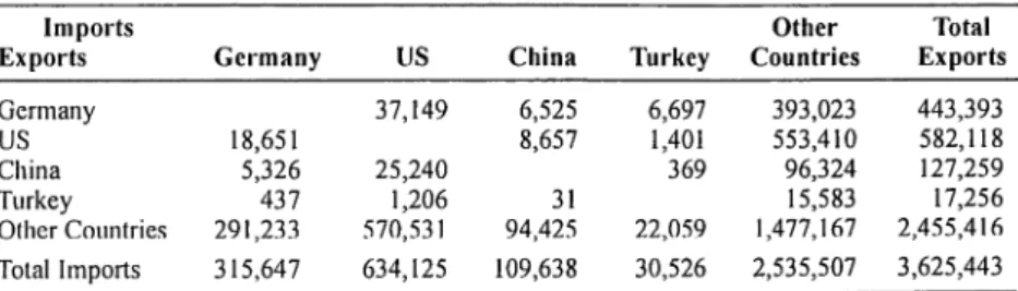
To study the problems related with the choice of weights, consider Table 1.1 Table 1.1a shows the manufacturing trade data for a sample of countries (Germany, the US, China, Turkey, and other countries) during 1996 obtained from foreign trade statistics provided by OECD on CD-ROM. Manufactures consist of the commodities SITC sections 5+6+7+8 minus divisions 68 and 891. From the table it follows that Germany has exported $37.1 billion to the US,
$6.5 billion to China, $6.7 billion to Turkey and $393 billion to the other
coun-tries making a total of $ 443.4 billion of German exports of manufactured goods. Germany has imported $18.7 billion from US, $5.3 billion from China,
$0.4 billion from Turkey and $291.2 billion from other countries making a total
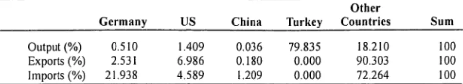
of $315.6 billion of German imports of manufactured commodities. Table 1.1b shows the value of domestic manufacturing production for the home markets of the four countries during 1996, where the value of domestic manufacturing pro-duction is determined as value added in the manufacturing sector minus the value of manufacturing exports. Table 1.1c puts the two types of data into one table where the column sum is defined as domestic absorption of the country under consideration. Table 1.1d shows the shares of the countries in domestic absorption. According to the table, German producers of import-competing commodities account for 76.88 percent of the German market. In the German market the share of US exporters is 1.37 percent, of Chinese exporters 0.39 per-cent and of Turkish exp01ters 0.03 perper-cent. Finally, Table 1.1e shows the shares of various countries in Turkish output, exports and imports. From the table it follows that exports to Germany account for 0.51 percent, exports to the US 1.409 percent, and exports to China 0.036 percent of Turkish output
Table 1.1: Calculation of Trade Weights
Table 1.1a: Manufacturing Trade of Selected Countries during 1996 (Million USS)
lm ports Other Total
Ex ports Germany US China Turkey Countries Exports
Germany 37,149 6,525 6,697 393,023 443,393 US. 18,651 8,657 1,401 553,410 582,118 China 5,326 25,240 369 96,324 127,259 Turkey 437 1,206 31 15,583 17,256 Other Countries 291,233 570,531 94,425 22,059 1,477,167 2,455,416 Total Imports 315,647 634,125 109,638 30,526 2,535,507 3,625,443
Table 1.1b: Domestic Manufacturing Production for Home Market of Selected Countries during 1996 (Million US$)
Other
Germany US China Turkey Countries
Germany 1,049,632 US 2,951,562 China 771,520 Turkey 68,319 15,150,640 Other Countries
Table 1.1e: Manufacturing Trade and Domestic Manufacturing Production for Home
Market of Selected Countries during 1996 (Million USS)
Other Total
Germany US China Turkey Countries Output
Germany 1,049,632 37,149 6,525 6,697 393,023 1,493,026 US 18,651 2,951,562 8,657 1,401 553,410 3,533,680 China 5,326 25,240 771 ,520 369 96,324 898,780 Turkey 437 1,206 31 68,319 15,583 85,576 Other Countries 291,233 570,531 94,425 22,059 15,150,640 16,128,889 Domestic Absorption 1,365,279 3,585,687 881,158 98,845 16,208,980 22,139,949 Table 1.1d: Share of the Country in Domestic Absorption (%)
Other
Germany US China Turkey Countries
Germany 76.88 1.04 0.74 6.78 2.42 US 1.37 82.32 0.98 1.42 3.41 China 0.39 0.70 87.56 0.37 0.59 Turkey 0.03 0.03 0.00 69.12 0.10 Other Countries 21.33 15.91 10.72 22.32 93.47 Sum 100 100 100 100 100
Sfibidey Togan
Table 1.1e: Share of the Country in Turkish Output, Exports and Imports
Other
Germany US China Turkey Countries Sum
Output (%) 0.510 1.409 0.036 79.835 18.210 100 Exports (%) 2.531 6.986 0.180 0.000 90.303 100 lrnports (%) 21.938 4.589 1.209 0.000 72.264 100
Source: Author .'s- calculations based on trade data/ram OECD and value added dalafrom UNIDO From Table 1.1 we note that Turkish manufacturing exports amounted to $ 17.256 billion where 2.531 percent of the total was exported to Germany, 6.986 percent to US, 0.18 percent to China and 90.303 percent to other coun-tries respectively. Considering these shares as weights of the competitiveness index one could construct an index of export competitiveness as:
’ a. (CPI /E)
;—
(CPI/E)
where 0Li denotes the share of country i in total exports under consideration, CPIi the consumer price index of country i, Ei the exchange rate of country i measured as domestic currency per unit of US dollars, CPI the consumer price index of the home country, E the exchange rate of the home country measured as domestic currency per unit of US dollar, and l the number of countries under consideration excluding Turkey. The case assumes that exporters of the home country face competition in foreign markets from domestic producers in the various markets. Alternatively, one could consider the competition that producers of import substitutes in Turkey face from the various foreign pro-ducers exporting to Turkey. Note that imports from Germany, US and China in total imports of $ 30.526 billion amounted to 21.938 percent from Germany, 4.589 percent from the US, 1.209 percent from China and 72.264 percent from the other countries. Using these shares as weights one could obtain an index of import competitiveness using a formula similar to that given above.
Durand, Simon and Webb (1992), Turner and Van’t dack (1993), and Zanello and Desruelle (1997) note that exporters face competition from both domestic producers and exporters from other countries. Thus, in the German market, Turkish producers have to compete not only with German producers but also with exporters from the US, China, and other countries. Data in Table 1.1d reveal that in Germany, German producers claim 76.88 percent of the market, against 1.37 percent supplied by the US, 0.39 percent supplied by China, 0.03-percent supplied by Turkey and 21.33 percent supplied by other countries. Likewise German exporters account for 1.04 percent, Chinese exporters for 0.7 percent, Turkish exporters for 0.03 percent and other
countries for 15.91 percent of the US market, the remainder being supplied by US producers.
The next step is to weight the different markets. This is done by calculat-ing the relative importance of the various markets to Turkish exporters. The German market accounts for 2.531 percent, the US market for 6.986 percent, the Chinese market for 0.18 percent and other countries for 90.303 percent of Turkish exports. Combining both steps would result in assigning a weight for
Germany in the Turkish export weighting scheme of some 26.4 percent
(0.02531 times 0.7688 [German market] plus 0.06986 times 0.0104 [US mar-ket] plus 0.0018 times 0.0074 [Chinese marmar-ket] plus 0.90303 times 0.0242 [the market of other countries]).
Overall trade weights are derived by combining the bilateral import weights with the double export weights, using the relative Size of Turkish imports and exports in overall Turkish trade to average both sets of weights. Turner and Van’t dack (1993) put these in formal terms as:
Import weight: w,” = (M, / M ) Ark
y,+ZX,’
;(X) y,+Z./;X
. M m X x Overall weight: w, = w, + w, X + M X + Mwhere Mi denotes imports of the home country (Turkey) from country i, M
total value of Turkish imports, Xi Turkish exports to country i, X total value
of Turkish exports, yi value of domestic manufacturing production for home market of country i, and X"i exports of country k to country i.
On the other hand, Zanello and Desruelle (1997) denote by Tij the (i,j)-th element of a table similar to Table 1.1c. They assume that, including the home
country, there are n countries. The shares of the countries in domestic
absorp-tion similar to those shown in Table 1.1d are denoted by 3,2 0 (i,j=1,..,n). For purposes of exposition they order the countries so that the home country is the n-th country. Note that by construction we have:
23,, :1
(i=l ,..n)
i=l
For j 75 n let v,,,-= (T,,,-/ E T,,,-) be the share of Turkish exports to country j
in total Turkish manufacturing output and for j = n let v,,,, = (T,,,,/ j T,,,-) j = l
Silbidey Togan
be the share of Turkish domestic manufacturing production for the home
mar-ket in total Turkish manufacturing output where:
z = I.
.l'Zanello and Desruelle (1997) determine the share of country i and show that this value equals the overall weight of Turner and Van’t dack (1993):
)3
fl = ————’='
i n-lZ vnk (.1 _Snlr ) k=l
Finally, turning to the question of mathematical formulation of the index we note from Vartia and Vartia (1984) that the issue of the mathematical for-mulation of the index has been largely resolved in favor of geometric averag-ing. As a result, Zanello and Desruelle (1997) use the formula:
) I
u/ ‘5";
RER = n CPI,/ E,
CPI/E
where i is the index that runs over the country’s trade partners, and wi the com-petitiveness weight attached by the country to country i.
3. CPI-Based and ULC-Based Real Effective Exchange Rates
Equipped with the methodology described above, the competitiveness
indica-tors for the MENA countries consisting of Egypt, Morocco, Tunisia and
Turkey are determined as follows. We consider as competitors of the MENA countries and as major suppliers of imported commodities to the MENA countries the following countries in four groups:
0 Western Europe: Belgium, France, Germany, Greece, Italy, Netherlands,
Portugal, Spain, Switzerland, and UK
America: Brazil, Canada, Mexico, and the US
Central and Eastern European and Commonwealth of Independent States Countries: Czech Republic, Hungary, Poland, Russia
0 Asia: China, Indonesia, Japan, Korea, Malaysia, Taiwan, Thailand
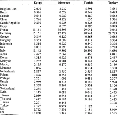
In the following we abstract from consideration of the other countries and concentrate on the year 1996. To determine the weights wi of these countries we need data similar to those of Table 1.1c, i.e. data on manufacturing exports to and imports from the countries under consideration to each of the other countries as well as data on gross manufacturing output of the 29 countries (four MENA countries, ten West European countries, four countries in
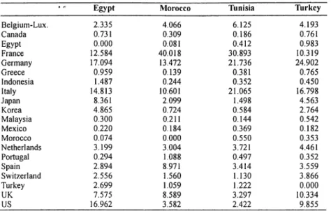
America, four CEE and CIS countries, and seven Asian countries) under con-sideration. The trade data are obtained from the OECD trade data on CD-ROM supplemented by United Nation Comtrade data. For gross output of the manufacturing sector we use the OECD STAN database and industrial data provided by UNIDO. This exercise requires that we fill in all the entries in the 29x29 matrix. Monthly CPI and exchange rate data for the countries under consideration over the period 1980—98 are obtained from two sources: IMF International Financial Statistics CD-ROM and data provided by Datastream. Table 1.2 shows the trade weights used in the calculations. Two sets of weights are used in the calculations. Thefirst set consists of 20 countries and is shown’ in Table 1.2b. The second set of weights is shown in Table 1.2a. The first set excludes the former communist block countries as well as countries with very high inflation rates such as Brazil. These weights have been used for the period 1980—95. The larger set of weights have been used for the peri-od 1996—2001.
Table 1.2a: Trade Weights of MENA Countries during 1996—99
Egypt Morocco Tunisia Turkey
Belgium-Lux. 2.070 3.737 5.891 3.651 Brazil 0.526 0.629 0.349 0.493 Canada 0.648 0.289 0.180 0.662 China 3.296 4.228 1.035 1.326 Czech Republic 0.830 0.228 0.425 0.386 Egypt - 0.075 0.396 0.849 France 11.161 36.893 29.941 9.043 Germany 15.151 12.422 20.941 21.783 Greece 0.849 0.129 0.368 0.665 Hungary 0.363 0.089 0.117 0.334 Indonesia 1.316 0.229 0.340 0.396 Iran 0.001 0.390 0.349 0.778 Italy 13.142 9.802 20.392 14.680 Japan 7.422 2.062 1.466 4.041 Korea 4.315 0.729 0.578 2.457 Malaysia 0.267 0.204 0.141 0.464 Mexico 0.195 0.170 0.359 0.159 Morocco 0.066 - 0.534 0.308 Netherlands 2.827 2.750 3.559 3.857 Poland 0.426 0.351 0.263 0.810 Portugal 0.261 1.001 0.481 0.307 Russia 2.959 0.333 0.140 5.998 Spain 2.568 8.269 3.308 3.106 Switzerland 2.264 1.445 1.096 3.370
Syria
0.143
0.081
0.041
0.473
Taiwan
2.039
0.645
0.414
1.347
Thailand 0.472 0.162 0.186 0.413 Tumsm 0.291 0.442 - 0.308 Turkey 2.397 0.979 1.182 -UK 6.712 7.894 3.181 8.979 US 15.020 3.345 2.346 8.555 13Su'bidey Togan
Table 1.2b: Trade Weights of MENA Countries during 1980—95
' " Egypt Morocco Tunisia Turkey
Belgium-Lux. 2.335 4.066 6.125 4.193 Canada 0.731 0.309 0.186 0.761 Egypt 0.000 0.081 0.412 0.983 France 12.584 40.018 30.893 10.319 Germany 17.094 13.472 21.736 24.902 Greece 0.959 0.139 0.381 0.765 Indonesia 1.487 0.244 0.352 0.450 Italy 14.813 10.601 21.065 16.798 Japan 8.361 2.099 1.498 4.563 Korea 4.865 0.724 0.584 2.764 Malaysia 0.300 0.211 0.144 0.542 Mexico 0.220 0.184 0.369 0.182 Morocco 0.074 0.000 0.550 0.353 Netherlands 3.199 3.004 3.721 4.461 Portugal 0.294 1.088 0.497 0.352 Spain 2.894 8.971 3.414 3.559 Switzerland 2.556 1.560 1.130 3.866 Turkey 2.699 1.059 1.222 0.000 UK 7.575 8.589 3.297 10.334 US 16.962 3.582 2.422 9.855
Source: Author 19 calculations
Figures 1.1-1.4 present estimates of CPI-based real effective exchange rate indices for the MENA countries over the period 1980-2001. But these estimates turn out to be problematic mainly because of the particular charac-teristics of the MENA countries’ exchange rate regimes explained below in more detail.
Egypt: In Egypt during the 1980’s there were three rates of foreign
exchange (Mongardini [1998]). The first rate was that of the Central Bank
which was keptfixed at 0.7 L.E/US$ from 1979 until 1989 when it was
reval-ued to 1.1, and to 2 LE/US$ in 1990. The central bank rate was used for exports of petroleum, cotton, rice, Suez canal dues, and imports of essential
foodstuffs. The second rate was the commercial banks’ rate initiallyfixed at
0.83 L.E./US$ in 1982. It continued to be devalued until its abolishment in 1989. This rate was used for worker remittances and tourism. Both rates were marked by heavy intervention. In addition, foreign exchange was traded at a premium rate in a non-bank free market. In this market, which was formally illegal but officially tolerated, the exchange rate was negotiated by the parties to the transaction. During the first half of 1980’s Egypt faced pressures from its balance of trade, as well as from current account imbalances, due to the precipitous fall in oil prices and consequently in the related sources of foreign exchange, i.e. Suez Canal tolls and workers’ remittances. Nevertheless, the exchange rate was not actively used to restore external equilibrium, and
instead the government resorted to imposing restrictions. This was probably due to the usual fear that currency devaluation would fuel inflation.
In May 1987 a new bank foreign exchange market was allowed. The sec-ond foreign exchange rate mentioned above ceased to exist by 1989. In the new market, resources were drawn from worker remittances, tourist expendi--tures, and specified export earnings. The new market was permitted to provide foreign exchange mainly for private sector imports. Other transactions were
required to befinanced through the central bank pool.
In February 1991, the old multiplefixed parity exchange system was
abol-ished, and replaced temporarily by a dualflexible peg exchange rate system.
In October 1991, for thefirst time in decades in Egypt, segmented markets for foreign exchange were unified at a value guided by the market forces. The nominal exchange rate was revalued by 23 percent and became convertible for current account transactions. Buying and selling foreign currencies, upon obtaining proper licensing, was allowed outside the banking system. In June 1994 the foreign exchange market was further liberalized by easing capital account restrictions. During this period the nominal exchange rate of the Egyptian pound vis-a-vis the US dollar, being used as a nominal anchor, was roughly constant.
Figure 1.1: Real Exchange Rate of Egypt
140 120- 100- 80-60— Real Exchange Rate (RER) of Egypt 40-20 80 82 84 86 88 9O 92 94 96 98 00 Years RER of Egypt
Sfibidey Togan
Regarding the evolution of the real exchange rate in Egypt, we note from Figure 1.1 that the real exchange rate appreciated during the 19803 until 1990.
The real exchange rate depreciated considerably during 1990—91, but
there-after it started to appreciate again.
Morocco: During the 19703 Morocco’s macroeconomic performance was steadily deteriorating. The authorities reacted by tightening restrictions on trade and payments. This policy of tightening restrictions was reversed in the mid-19803 and regained momentum in the early 19903 (Nsouli et al. [1995]). During this period, current account liberalization proceeded in parallel with trade reform. The main measures taken were the gradual reduction and final-ly abolition in 1984 of import deposit requirements, the abolishment of the listed import schcme in April 1985 under which imports required a license, and the elimination of the requirement of approval from the Moroccan Exchange Office for payments on imports of specified list of goods. A further reduction in restrictions took place in November 1985 when maximum customs duties were reduced to 45 percent and special import duties to 5 percent.
A new foreign trade code was passed in 1991 simplifying regulations and confirming Morocco’s commitments to a liberal trading system. Liberalization of inward and outward investment involving nonresidents start-ed with the reform of the investment code in 1983. The code was further lib-eralized in 1988, and in 1992 the repatriation of profits and capital from foreign investment was virtually fully liberalized. In 1991, export promotion accounts in convertible dirhams were introduced, allowing exporters to retain the dirham equivalent of part of their exchange proceeds in such accounts to be used for certain business related to expenses abroad. In 1993, exporters were allowed to retain a portion of their foreign exchange proceeds in foreign exchange accounts with domestic banks, and in late 1993 foreign borrowing
by domestic firms for most purposes was liberalized. By the end of 1993,
Morocco had established, besides convertibility on current accounts, full capital account convertibility for foreign investors.
During the 19803 the nominal exchange rate was set on the basis of a currency basket that comprised the currencies of Morocco’s principle trading partners. Under this system the authorities pursued an active exchange rate policy during 1980—86 to depreciate the dirham gradually in real terms. Figure 1.3 reveals that the authorities have been successful in their attempts. The balance of payments pressures in 1990 forced a devaluation of the dirham by 9.25 percent against the basket of currencies to which the currency was pegged. Subsequently the dirham was pegged against the basket and the real exchange rate started to appreciate. A major step toward liberalizing the foreign exchange market was taken in 1996 when the interbank market for foreign exchange was established. But the Bank of al-Magrib (central bank)
still played a dominant role in the foreign exchange market. The bank set daily rates for major currencies, determined according to a currency basket in which the French franc predominated. The link with the franc led to the real appreciation of the exchange rate observed during the 19903.
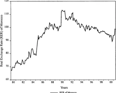
Figure 1.2: Real Exchange Rate of Morocco
120 HQ. 100- 80-Real Exchange Rate (RER) of Morocco 8 L 70-60 80' '32' '34' '86' '38' '90' '92' '94' T96, '98' '00' Years RERofMorocco
Regarding the evolution of the real exchange rate in Morocco we note from
Figure 1.2 that the real exchange rate depreciated during the period 1980—93, and thereafter appreciated rather slowly over the period 1993—2001.
Tunisia: During the 19803 the Tunisian dinar was linked to a basket comprising the French franc, German mark, US dollar, Italian lira, Belgian
franc, Dutchflorin, and the Spanish peseta (Domac and Shabsigh 1999). But
the link was not effective in eliminating the mid-19803" pressure on the dinar caused by the recession and balance of payments problems. In response the authorities started to depreciate the dinar until early 1989. The depreciation of the dinar coupled with the economic reform program in late 1980’s and early 1990s stabilized the foreign exchange market. Toward the end of 1992, the exchange rate was liberalized for current account purposes (Nsouli et al.
1993). The government scrapped exchange controls from January 1993,
making the dinar also convertible for foreign investors for repatriation of cap-ital or profits. Private individuals and firms were allowed to open foreign cur— rency accounts, and the government eased the transfer of funds abroad, but
Sz'ibidey Togan
eign exchange transactions were still kept at the central bank. The interbank
foreign exchange market was established during 1994, allowing banks to trade
foreign currency at more flexible rates. During the period 1988—89 the central
bank took additional measures for capital account liberalization, resident enterprises being allowed to keep up to 50 percent of their export proceeds and up to 50 percent of the proceeds of their borrowing abroad in foreign curren-cy deposits. Nonresidents have been allowed to buy shares of Tunisian com-panies provided that total share of foreign participation does not go beyond a ceiling of 50 percent.
The exchange rate policy in Tunisia has been guided by a real exchange rate objective based on a basket of competitor and partner countries, but infor-mation on the basket is not disclosed. Regarding the evolution of the real exchange rate in Tunisia we note that the policy has been successful. As shown in Figure 1.3 the real exchange rate has fluctuated within a relatively narrow margin over the period 1987—99. The real exchange rate has depreci-ated slightly from 1987 until mid 1991, apprecidepreci-ated rather slowly over the period 1991—99, and depreciated again slightly after 1999.
Figure 1.3: Real Exchange Rate of Tunisia
106 oA l ON l 1004 Real Exchange Rate (RER) of Tunisia \0 W l 96 88 89 90 91 92 93 94 95 96 97 98 99 00 01 Years RER of Tunisia
Turkey: Toward the end of the 1970s, Turkey followed a fixed and multi-ple exchange rate policy. With the stabilization measures of 1980, Turkey devalued the Turkish lira by 33 percent in January 1980, and eliminated the
multiple exchange rate system except for imports of fertilizers and fertilizer inputs. After May 1981 the exchange rate was adjusted daily against major currencies in order to maintain the competitiveness of Turkish exports. Multiple-currency practices were phased out and bilateral payments agree-ments with non-Fund members were terminated during the first couple of years of the 1980 stabilization program. In January 1984, domestic commer-cial banks were allowed to engage in foreign exchange operations within cer-tain limits, and restrictions on foreign travel and investment from abroad were eased and simplified.
Theflexible determination of the exchange rate was further liberalized by
permitting banks to set their own rates within a specified band around the Central Bank rate. The policy led to depreciation of the real exchange rate over the period 1980—88 as revealed by Figure 1.4. In August 1988 major reform was introduced and a system of market setting of foreign exchange rates was adopted. But with the real depreciation of the Turkish currency, real wages started to decline. By the second half of the 19805 popular support for the government had started to fall off. In the local elections of March 1989, the governing political party suffered heavy losses. To increase political sup-port the government conceded substantial pay increases during collective bar-gaining in the public sector during 1989. Consequently, pressure built up in the private sector to arrive at similarly high wage settlements. As a result of these developments the real wages started to increase and simultaneously the real exchange rate appreciated. The increase in real wages was not sustain-able. In 1994 the country faced balance of payments crises. With the intro-duction of stabilization measures, the trend in real wages was reversed. Real wages started to decrease and the real exchange rate to depreciate. But because of relatively weak coalition governments, the country had to reverse its economic policies. The appreciation of the Turkish Lira carried on until the end of 1999 when the country was forced to sign a stand-by agreement with the IMF.
At the end of 1999 Turkey embarked upon an ambitious stabilization program, aimed at achieving single digit inflation by 2002. The policy of a pre-determined exchange-rate path as a nominal anchor in an inflationary environment led to considerable real exchange rate appreciation. A severe banking crisis blew up in November 2000, accompanied by massive capital
outflow. An IMF-led emergency package has succeeded for a while in
nor-malizing the situation. Developments in February 2001 led to a total loss of confidence in the government’s program and a serious run on the Turkish lira. Interest rates skyrocketed and foreign exchange reserves started to decline rapidly. The government decided to abandon the crawling peg regime. The
currency was floated. As a result, the exchange rate depreciated sharply. A
Sfibidey Togan
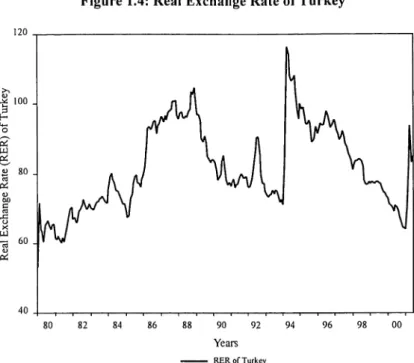
Figure 1.4: Real Exchange Rate of Turkey
l20 O O l Real Exchange Rate (RER) of Turkey 0\ 00 O O l l 4O I I I I I j I 1 *I I I l I I I I I 80 82 84 86 88 90 92 94 96 98 00 Years RER of Turkey
Regarding the evolution of the real exchange rate in Turkey, we note from Figure 1.4 that the real exchange rate has depreciated during the period 1980—89, appreciated during the period 1989—93, depreciated rather sharply during the crises period of 1994, appreciated over the period 1994 until February 2001, and depreciated sharply thereafter.
Table 1.3 presents the coefficient of variation (standard deviation divided by the mean) for the MENA countries. The table shows that the effective real exchange rate has been relatively less volatile in Tunisia and Morocco.
Table 1.3: Coefficient of Variation of Real Effective Exchange Rates
Egypt Morocco Tunisia Turkey
0.4207 0.1320 0.0227 0.1435
Source: A utlmr Iv calculations.
As the discussion of exchange rate policies followed by MENA countries reveals the real exchange rate series obtained for those countries face prob-lems. The main problem with the estimates is the fact that most of these coun-tries have introduced multiple exchange rates over certain parts of the period 1980—99. Since the estimates given above were obtained using the exchange rate series provided by IFS, the estimates do not take into account the
plexities introduced by multiple exchange rates. A more satisfactory approach would be to obtain separate time series of multiple exchange rates for each MENA country and then weight these series for each country with their rele-vant market shares to obtain a single weighted average exchange rate series over the period 1980-99. But because of data limitations this approach could not be followed. Furthermore we note that the CPI includes non-traded goods as well as traded goods. If traded and non-traded prices diverge over time, aggregate price indices could be misleading indicators of the prices of traded goods. In addition CPI’s are endogenous to the exchange rate since they include import prices, and therefore understate changes in competitiveness.
On the other hand, the unit labor costs (labor cost per unit of output) cap-ture a key element of competitiveness. By focusing on costs rather than prices, unit labor costs avoid some of the endogeneity problems of the CPI. But unit labor costs have a major limitation: data on labor productivity and labor com-pensation are not always reliable or available on a timely basis. The calcula-tions are obtained using the formula:
RER=H[C’/ E]
C/ E
where Ci denotes the unit labor cost in country i measured in terms of i-th coun-try’s domestic currency, Ei the exchange rate of country i, C the unit labor cost of the home country, and E the exchange rate of the home country.
In the following calculations the data come from three sources. These are the US Department of Labor (2000), OECD (1999), and UNIDO data. The unit labor cost figures for Belgium, Canada, France, Germany, Italy, Japan, Korea, Netherlands, Taiwan, the United Kingdom, and the US have been obtained from the US Department of Labor (2000) for the period 1980—88. The STAN OECD database (1999) provides figures for manufacturing value added at con-stant prices, labor compensation and employment over the period 1980—97. Here, productivity is obtained by dividing value added at constant prices by employment and wage is determined as total earnings of labor divided by employment. Unit labor cost is then calculated as compensation per employee divided by productivity. The STAN database has been used to obtain the unit
labor cost figures for Greece, Portugal and Spain. Other data come from the
United Nations Industrial Development Organization (UNIDO) Industrial Statistics database, obtained on disc from UNIDO, supplemented with manu-facturing value added deflators from the World Bank. The UNIDO database provides manufacturing value added at current prices, labor compensation and employment. Productivity is obtained by dividing value added by employment,
and deflating the figures with the World Bank (2000) manufacturing
value-added deflators. Finally, data on manufacturing value added, labor
Siibidey Togan
tion, and employment for Turkey has been obtained from the Statistical Institute of Turkey and data for Egypt from Cottenet and Mulder (2000).
Table 1.4: Real Exchange Rates Based on Unit Labor
Cost Figures
Egypt Turkey 1980 66.72 66.85 1981 63.00 60.84 1982 61.03 58.56 1983 58.28 55.55 1984 54.81 51.66 1985 54.49 51.40 1986 66.77 65.45 1987 77.15 77.68 1988 80.90 81.22 1989 80.47 78.61 1990 91.35 90.71 1991 94.78 93.49 1992 100.00 100.00 1993 96.07 94.12 1994 94.57 93.34 1995 100.77 100.52 1996 100.07 100.58 1997 90.72 90.71Source: Author .'s' Calculations
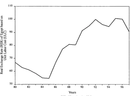
Figure 1.5: Real Exchange Rate of Egypt based on Unit Labor Cost
110 100 _ \O O l 80.. 70-60.1 Real Exchange Rate (RER) of Egypt based on Unit Labor Cost (ULC) 50 30 82 84 86 ' 3's ' 9b ' 9'2 ' 9'4 96 Years
RISR 01‘ Egypt based on ULC
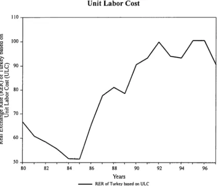
Figure 1.6: Real Exchange Rate of Turkey based on Unit Labor Cost
110 100 — \O O l 80 -70-4 Real Exchange Rate (RER) of Turkey based on Unit Labor Cost (ULC) 60-50 80 82 84 86 88 90 92 94 96 Years
RER of Turkey based on ULC
In the following, we report the real exchange ratefigures for only Egypt and Turkey as there are too many missing observations for the other countries. Table 1.4 and Figure 1.5 show that the real exchange rate based on unit labor costs in Egypt appreciated during the period 1980—85, depreciated thereafter until 1996 and started to appreciate again in 1997. On the other hand, Table 1.4 and Figure 1.6 show that the real exchange rate based on unit labor cost in Turkey depreci-ated during 1980-1985, and apprecidepreci-ated during 1985—93. The real exchange rate depreciated in 1994, appreciated until 1996 and depreciated again 1997. 4. Other Indices of Competitiveness
The focus of this section will be on some of the indicators used in analyzing industrial competitiveness at the sectoral level. We concentrate on measures of comparative advantage. The first measure considered is the index values of revealed comparative advantage (RCA) defined as:
(XMX)
RCA,=ln(W_)_) ,
where Xi denotes export of commodity i by the country considered, X total exports of the country considered, Xi‘vorld total world imports of commodity i and
Subidey Togarz
X‘”°"d total world imports. The equation considers the share of commodity i in the total exports of the country relative to the share of the commodity i by the world to total world imports. In general, if this ratio is greater than one, then the natur-al logarithm of the variable will be positive. In that case the country is said to have a comparative advantage in producing that product. Using the index of revealed comparative advantage, it is possible to determine which product cate-gories each of the MENA countries have the greatest comparative advantage. Table 1.5 shows the 22 sectors with RCA values in 1996. The table reveals that MENA countries have comparative advantage in the following sectors:
- Egypt: Fuels, textiles, clothing, non-ferrous metals, and agricultural raw
materials.
- Morocco: Inorganic chemicals, clothing, ores and other minerals, food, and
other chemicals.
- Tunisia: Clothing, inorganic chemicals, other chemicals, electrical machin-ery and apparatus, fuels, ores and other minerals, and textiles.
- Turkey: Clothing, textiles, iron and steel, food, ores and other minerals, and inorganic chemicals.
A related measure of comparative advantage is based on market shares in major markets. Since the major market for MENA countries is the European Union we consider the market share of MENA countries in European industri-alized countries. Table 1.6, showing the market shares of the MENA countries, reveals that the three commodities with highest market shares are fuels, textiles, and non-ferrous metals in Egypt; clothing, inorganic chemicals, and ores and other minerals in Morocco; clothing, inorganic chemicals, and electrical machinery and apparatus in Tunisia; and clothing, textiles, and ores and other minerals in Turkey
A third measure of comparative advantage considers the sectors with increasing market shares. Among these sectors the dynamic sectors are defined to be those sectors with growth rate of exports exceeding the growth rate of imports in the export markets. For the MENA countries the dynamic sectors with increasing market shares are:
- Egypt: Plastics, pharmaceuticals, other chemicals, power-generating
machinery, other non-electrical machinery, and other consumer goods.
- Morocco: Organic chemicals, plastics, power-generating machinery, other
non-electrical machinery, office machines and telecommunications equip-ment, electrical machinery and apparatus, and other consumer goods.
- Tunisia: Plastics, pharmaceuticals, power-generating machinery, other
non-electrical machinery, office machines and telecommunications equipment, electrical machinery and apparatus, and other consumer goods.
- Turkey: Pharmaceuticals, power generating machinery, other non-electrical
machinery, electrical machinery and apparatus, and other consumer goods.
30.23338 M .853». 623% The Changing Pattern of Competitiveness in MENA Countries 3.5 m5.5 mmd find 86 4350.5 mm5md-02m.” w5om.- NmO5d-wwh 3.2 mod-55.? mod mauscohm .550 5w+o T mmmm. 82;- 386- mT 8.5 3.3 3.2 mNd— Sdm mnooO 583200 550 Sw-ow-vm-m Hmmmd mvN 35:5. Goad mad mmd 2.2 mod oZN matte—U Vw 33.? ooood mwmmg 53; 86 556 53: mod-vo.5 8:385 we mm_5+wm _5 +mm_5+_m #5 mmd T 3%. 089m- mmm5.T 83.0. 3.2 3.5-vd $.5T EoEaEcm top-$98.5 850 +ow5+mw5+m5 mw55+m25 33¢- 3w¢.m- wvo5.m- own:-wod m5.5N mm; m _.m-3.3 8260i u>toEoS< +ow5-mm5-w5 mBmHmaa< omfimd-oocmd m5wod-5% ”.m-mo. 2 5.3 no.9 modm mod 23 53:2a Rom-zoom” 355655-55 EoEnEcm vm5_.m- vwgwd- oommd- mmé-50.2 omé 5md 3.: mwd .3... Ed 3:282 350 o55+o5+m5 @3582 ovG. T mmmm.- 85:”- ommod-3.5 mmd. 50.2 5V4“ 50d 185020-52 EEO V5+m5+m5 mE buEfi ooRd-5vow. T mNNm.N-39.6. m a.5 mm. E Now 2.5 w fl.Nm mcufi ocoo 526m EoEaScm m 5-5 “-53:85 U5 55:583— 53Nd- motto-O52. T O5mm.T V5.0 502 m #6 3.9 wwdm muBHummscmE-mfiom $50 3-50-3-0 w5m5d cwmw.T m5mcd mowed-~5.5 _5._ NZ. mod-02: mfiomEuno .550
mm+om+mm+mm m5.m_ Nmmad- mmomd- 350m-
momfim-Elm $3 a; 52% 23.558255 3 Newmd m5oo.m . V5506 5m5m.o-m5.m $5 V5.5 Nvd ema— mfiofi cono £5905 mm vmw w5¢m.m- «www.m- owmmN- 33;. mod mow vod 5v.: 8.5m wm+5m mwmo.v- Some. 834- m5mfim-wm.m cod- no.9-m5.N_ mm.m-WEBB-EU 35t fim fiono fluom No2; ow?!- 5owo.m- 5506-cod v9: 3.: woe 59: 3o can so: 50 8:38:52 mommd- good- $36-m5ovd Vma w5._ 3.2 5nd 2. T 292: Setup-:02 mo _w5m.m- 32.0 w5owT mama; 5m.~ $.3- moN- mod-mad 225 m vd- $o 336 5owm.o 8; mm; ow.m 2;-$5 28052 550 use WBO wm+5m 9:52 32695 856-comm. T m5mmd-356 SM N: 5.6 36 _m.m mECoEE 3mm _E=:=o_._m<
wm-5m-mm-m vmmod- Svo; 053d- good
Ewe :.m $4.” 96 m5.m_ noom mm+v+ To _a._3_=u_._w< $2695 33 :2 3.: 3.: 33-82 5:: «Es: 883: 33m 32-82 $2.82 waaéa ”tas— 33.... 8832 225:. 32:: 33-8.: $85.56
8.5 .3 mtoaxm .3 mtoaxm ..o 339nm— .3 33a .3 2.53 ownu=a>u< ouuuza>u< mus—53:... eunuca>c<
033.3955 gains—Eco grahaafi ou 9:223:80 23— 539.0 3am 5.59.0 3am EBEU 8am 539.0 35— 539.0 25
Su’bidey
Togan
#:0223360 w. Loin—x 50.50% a—<.—.O.—. 050:.0 000—0 0000 0000.0 0000.0 0050 0000.0 3000 32.00.:— 550 —00+0 0000.0 —00—.0 000—0 0530 000 —.0 0050.0 0000.0 50—00 380 553—50 5:00 0000400 00 _ 0.0 00.000 000 0.0 5000.0 030.0 000 _.0 00.500 30 —.0 05:55 00 5000.0 0000.0 0000 000—0 5300 0000.0 300.0 05000 5:380. 00 00_5+00 :5 +00 _5 +_ 0_5 5000.0 000 _.0 0000.0 0000.0 0000 05—00 0000.0 0_0—0 25235000 teams—E. 5:5 +005+005+0 0055+00 :5 0000.0 0000 3—00 05—00 0000.0 030.0 0000.0 300.0 32680 0355930 +005-005-05 355090 00000 005—0 0000.0 0000.0 005—0 2500 0v000 5000.0 0:5 b.5552 52.520— 0055-055-55 000:0 000—0 0080 05—00 V520 0050.0 0000.0 0000.0 EofinEcm— 50. .0. 35:52 00000 055+05+05 00:0 0000 0000.0 —0000 50 —0.0 00—00 00 —00 00—00 055552 52.555-207— 550 V5+05+05 030.0 —0000 0300 0:00 500.0 0000.0 000—0 0000.0 055552 0:55:50 5300 05.5 EoEmScm tam—5C. 05 05.5552 5000.0 0000.0 000.0 050.0 0000.0 5500.0 005.0 0000.0 508505524550 5:00 00-50000 00v00 :0500 300.0 0000.0 503.0 0000.0 0000.0 0000.0 2855.6 5:00 00+00+00+00 . 0 _ 00.0 #0000 0000.0 0 000.0 _000.0 0000.0 5 _ _0.0 5000.0 mfiucauom fimi 00 5005.0 0500.0 0050.0 0500.0 0000.: 0000.0 0000.0 5000 280.5:0 0:505:— 00 00— —.0 003 .0 0 80.0 0000.0 030.0 0 _ 00.0 0000.0 0000.0 3:55 00+50 000—0 0000 0000.0 _000.0 0000.0 0500 0000.0 0000.0 2:355:00 0050.5 :0 $5255.00 0000.0 0000.0 200.0 0000.0 5000.0 0000.0 0000.0 000—0 580 05 so: 50 8:550:52 0000.0 000.0 0000.0 0000.0 000.0 050—0 0000.0 :30 £555 38.50.52 00 0030 0000.0 0000.0 0000.0 V0000 5000 0005.: 5500.: £050 0 0000: .310.— 00000 000..0 _000.— 0000.: 002.0 0000.0 25552 5:00 0.5 5:0 00+50 0552 32:5...”— 0000 0000.0 00¢00 5000.0 0— .00 000—0 055—0 0030 m5552 25¢ _m._=::otm< 00-50000 300.0 0000.0 20 —.0 0500.0 0000.0 0 _ 00.0 00_ —.0 0050.0 000... 00+v+_+0 5._:::u_._0< 95:09.0 000— 000— 000— 000— 000— 000— 000— 000— 95:0 95:0 95:0 95:0 95:0 95:m 95:0 95:0 oEEoU 05—0 5552 5:52 5:52 5:52 50.52 50.52 5:52 50.52 5.3.5.0 525.0 .5553. 53:3. 55952 55952 530000— 5:000...—35955
3.80::
525.50—
:5595
E
00950—
535?»
3
359?..—
<Zm2
.5
95:0
50.52
”0.—
2:50.
26
5. Real Exchange Rates and Export Performance
Consider the export demand and supply functions of Goldstein and Khan (1985) shown below:
1 t’
lnxd =aq,+a,lnyf —a21n pig—T;f 1+ E
lnx, =fl,+fllny+fi,ln m
where xd denotes the quantity of the home country exports demanded by the rest of thc world, yr foreign real 1ncome, p foreign price of exportables, t tar-iff rate in the 1est of the world applied to imports from the home country, p* foreign price of goods produced in the rest of the world, xs quantity of home country exportables supplied, y the level of domestic real income, 5 the export subsidy rate applied by the home country, E the exchange rate defined as the price of foreign currency in terms of domestic currency and p the price of domestically produced goods. In the model, the first equation represents the quantity demanded as an increasing function of the level of real income in the importing region and as a decreasing function of the price of the imported good’s domestic price, inclusive of tariffs relative to the price of domestic substitutes in the rest of the world. The second equation indicates that the sup-ply of exportables depends positively on both the real income in the home country and the domestic price of exportables inclusive of export subsidies relative to domestic prices. Export supply is assumed to rise as the real income serving the purpose of an index of productive capacity of the home country rises. Furthermore, as the domestic price of exportables rises relative to domestic prices, production of exports will become more profitable and export supply will increase. The model, consisting of three equations, deter-mines the equ1l1b11um values of xd ,x ,and p for given values of the exoge-neous variables y, y, p, p* , t ,s dand E. Setting xd ——x ——x the solution for x can be expressed as:
Inx=(“°"2;“2
fl°)+(a;“)Wflw +(———Ji—l
where B= (22.oc+B) The reduced form equation reveals that exports increase
with increases in productive capacity of the country, increases in foreign real
income, and increases in the subsidy and tariff adjusted real exchange rate
[M
p(1+z/)
Siibidey Togcm
Empirical estimation of the export function faces a set of problems. We approximate the productive capacity of the country by the real GDP of the country. The foreign real income variable is calculated as the real GDP in the main export markets. The estimation of the export function for Turkey yields the relation:
In x = -39.382 +1.1431n y + 2.021 In yf+ 0.423111 RER
(-3.666)
(1.537)
(1.785)
(1.639)
1980 - 1999; n = 19; p = 0.207 ; R2 = 0.98; DW = 2.476
(0.1.529)
where x denotes Turkish exports from the manufacturing sector measured in terms of US$ and deflated by the US manufacturing sector value added defla-tor. The RER is the annual real exchange rate variable obtained above in Section 3 as monthly series for Turkey. The equation shows that all variables have the expected signs. An increase in domestic GDP, an increase in foreign GDP, and a depreciation of the real exchange rate leads to an increase in exports of the manufacturing sector.
On the other hand, difficulties were encountered when trying to obtain mates ofthe export functions for the other MENA countries. Least square esti-mates revealed that the export function does in general not have the correct signs for all ofthe three variables: real GDP, real GDP in the rest ofthe world, and real exchange rate. The reason may lie in the fact that these countries at various times during the period 1980—99 had introduced multiple exchange
rates and exchange controls, and the real exchange rate series used in the
cal-culations above did not take into account the complexities introduced by these restrictions. As a result the export functions for these countries did not yield satisfactory results.
6. Conclusion
This chapter has provided an overview of the concept of competitiveness and evidence on competitiveness trends in MENA countries. Narrowing the con-cept of competitiveness to countries’ ability to sell their products in world mar-kets, we have concentrated on real exchange rates and have shown that the real exchange rate depends on relative unit labor costs measured in terms of for-eign currency and relative profit margins. An increase in unit labor cost or profit margin relative to that in the rest of the world leads to deterioration of competitiveness. Consideration of the trends in real effective exchange rates
revealed that these rates have fluctuated considerably in Egypt, Turkey and
Morocco over the period 1980—99 and that it has been relatively stable in
Tunisia. It turns out that the type of exchange regime is of importance for the real exchange rate to affect exports. In countries with exchange controls and multiple exchange rates it is relatively difficult to determine a positive relation between export performance and real effective exchange rates based on monthly exchange rate and CPI indices of IFS. On the other hand in the case of Turkey, a country with a liberal exchange regime, a positive relation exists between export performance and real effective exchange rates.