AUTOMATIC RADAR ANTENNA SCAN
ANALYSIS IN ELECTRONIC WARFARE
a thesis
submitted to the department of electrical and
electronics engineering
and the institute of engineering and science
of bilkent university
in partial fulfillment of the requirements
for the degree of
master of science
By
Bahaeddin Eravcı
August 2010
Prof. Dr. Billur Barshan (Advisor)
I certify that I have read this thesis and that in my opinion it is fully adequate, in scope and in quality, as a thesis for the degree of Master of Science.
Asst. Prof. Dr. Sinan Gezici
I certify that I have read this thesis and that in my opinion it is fully adequate, in scope and in quality, as a thesis for the degree of Master of Science.
Asst. Prof. Dr. Yakup ¨Ozkazan¸c
Approved for the Institute of Engineering and Science:
L. Onural
Director of the Institute
ABSTRACT
AUTOMATIC RADAR ANTENNA SCAN
ANALYSIS IN ELECTRONIC WARFARE
Bahaeddin Eravcı
M.S. in Electrical and Electronics Engineering Supervisor: Prof. Dr. Billur Barshan
August 2010
Estimation of the radar antenna scan period and recognition of the antenna scan type is usually performed by human operators in the Electronic Warfare (EW) world. In this thesis, we propose a robust algorithm to automatize these two crit-ical processes. The proposed algorithm consists of two main parts: antenna scan period estimation and antenna scan type classification. The first part of the algo-rithm involves estimating the period of the signal using a time-domain approach. After this step, the signal is warped to a single vector with predetermined size (N ) by resampling the data according to its period. This process ensures that the extracted features are reliable and are solely the result of the different scan types, since the effect of the different periods in the signal is removed. Four dif-ferent features are extracted from the signal vector with an understanding of the phenomena behind the received signals. These features are used to train naive Bayes classifiers, decision-tree classifiers, artificial neural networks, and support vector machines. We have developed an Antenna Scan Pattern Simulator (ASPS) that simulates the position of the antenna beam with respect to time and gen-erates synthetic data. These classifiers are trained and tested with the synthetic data and are compared by their confusion matrices, correct classification rates, robustness to noise, and computational complexity. The effect of the value of N and different signal-to-noise ratios (SNRs) on correct classification performance is investigated for each classifier. Decision-tree classifier is found to be the most suitable classifier because of its high classification rate, robustness to noise, and computational ease. Real data acquired by ASELSAN Inc. is also used to val-idate the algorithm. The results of the real data indicate that the algorithm is ready for deployment in the field and is capable of being robust against practical complications.
Keywords: electronic warfare signal processing, antenna scan type, antenna scan
period estimation, antenna scan analysis, pattern recognition, naive Bayes clas-sifiers, decision trees, artificial neural networks, support vector machines.
¨
OZET
RADAR ANTEN TARAMALARININ
OTOMAT˙IK ANAL˙IZ˙I
Bahaeddin Eravcı
Elektrik ve Elektronik M¨uhendisli˘gi, Y¨uksek Lisans Tez Y¨oneticisi: Prof. Dr. Billur Barshan
A˘gustos 2010
Bu ¸calı¸smada Elektronik Harp (EH) d¨unyasında el de˘gmemi¸s bir problem olan ve ¸co˘gunlukla insan operat¨orler tarafından ger¸cekle¸stirilen anten tarama periyodu kestirimi ve anten tarama tipinin otomatik tanınması i¸cin bir algo-ritma ¨onerilmektedir. ¨Onerilen algoritma iki temel kısımdan olu¸smaktadır: an-ten tarama periyod kestirimi ve anan-ten tarama tipi sınıflandırma. Algoritmanın ilk kısmı sinyalin periyodunu zaman alanında kullanılan bir y¨ontemle kestirir. Periyod kestirildikten sonra, sinyal, periyoduna g¨ore tekrar ¨orneklenerek, boyutu ¨
onceden belirlenmi¸s, N elemanlı bir dizi haline getirilir. Bu i¸slem, ¸cıkartılan ¨
ozelliklerin g¨uvenilir ve sadece anten tarama tipine ba˘glı ¨ozellikler olmasını sa˘glar, periyodun etkilerini ortadan kaldırır. Sinyalleri olu¸sturan etkiler de d¨u¸s¨un¨ulerek d¨ort de˘gi¸sik ¨oznitelik ¸cıkartılmakta ve kullanılmaktadır. C¸ ıkartılan bu ¨oznitelikler kullanılarak Bayes, karar a˘gacı, yapay sinir a˘gları ve destek vekt¨or makinaları sınıflandırıcıları e˘gitilir. ˙Ilk a¸samada Anten Tarama ¨Or¨unt¨us¨u Benzetim programı yazılarak ¨uretilen sentetik veriler kullanılmı¸stır. Bu sınıflandırıcılar hata mat-risleri, do˘gru sınıflandırma oranları, g¨ur¨ult¨uye kar¸sı dayanıklılı˘gı ve hesaplama karma¸sıklı˘gı a¸cısından kar¸sıla¸stırılmaktadır. Her sınıflandırıcı i¸cin N paramet-resinin ve de˘gi¸sik g¨ur¨ult¨u seviyelerinin ba¸sarım ¨uzerindeki etkisi incelenmi¸stir. Karar a˘gacı sınıflandırıcısı, y¨uksek do˘gru sınıflandırma oranı, g¨ur¨ult¨uye kar¸sı dayanıklılı˘gı ve hesaplama kolaylı˘gı nedeniyle en uygun sınıflandırıcı olarak belir-lenmi¸stir. Sonu¸clar, y¨uksek sınıflandırma do˘grulukları ile problemin ¸c¨oz¨uld¨u˘g¨un¨u g¨ostermektedir. Algoritmayı ge¸cerlemek i¸cin sentetik verilerin yanı sıra ASEL-SAN A.S¸. tarafından sa˘glanan ger¸cek veriler de kullanılmı¸stır. Ger¸cek verilerin sonu¸cları, algoritmanın sahada kullanıma hazır oldu˘gunu ve pratikteki sorunlara kar¸sı dayanıklı oldu˘gunu g¨ostermektedir.
Anahtar s¨ozc¨ukler : elektronik harp sinyal i¸sleme, anten tarama tipi, anten tarama
periyodu kestirimi, anten tarama analizi, ¨or¨unt¨u tanıma, Bayes sınıflandırıcılar, karar a˘ga¸cları, yapay sinir a˘gları, destek vekt¨or makinaları.
Acknowledgement
First and foremost, I gratefully thank my supervisor Prof. Billur Barshan for her suggestions, supervision, and guidance throughout the development of this thesis. I feel very fortunate for the opportunity to have her as my research advisor.
I would also like to thank the members of my jury Asst. Prof. Sinan Gezici and my outside reader Asst. Prof. Yakup ¨Ozkazan¸c for reading and commenting on the thesis.
I also thank ASELSAN Inc. for the assistance throughout my MSc. studies as my employer and for giving permission to use the real data to validate the algorithm in this study. I also thank T ¨UB˙ITAK for their financial assistance.
Last, but by no means the least, I would like to thank my family, especially my mother, for their exhaustless encouragement and support throughout this research.
1 Introduction 1
2 Electronic Warfare Fundamentals 6
2.1 Antenna Scan Types and Their Characteristics . . . 10
3 Antenna Scan Pattern Simulator 20 3.1 TOA . . . 21
3.2 EW Receiver Properties . . . 22
3.3 Antenna Model . . . 23
3.4 Antenna Scan Type Properties . . . 24
3.5 Antenna Scan Pattern Plot . . . 24
3.6 Beam Positions . . . 25
4 Antenna Scan Type Recognition Algorithm 28 4.1 Overview of the Algorithm . . . 29
4.1.1 The Input Signal . . . 30
CONTENTS ix
4.1.2 Period Estimation . . . 30
4.1.3 Normalize, Resample, and Average . . . 31
4.1.4 Feature Extraction . . . 32
4.1.5 Classification . . . 32
4.2 Application of the Algorithm to Radar Antenna Scan Analysis Problem . . . 33
4.2.1 The Input Signal . . . 33
4.2.2 Period Estimation . . . 36
4.2.3 Normalize, Resample, and Average . . . 38
4.2.4 Feature Extraction . . . 40
4.2.5 Classification . . . 47
4.2.6 Validation with Real Signals . . . 59 4.2.7 Comparison of the Computational Time of the Classifiers . 60
2.1 A typical radar block diagram. . . 6
2.2 Measured parameters of a typical radar pulse. . . 8
2.3 An example radar antenna pattern. . . 11
2.4 PA received by the EW receiver as time passes. . . 12
2.5 Circular, sector, helical, raster, and conical scan signals reprinted from [3]. . . 13
2.6 Circular scan properties: (a) the main beam positions and (b) the corresponding PA versus TOA graph. . . 14
2.7 Sector scan properties: (a) the main beam positions and (b) the corresponding PA versus TOA graph. . . 15
2.8 Raster scan properties: (a) the main beam positions and (b) the corresponding PA versus TOA graph. . . 16
2.9 Helical scan properties: (a) the main beam positions and (b) the corresponding PA versus TOA graph. . . 17
2.10 Conical scan properties: (a) the main beam positions and (b) the corresponding PA versus TOA graph. . . 18
LIST OF FIGURES xi
2.11 A conical scan radar tracking the target illustrating the lock-on
process. . . 19
3.1 3-D antenna pattern and the antenna gain at the EW receiver R [30]. . . 20
3.2 ASPS GUI. . . 22
3.3 TOA input part of the GUI. . . 22
3.4 EW receiver position with respect to the radar. . . 23
3.5 Antenna model and beamwidth configuration panel. . . 24
3.6 Antenna scan properties configuration panel. . . 25
3.7 PA versus TOA plot for a sector scan. . . 26
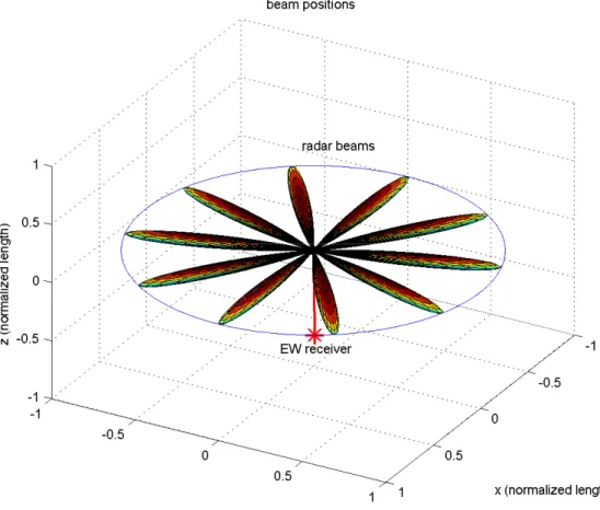
3.8 Beam positions and the EW receiver in a circular scan. . . 27
4.1 The overall flowchart of the algorithm. . . 29
4.2 An example of signal from a raster scan. . . 33
4.3 Flowchart of the preprocessing performed on the signal. . . 34
4.4 Transformed signal ready for period estimation. . . 35
4.5 Normalized autocorrelation coefficients calculated for the signal. . 36
4.6 Period estimation algorithm. . . 37
4.7 Full periods in the signal. . . 38
4.8 Final version of the signal. . . 39
4.9 Kurtosis values of the different scan patterns. . . 41
4.11 Main beams found in the signal. . . 43
4.12 Number of main beams found in the signal. . . 44
4.13 Amplitude variation of the main beams in the signal. . . 45
4.14 Time differences between the main beams in the signal. . . 46
4.15 Classification results for naive Bayes classifier. . . 48
4.16 Classification results for naive Bayes classifier with respect to dif-ferent noise levels. . . 50
4.17 The BFTree decision-tree classifier generated and used in this study. 52 4.18 Classification results for the decision tree. . . 52
4.19 Classification results for decision-tree classifier with respect to dif-ferent noise levels. . . 53
4.20 Classification results for the ANN classifier. . . 55
4.21 Classification results for the ANN classifier with respect to different noise levels. . . 56
4.22 Classification results for SVM classifier with respect to different noise levels. . . 58
Introduction
Military operations are executed in an information environment where the elec-tromagnetic spectrum is becoming increasingly more complex. Elecelec-tromagnetic devices are being used stand-alone and in networks by both civilian and military organizations and individuals for intelligence, communications, navigation, sens-ing, information storage, and processsens-ing, as well as a variety of other purposes [1]. Vulnerability in this relatively new dimension of warfare could mean a battle may be lost without even getting into contact with hostile units.
Different technological methods and military doctrines have evolved in time as the use of the electromagnetic spectrum expanded vastly in many different bands. For this very purpose, an umbrella term, Electronic Warfare (EW) is used to define any activity which has a purpose to control the spectrum, attack an enemy, or impede enemy assaults via the spectrum. The goal of electronic warfare is to deny the opponent the advantage of, and ensure friendly unimpeded access to, the electromagnetic spectrum [24]. According to the above goals, EW is divided (by US and NATO doctrines) into three main divisions: Electronic Support (ES), Electronic Attack (EA), and Electronic Protection (EP). Electronic Support’s main aim is to detect, define, recognize, and locate any electromagnetic emission particularly important for the mission. Electronic Attack, on the other hand, tries to suppress the spectrum use of the hostile units by attacking with directed electromagnetic energy or with anti-radiation missiles. Electronic protection tries
CHAPTER 1. INTRODUCTION 2
to ensure the use of the electromagnetic spectrum even in any situation where EA is employed by hostile units.
Besides these, signal intelligence (SIGINT) missions are employed on a day-by-day basis in peace time to give support to EW operations in war time. SIGINT is responsible for recording, analyzing, and forming parameter databases of the electromagnetic emissions of particular importance. SIGINT is also divided as electronic intelligence (ELINT) and communication intelligence (COMINT) in which ELINTs usually aim non-communicative emissions like radars. SIGINT is closely related to ES and in some context is the same. According to the views of the US military “the distinction between intelligence and ES is determined by who tasks or controls the intelligence assets, what they are tasked to provide, and for what purpose they are tasked” [1]. One can understand from the statement that the operations are quite similar but the purpose and the situation (combat or peace) determines the class of the mission.
This study concentrates on a problem which lies in the grounds of ES and ELINT. Its focus is an aspect of one of the most important threats in the spec-trum: radars. Radars (RAdio Detection And Ranging) are used for detection, identification and imaging of objects in the environment. For this purpose, radars emit electromagnetic energy, collect and process the reflections from these emis-sions. The radar types dealt with in this study are target detection and track radars widely used in the militaries worldwide. The RF signal that they emit has a distinct frequency (operating frequency of the radar), PRI (Pulse Repetition Interval), and PW (Pulse Width). From the return of the pulses, radars try to determine the range, speed, and the direction of the object.
Radars have several operating modes in which they perform different tasks.
Search, acquisition, and track are the fundamental modes that they deploy.
Different radars may be used for each of these purposes. As the names suggest, each mode is a step towards the final track of the target. Accurate target tracking is crucial for efficient use of weapons against the target. In these different modes, the radar beam is directed to different parts of the volume depending on the purpose. The direction of the beam can be changed electronically, mechanically
or both.
Over the years, different type of volume search methods and target tracking methods have been used in radars. These different methods, usually periodic, were all deployed in various radars of different manufacturers with different pa-rameters. These methods are mostly based on antenna scan type and antenna scan period [25].
When the other side of the picture is considered, from the EW perspective, antenna scan type and antenna scan period are vital data for use in different parts of EW systems. These parameters can be used effectively in both emitter classification and for the timing of Electronic Counter Measures (ECM) [25]. Change of scan type is also very crucial in determining the level of threat from the radar. The recognition and the estimation of period of the scan is done by EW technicians or EW officers. Despite the importance of these parameters, there is nearly no study in the open literature for automatic recognition. This is mainly because of the “classified” nature of EW studies.
The only work that is transparent related to the problem is two patents that are issued in the U.S.A [30]. The first patent, issued in 1980 describes a scan pattern generator probably finding use in EW simulators. In 2004, another patent has been issued to automatically recognize scan type, by a Lockheed Martin employee [12]. In this patent, Laplace, Fast and Discrete Fourier transforms are used. The basic scan types are determined and sample data from each type are saved in a database. The newly recorded signal is transformed to the frequency domain and correlated with the previously saved samples in the database. The type that results in the maximum correlation is stated to be the scan type of the radar. A closer look into this patent shows us that most parts of the process are left vague and the remaining transparent part is quite trivial. The change of the scan period and the variation of other parameters such as antenna beamwidth are probably assumed foreseen and looks far from robust.
Despite the scarce source of earlier work on the problem itself, some studies have been encountered in the time series data mining field from which valuable insights have been acquired. Genetic algorithms are used by Povinelli, to find
CHAPTER 1. INTRODUCTION 4
hidden temporal patterns in time series. In this study, temporary tendencies and the patterns that are possible to be observed in the future of the time series are estimated using genetic algorithms [18]. A different approach, also encountered, tries to find patterns in time series by feeding in the slopes of the series to artificial neural networks [27]. The time series is partitioned into smaller linear parts and the slopes of these smaller parts are used to extract patterns in the series. Taking Euclidean distance between the two time series to be compared may look like a trivial solution but the length of these series in time complicates the problem even if the overall pattern is the same. This problem is encountered in the speech processing field in vowel classification [11]. Vowels of each person have a shape that is quite the same but the length and the frequency of this signal varies from person to person. Dynamic Time Warping (DTW) uses linear programming to find the best possible match between different samples of the signal. If both the shape of the signal and its length changes in the same class, DTW fails to find a similarity. In our problem both the signal length (period) and its shape (because of the position of the EW receiver and radar) change in one class of data causing DTW to fail. DTW method is also used to find different patterns in series of different application areas [8, 9]. Another metric of similarity between different lengths of time series, based on state transitions of a Markov model is proposed in [28]. Similarity of time series is sometimes performed by transforming the data to another domain. The popular transforms are the Discrete Fourier Transform and Discrete Wavelet Transform [14, 19]. A comparison of these two different transforms in terms of accuracy and computational load is explored in [29].
In this thesis, an algorithm is proposed to determine both the antenna scan type and the scan period. The processed data correspond to the parameters measured in a conventional EW receiver from a particular radar. This algorithm completely automates the antenna scan analysis without the need of a human EW operator. It is also the first holistic open research output for this particular application. The proposed algorithm also provides a framework to analyze and classify periodic signals with different periodicities effectively and can be used in other fields of application as well.
about electronic warfare with emphasis on radars and their distinctive parameters. The primary focus is the antenna scan types and the scan periods. Chapter 3 explains the simulator coded to synthesize the radar signals. Chapter 4 describes the problem and gives an overview of the algorithm. It continues with the details of each step of the algorithm with the intermediate results. At the end of the chapter, validation of the algorithm with real signals and a comparison of the classifiers is presented. Chapter 5 concludes the thesis and provides some possible future research directions.
Chapter 2
Electronic Warfare Fundamentals
Radars use electromagnetic waves to be aware of the environment. Some radars are only used for target detection, some are used for tracking specific targets, some are deployed to get images of the ground. The class of radars dealt with in this study is conventional pulsed radars whose fundamental purpose is to search and track airborne targets. Continuous wave (CW) radars can also be dealt with without any problem.
Figure 2.1: A typical radar block diagram.
These radars emit electromagnetic pulses with a particular peak power. The 6
wave travels all the way to the target at the speed of light and bounces back from the target back to the radar. The received signal reflected from the target is used to determine the target’s range and direction. Some radars also estimate the Doppler velocity of the target with respect to the radar [15, 21]. The received power from a target is formulated by the well known radar equation [21]:
Pr = PtGtGrλ2σ (4πR2)2 (2.1) where Pr: received power Pt: transmitted power
Gt: transmitter antenna gain
Gr: receiver antenna gain
λ: wavelength
σ: radar cross section R: range.
Electronic Warfare (EW), on the other hand, tries to provide information about the radars in the environment and tries to jam them if possible. EW aims to protect the platform while the platform performs its mission. Detecting enemy radar pulses and classifying them are very important for the platform to be protected. The received power with an EW receiver can be found as follows:
Pr =
PtGtGrλ2
4πR2 (2.2)
If the received power is higher than the sensitivity level of the receiver, the pulse and its four main parameters are measured: frequency (F), pulse width (PW), pulse amplitude (PA), direction of arrival (DOA), and time of arrival (TOA). These parameters are measured for a CW radar by chopping up it into small pulses. The sensitivity level of the receiver depends on the bandwidth and the noise figure of the receiver. All the received pulses are classified and associ-ated with each emitter by the de-interleaving algorithms. PRI (pulse repetition interval) of the emitter is found by using the above primary parameters in the de-interleaving process [17]. Figure 2.2 illustrates these basic parameters. The distinct parameters that characterize a specific radar are F, PW, PRI, Antenna
CHAPTER 2. ELECTRONIC WARFARE FUNDAMENTALS 8
Scan Type (AST), and Antenna Scan Period (ASP). These parameters are usu-ally sufficient to determine which radar has emitted the particular pulse EW receiver has received. Another very critical piece of information is whether a radar is tracking the platform or not. This can also be inferred from AST. In the following part, the fundamental parameters that address a specific radar are ex-plained. A detailed treatment of these parameters can be found in an excellently illustrated introductory book by Stimson [22].
−2000 −1000 0 1000 2000 3000 4000 5000 6000 7000 −1.5 −1 −0.5 0 0.5 1 1.5 time (µs) pulse amplitude (V) TOA1 TOA2 PA PRI PW
Figure 2.2: Measured parameters of a typical radar pulse.
Frequency (F)
Each pulse sent by the radar is modulated with a certain frequency, the op-erating frequency of the radar. Frequency of conventional radars ranges between 1–40 GHz. Some radars also employ frequency hopping and frequency agility against jamming. F is generally used extensively in de-interleaving the pulses and emitter classification.
Pulse Width (PW)
PW is the length of the pulse in time and is usually constant for a specific radar. The range of PW is 14 µs to 1 ms. PW determines the range resolution
of the radar.
Pulse Amplitude (PA)
PA is the received power of the pulse at the EW antenna. This is directly related to the radar peak power, radar antenna gain, radar position, propagation loss (proportional to range and F), platform’s position in space and EW antenna gain.
Direction of Arrival (DOA)
Direction of arrival, as the name suggests, is the direction of the radar in the azimuth plane with respect to the platform. There are different algorithms employed in EW systems. DOA is usually found from PA ratios of different direc-tional antennas on the platform. Some EW systems also use phase interferometer systems which have comparably low errors with respect to amplitude techniques.
Pulse Repetition Interval (PRI)
PRI is the time between the pulses of the radar, sometimes called pulse repe-tition period (PRP) as well. It is found easily by differentiating TOA’s of consec-utive pulses whose emitters are the same. Radars utilize different kinds of PRI patterns. Constant, stagger, and agile PRI are the typical modes of PRI. As the name implies, in the constant PRI mode, the PRI is constant. In the stagger mode on the other hand, PRI has a deterministic pattern. In the agile mode, it has some random PRI pattern [21].
Antenna Scan Type and Period (AST-ASP)
Antennas are the crucial and indispensable part of the radar architecture. These devices are used to radiate and receive electromagnetic waves. There is a wide variety of antennas specialized for different fields of application. Radar systems use different types of antennas to accomplish their function [21].
CHAPTER 2. ELECTRONIC WARFARE FUNDAMENTALS 10
radiation pattern, directivity, gain, 3 dB beamwidth etc. Radiation pattern de-scribes the spatial distribution of the radiated power. Directivity dede-scribes how well the antenna can concentrate the input power in one direction in space. Gain takes into account the losses and inefficiencies that reduce the total radiated power from the antenna. The 3 dB beamwidth describes the angular sector where the power radiated is more than half of the maximum power radiated in the boresight direction of the antenna [6].
Antenna’s radiation pattern determines the instantaneous field of view of the radar. Typically 3 dB beamwidths, both in azimuth and elevation, of the antenna are used to calculate the visible part of the space for radar. The coverage of the antenna beamwidth is usually not sufficient for the radar’s requirements. To over-come this problem, the antenna is steered, either electronically or mechanically, to the desired part of the space [25]. Considering a hemisphere of the space to be covered, the number of steering positions can be found by the following equation:
N = 2π
∆θ∆ϕ (2.3)
where ∆θ and ∆ϕ are the azimuth and elevation beamwidths respectively. Every radar uses a different search-and-track strategy to cover the specific region it is interested in. These search strategies are called the antenna scan type (AST) of the radar. The commonly encountered ASTs are: circular, sector, raster, helical, and conical. Antenna scan period (ASP) has a very large range whose true value is usually acquired from intelligence agencies of countries. The next section describes each scan type and how it is seen from the EW receiver.
2.1
Antenna Scan Types and Their
Character-istics
As mentioned in the previous section, radars have directional antennas that direct their beams towards different parts of space as time passes. This, of course, affects directly the power received in the EW receiver. The calculation of the received
power as a function of the antenna orientation can be found as:
Pr(t) =
PtGrλ2
4πR2 Gt(θ(t), ϕ(t)) (2.4)
where Pr, Pt, Gr, λ, and R are as before and Gt(θ(t), ϕ(t)) is the transmit antenna
gain of the radar at the azimuth and elevation angles where EW receiver is located at time t.
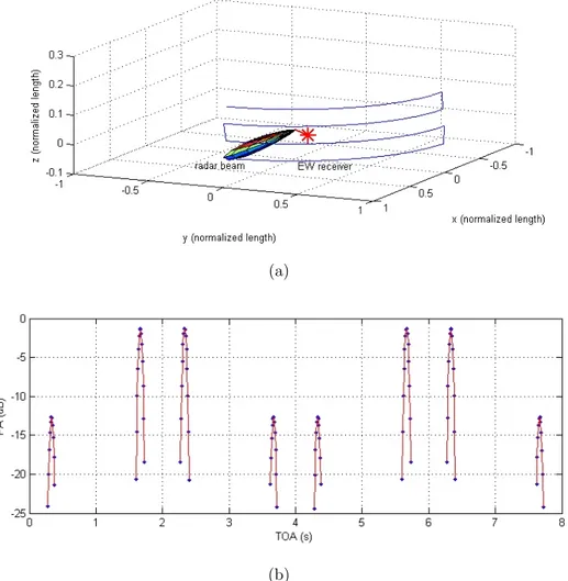
Figure 2.3 illustrates a generic antenna pattern and a respective EW receiver plotted on a unit sphere. As the antenna (beam) is turned, the EW receiver shown sees different PAs for each pulse it receives. The term PtGrλ2
4πR2 in Equation (2.4),
which is independent of time, is assumed constant because the geometry (angle and range) between the radar and the EW receiver is assumed to be changing negligibly. This assumption is valid for stationary engagement scenarios and scenarios where the antenna scan type is much faster than the system platform which is mostly the case in EW.
Figure 2.3: An example radar antenna pattern.
CHAPTER 2. ELECTRONIC WARFARE FUNDAMENTALS 12
seen that as the antenna turns to different parts of the volume, the received power changes according to the gain of the antenna at the angle where the EW receiver is located. In the following parts, ASTs mentioned above will be explained. The received power in the EW receiver will be depicted and the scan type will be introduced. The following scan types and their definitions can be found in [4] and [25].
Figure 2.4: PA received by the EW receiver as time passes.
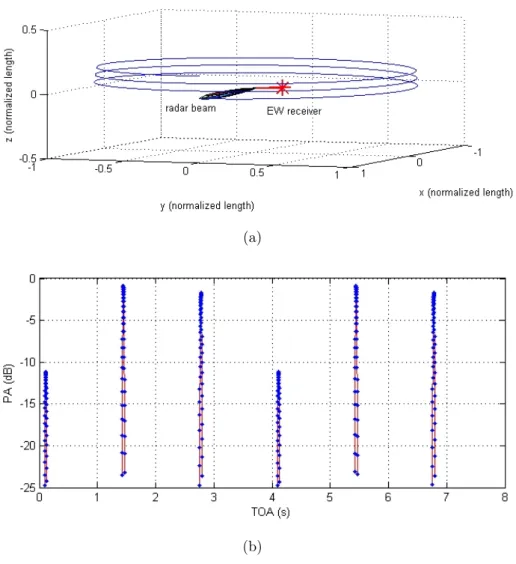
The five different signals (PA versus TOA) received by the EW receiver from the five ASTs identified in this thesis are illustrated in Figure 2.5. Each of them will be explained in detail in the following parts.
Figure 2.5: Circular, sector, helical, raster, and conical scan signals reprinted from [3].
CHAPTER 2. ELECTRONIC WARFARE FUNDAMENTALS 14
(a)
(b)
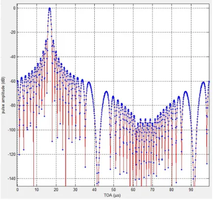
Figure 2.6: Circular scan properties: (a) the main beam positions and (b) the corresponding PA versus TOA graph.
Circular Scan: Circular scan is widely seen in search radars. The radar
con-tinues to scan the azimuth plane, 360◦ completely, with constant angular speed. The antenna has a large elevation beamwidth to see the whole elevation space. These kind of beams are called fan beams. The EW receiver effectively sam-ples the antenna pattern of the radar antenna with sampling period PRI. This is because of the fact that the pulses are received with PRI intervals in time. Figure 2.6 illustrates the main beam positions and the received PA with respect to TOA. The scan period has quite a large range in the order of 1–10 seconds.
(a)
(b)
Figure 2.7: Sector scan properties: (a) the main beam positions and (b) the corresponding PA versus TOA graph.
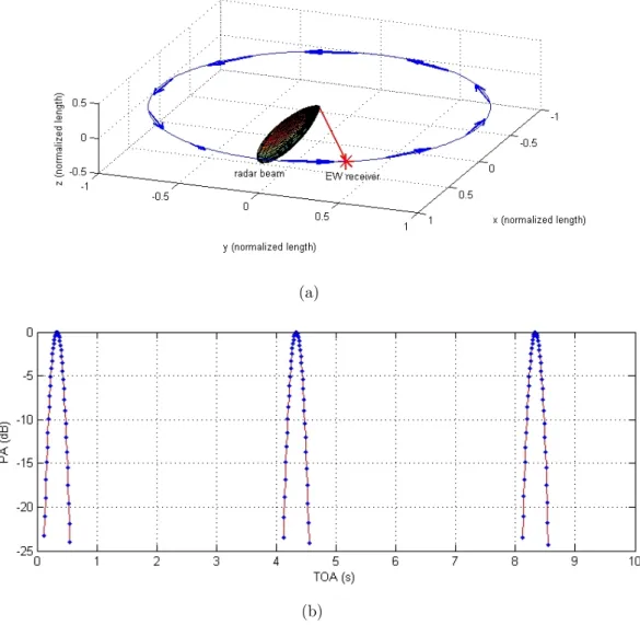
Sector Scan: Another search scan type is the sector scan. The radar scans
a specific angular sector back and forth with constant angular speed. The EW receiver receives periodic and symmetric main beams as shown in Figure 2.7(a). Figure 2.7 shows the antenna movement and the received PA time history. For each full period, two main beams are expected in this scan type. The PA received in both of the peaks are equal in magnitude. The scan period is in the order of seconds.
CHAPTER 2. ELECTRONIC WARFARE FUNDAMENTALS 16
(a)
(b)
Figure 2.8: Raster scan properties: (a) the main beam positions and (b) the corresponding PA versus TOA graph.
Raster Scan: The two scan types described above search in only azimuth,
but raster scan searches both in azimuth and elevation. The radar scans a spe-cific angular sector in azimuth and then increases its elevation after finishing the sector. It can have several bars in the elevation. The word raster comes from the fact that the movement of the beam looks like the raster scan on TV screens. The full period is constant. Since the elevation is also involved in this scan type, there is an additional loss in the PA received because of the elevation pattern of the an-tenna. Figure 2.8 shows the antenna movement and the received PA time history. In each full period, for each bar of the raster scan, a main beam is intercepted. However, the received PA changes depending on the elevation of the EW receiver.
(a)
(b)
Figure 2.9: Helical scan properties: (a) the main beam positions and (b) the corresponding PA versus TOA graph.
Helical Scan: Helical scan is also encountered in different types of radars. In
this particular scan, the radar revolves 360◦ several times like the circular scan. However, the elevation is also changed in each revolution so that the radar scans a specific sector in the elevation as well. After a complete scan period, the eleva-tion is set back to where the scan has started at the beginning. The fact that the shape of the scan resembles a helical shape is where the name comes from. The movement of the beam is shown in Figure 2.9(a). The received PA-TOA graph, shown in Figure 2.9(b), is similar to the circular scan except that the peaks of the pattern change because of the motion in the elevation plane.
CHAPTER 2. ELECTRONIC WARFARE FUNDAMENTALS 18
(a)
(b)
Figure 2.10: Conical scan properties: (a) the main beam positions and (b) the corresponding PA versus TOA graph.
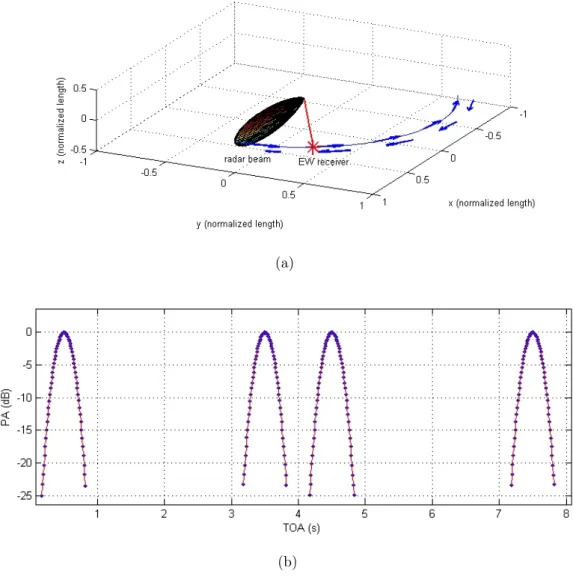
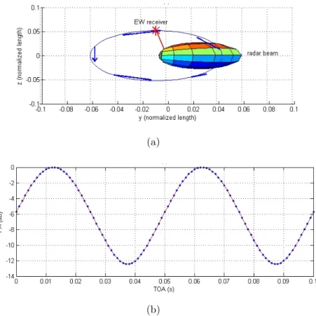
Conical Scan: This scan type is very important because it signifies that the
radar is particularly dealing with the platform EW receiver is on. It signals that the radar is trying to lock-on to the platform. The beam makes conics around the platform, trying to place the platform right on the 3 dB beamwidth. Fig-ure 2.10(a) illustrates the movement of the antenna. It first shows the start of the track process, eventually the track process converges to the perfect track in which constant PA time history is seen. The received signal, illustrated in Fig-ure 2.10(b) is like a sinusoid because of the conical action. As the lock gets better, the amplitude of the sinusoid decreases. The period of the sinusoid is distinct for every radar. Finally, when it is locked completely, that is the platform is on the 3 dB beamwidth, the received signal has a constant PA. The complete lock of this scan is sometimes called a fixed scan. The tracking process is illustrated in Figure 2.11. At the start of the track, there is an oscillation in the PA graph because of the beam getting closer and farther from the EW receiver.
0 0.05 0.1 0.15 0.2 0.25 0.3 0.35 0.4 0.45 0.5 −8 −7 −6 −5 −4 −3 −2 −1 TOA (s) PA (dB) lock on
Figure 2.11: A conical scan radar tracking the target illustrating the lock-on process.
Chapter 3
Antenna Scan Pattern Simulator
Acquiring recorded EW data is very hard if not impossible. Because of very scarce source of data, simulation of a EW receiver is performed using a MAT-LAB program. This section introduces the radar model used and the MATMAT-LAB program coded.
Figure 3.1: 3-D antenna pattern and the antenna gain at the EW receiver R [30].
Antenna Scan Pattern Simulator (ASPS) simulates the position (azimuth and elevation) of the antenna beam with respect to time. The power received from a
EW receiver is modeled according to the antenna pattern of the radar antenna and the PRI of the radar. The received power as a function of antenna orientation was given in Equation (2.4).
Figure 3.1 illustrates the antenna gain at the EW receiver. As explained be-fore, the radar antenna rotates as time passes, changing the gain seen from the EW receiver (that is the Gt(θ(t), ϕ(t)) factor in the received power) in time. The
simulator calculates the beam positions according to the scan type chosen and then determines the gain seen by the EW receiver using the receiver’s azimuthal and elevational position. The radar is assumed to be at the origin of the coordi-nate system. The received power is calculated for each pulse of the radar using its TOA and the beam’s position. The resulting PA versus TOA graph is plotted in Figure 3.2. The constant terms such as the propagation loss and EW receiver antenna gain are all assumed to be constant in the calculations. The noise level in the EW receiver is simulated by the addition of zero-mean Gaussian noise with desired power to the signal. The sensitivity level of the receiver is included in the simulations.
A Graphical User Interface (GUI), shown in Figure 3.2, is coded to ease the simulations. Each part of the GUI is explained below in detail.
3.1
TOA
This part (Figure 3.3) enables the user to input the TOAs of the pulses of radar and implicitly sets the PRI of the radar. The GUI enables three different choices for inputting the TOA. One can input directly from the edit box under the pop-up menu, from a MATLAB variable in the workspace and from a .mat file saved in the directory. The TOA values of the pulses also determine the sampling points of the antenna pattern. This part also defines the total simulation time.
CHAPTER 3. ANTENNA SCAN PATTERN SIMULATOR 22
Figure 3.2: ASPS GUI.
Figure 3.3: TOA input part of the GUI.
3.2
EW Receiver Properties
This part (Figure 3.4) inputs the EW receiver properties and receiver position with respect to the radar. The azimuth and the elevational position of the receiver is given in degrees. It is assumed that the EW receiver is stationary (or moves by a negligible amount compared to the radar) throughout the simulation time. The noise and the sensitivity level of the receiver can be configured as well. Gaussian noise with desired power is added to the signal level. Signals with amplitude below the sensitivity level of the receiver will be ignored because it is quite likely
that they are noise. This comes from the detection mechanism of the EW receiver.
Figure 3.4: EW receiver position with respect to the radar.
3.3
Antenna Model
The antenna model and its beamwidth are configured in this part (Figure 3.5) of the GUI. Six different antenna models are implemented in the simulator: uniform, triangle, Hamming, Taylor, Poussin, and Blackman. The side lobe levels of the antenna patterns differ in each case. The user also inputs the beamwidths in azimuth and elevation. The simulator calculates the number of elements needed to achieve the input beamwidth for the particular model. After this calculation, simulator synthesizes a pattern for azimuth and elevation. According to the receiver’s position, it calculates the pattern gains in azimuth and elevation and multiplies them with each other to find the overall pattern at the particular azimuth and elevation. The different parameters needed for each model can be input as well by changing the pop-up menu.
CHAPTER 3. ANTENNA SCAN PATTERN SIMULATOR 24
Figure 3.5: Antenna model and beamwidth configuration panel.
3.4
Antenna Scan Type Properties
This part (Figure 3.6) of the GUI lets the user choose the AST properties. The scan type of the radar is selected first. According to the scan type, different edit boxes are enabled with respective parameter names. The user inputs the parameters for the particular scan type. Circular, sector, raster, helical, and conical scans are simulated by the environment. Period is the common parameter for all of the scan types. Sector scan needs the start-finish positions in the azimuth and the elevation position of the beam. Raster scan acquires the start-finish positions in azimuth and elevation with the number of bars in the elevation. Conical scan type needs the target azimuth and elevation position and squint angle of the radar. All of the above parameters are used to calculate the beam position at a specific point in time which is basically the TOA of the pulse. The pulse with the maximum power is normalized to 0 dB.
3.5
Antenna Scan Pattern Plot
The axes in these parts (Figure 3.7) are used to plot PA versus TOA of the simulated scenario. The zoom, pan, and rotate buttons of the figure can be used to explore the signal further.
Figure 3.6: Antenna scan properties configuration panel.
3.6
Beam Positions
The simulator also illustrates how the beam scans the volume as time passes. It divides the whole simulation time into 10 intervals. It illustrates the beam position at these time points and also plots the position of the EW receiver to see the effects of the rotation of the beam. An example of a circular scan is given in Figure 3.8, where the beams and the EW receiver position are illustrated.
CHAPTER 3. ANTENNA SCAN PATTERN SIMULATOR 26
Chapter 4
Antenna Scan Type Recognition
Algorithm
Antenna scan analysis problem can be ideally formulated as finding the angles between the radar main beam and the EW receiver as time passes and then trying to classify the radar scan pattern into one of the most encountered scan types. This information is supposed to be inferred from the power received from the radar. However, the problem is complicated in various ways: the radiation pattern and the location of the radar antenna are completely unknown to the EW system, and the parameters of the scan types vary vastly (antenna scan period, number of bars in raster, sector width etc.) which is almost always the case in the practical world. Trying to check all the possible received power outcomes and defining a metric (e.g., Euclidean distance) to measure the similarity would exhaust any computation power feasible. The deficiency of vital information has lead the study to suboptimal solutions in which the main phenomena for recognition, period and main beam positions and numbers, are used.
This chapter starts with an overview of the algorithm. It is first presented as a general algorithm because the proposed algorithm framework can be used in other applications such as vowel classification in speech recognition as well. Following the main framework, application of the algorithm to the specific problem of radar
antenna scan analysis is explained with a running example. The parameters of the general algorithm are also tuned to the signals of interest in Section 4.2. The results of the intermediate parts are also given as the algorithm is explained. The algorithm is validated by both synthetic data generated by ASPS and real data acquired and provided by ASELSAN Inc.
4.1
Overview of the Algorithm
This section explains the proposed algorithm step by step with general inputs and outputs suitable for the classification of any periodic signal. The algorithm can be used, not only for the particular problem of this thesis, but also to classify uniformly or non-uniformly sampled periodic signals. The parameters such as the thresholds or the value of N should chosen according to the specific signals involved.
CHAPTER 4. ANTENNA SCAN TYPE RECOGNITION ALGORITHM 30
4.1.1
The Input Signal
We assume that the input signal x[l] is a discrete-time sequence obtained by properly sampling the original signal x(t) above the Nyquist rate. The sampling procedure is as follows:
x[l] = x(lTs) l = 0, 1, . . . , L− 1 (4.1)
Although uniform sampling is employed in many applications, in some cases, non-uniformly sampled signals can be encountered as well. Uniformly sampled signals are much simpler to handle. Calculating the period of a uniformly sampled signal is easier and less complex, usually independent from the method used. If one has a non-uniformly sampled signal, it is better to resample the signal with a sampling rate suitable to the signal so that it becomes uniformly sampled. Different interpolation (linear, polynomial etc.) techniques can be applied for resampling.
4.1.2
Period Estimation
A signal x[l] is considered periodic if a period value T exists such that
x[l] = x[l + mT ] ∀l, m. (4.2) The smallest value of T that satisfies this equation is called the fundamental period. Period estimation has attracted a lot of interest over the years especially in the speech processing area [5, 10, 16, 31]. The problem is sometimes called (fundamental) tone estimation or pitch estimation as well. There are solutions to the problem in the time and the frequency domains.
Frequency-domain methods use the fundamental idea behind the Fourier transform. The period is estimated by looking at the peaks of the frequency content. This method works well for sinusoids, since it was designed for this purpose, but it possesses some problems when the signal is not a sinusoid. For example, if the spectrum of the signal itself is broad, the peaks may be illusive when estimating the fundamental frequency.
Time-domain methods are particularly useful for period estimation of non-sinusoidal signals. These methods define some kind of similarity metric, and by this metric, try to maximize the similarity with the lagged versions of the signal. The lag where the similarity is maximized becomes the period of the signal which is quite intuitive. Absolute magnitude difference function (AMDF) uses the difference of the signal and lagged versions of the signal as a metric [31]. Autocorrelation function is also employed in which the correlation between the signal and its lagged versions are used as a similarity metric. There are modified versions of these techniques to enhance the results of period estimation [31].
The backbone of our algorithm is the period estimation part. This part affects the overall performance of AST classification significantly. The period estimation method should be chosen suitably, according to the properties of the signal.
4.1.3
Normalize, Resample, and Average
This part mainly describes the preprocessing stage before the features are ex-tracted. It tries to minimize the noise and transform the signal into standard dimensions, eventually improving the quality of the features.
The signal can be normalized so that the features are not affected by the range of the signal. The most suitable normalization technique should be chosen among the different normalization techniques (e.g., range normalization, standard deviation normalization) according to the signal properties.
The input signal could be from a set where the sampling rates and the number of samples could be widely varying, which is the case in our application. To extract reasonable features from this type of signal, it is better to have the same number of samples and the sampling rate should be somewhat similar. This improves the quality of the features and reduces their dependency on the length of the signal and the sampling rate.
The number of samples (N ) that define the signal sufficiently well is deter-mined by analyzing the signal. The sampling interval of the original discrete-time
CHAPTER 4. ANTENNA SCAN TYPE RECOGNITION ALGORITHM 32
signal with total length L is changed from Tsto NT after the resampling procedure
by: xr[k] = x[round( kTs T N )] k = 0, 1, . . . ,⌊ (L− 1)T TsN ⌋ (4.3)
where xr[k] denotes the resampled sequence and ⌊.⌋ indicates truncation. The
procedure above uses nearest point interpolation for non-integer NT
Ts values. One
can also use sinc, linear, or spline interpolation.
If the signal has at least two periods, it can be coherently added and averaged so that the effect of noise is reduced. Assuming the signal has at least M (L≥
M N ) full cycles, the averaging process for the resampled signal is performed as
follows: x[k] = 1 M M∑−1 m=0 xr[k + mN ] k = 0, 1, . . . , N − 1 (4.4)
4.1.4
Feature Extraction
After the signal has been transformed into N sampled points with the preceding procedures, it is ready for the feature extraction stage. Different features of the signal such as the minimum and the maximum values, mean, standard devia-tion, skewness, kurtosis or higher-order moments are usually used to describe the probability density function of the signal. The features to be extracted change from signal to signal according to the phenomena that affect the classes. Coeffi-cients of the Fast Fourier Transform (FFT), Discrete Cosine Transform (DCT), and Discrete Wavelet Transform (DWT) are used extensively in the literature [14, 19, 29].
4.1.5
Classification
The classification phase is the intelligence part of the whole system. There is a wide variety of classifiers, to name a few [7]: Bayesian classifier, Gaussian discriminants, artificial neural networks, decision trees, support vector machines etc.
4.2
Application of the Algorithm to Radar
An-tenna Scan Analysis Problem
4.2.1
The Input Signal
The signal consists of a discrete-time sequence of PAs versus TOAs of the pulses which are either the output of the ASPS or collected via the EW receiver. Fig-ure 4.2 shows an example PA versus TOA signal. The output from these sources
Figure 4.2: An example of signal from a raster scan.
are in dBW (decibel relative to watt). The signal is first transformed from dBW to Volt (V) scale by:
voltage = 10(power/20) (4.5) It is assumed that the input signal has at least two cycles of the antenna scan. This is important since period estimation phase needs at least a few cycles to accurately estimate the period of the signal. The input signal has a variety of dif-ferent parameters. The PRI, ASP, azimuth and elevation beamwidth parameters of the radar and the receiver are changed at every signal synthesized so that the classifiers encounter all the different variety of parameters that affect the signal. Parameter selection of synthesized signals is made realistically taking real radar systems as examples.
CHAPTER 4. ANTENNA SCAN TYPE RECOGNITION ALGORITHM 34
Some of the signals are assumed to have stagger type PRI which means that the sampling rate is not uniform. As already stated in the previous chapter, work-ing with uniformly sampled signals is much simpler and has less computational complexity. If the signal has stagger PRI, it is resampled in this part with the highest PRI in the stagger levels. During the resampling process, if the signal is not available at a particular time point, interpolation is performed using the two closest points. In some cases, especially when the antenna is looking towards the opposite of the EW receiver, the receiver does not sense any pulses. These points are filled with zeros to make the succeeding computations easier. The flowchart of this part is shown in Figure 4.3. As a result, the signal in Figure 4.2 is transformed into the signal shown in Figure 4.4.
CHAPTER 4. ANTENNA SCAN TYPE RECOGNITION ALGORITHM 36
4.2.2
Period Estimation
The period estimation is based on the normalized autocorrelation coefficients of the signal, defined as follows:
rxx[k] = ∑W−1 i=0 x[i]x[i + k] √∑W−1 i=0 x2[i] √∑W−1 i=0 x2[i + k] k = 0, 1, . . . , L− W (4.6)
W in Equation (4.6) is the window size that should be chosen such that a
com-promise between computational complexity and accuracy is reached. In the algo-rithm, it has been chosen as one third of the signal length (W = L3). An example of rxx[k] is shown in Figure 4.5. The threshold level of 0.98 is also drawn on the
figure in dashed lines.
0 500 1000 1500 2000 2500 3000 3500 4000 4500 5000 0 0.1 0.2 0.3 0.4 0.5 0.6 0.7 0.8 0.9 1 k,lags rxx rxx threshold
Figure 4.5: Normalized autocorrelation coefficients calculated for the signal.
After calculating the correlation coefficients between the signal and its lagged versions, the algorithm outlined in Figure 4.6 is employed to estimate the final period. Applying the algorithm in Figure 4.6 to Figure 4.5, one can see that the period is 2500 lags.
CHAPTER 4. ANTENNA SCAN TYPE RECOGNITION ALGORITHM 38
4.2.3
Normalize, Resample, and Average
This part prepares the signal for the feature extraction phase by normalizing, averaging, and finally resampling the signal.
The normalization process is quite simple where the signal is simply scaled by its maximum value so that the signal varies between 0 and 1:
xnorm[k] =
x[k]
max(x[k]) k = 0, 1, . . . , L− 1 (4.7) This process tries to remove the effects of propagation, since propagation results in a decay in pulse amplitude, proportionate to the distance between the radar and the EW receiver. Here, we are not concerned with the distance and rather concerned with the antenna scan type which is independent of constant decays.
Figure 4.7: Full periods in the signal.
Next, we resample the signal so that the total number of samples from one cycle of a particular scan type is N where the value of N depends on the signal. This process transforms all of the recorded signals from different radars with different PRIs, different ASTs and different ASPs with T
signal vector with N elements. Here, T is the estimated period and Ts is the
sampling interval of the original signal. The process also regularizes the different sampling periods of the signal to NT. The value of N is chosen as 2000 throughout the example signal. This resampling phase also reduces the amount of data because radars use much larger number of pulses per scan period to be aware of the environment, so it becomes a decimation operation. Since a high sampling rate is available before the resampling phase, nearest point interpolation technique can be used with negligible distortion in the signal. This process was defined in Equation (4.3).
Assuming M full cycles of signal are available to estimate the period of the signal, the signal can coherently be averaged using Equation (4.4) to decrease the effect of noise. Figure 4.7 shows the signal with the periodic parts shown in green boundaries. The final version of the signal is pictured in Figure 4.8. From this point on in the text, the word “signal” is used for the final version of the signal.
0 200 400 600 800 1000 1200 1400 1600 1800 2000 0 0.1 0.2 0.3 0.4 0.5 0.6 0.7 0.8 0.9 1 sample number
normalized and averaged PA (mV)
CHAPTER 4. ANTENNA SCAN TYPE RECOGNITION ALGORITHM 40
4.2.4
Feature Extraction
In this section, we describe the four features selected and used by the algorithm. Input to this part is the preprocessed N element signal with sampling interval NT. There are a total of 100 data points, 20 from each of the following scan types in the following order: circular, sector, raster, helical, and conical. These signals are synthesized by using the ASPS described in the previous chapter. The parameters (azimuth and elevation beamwidths, sector width, number of bars in raster, scan period etc.) used while generating the signals are very important. The results of the classification phase could be very misleading if the parameters are not set appropriate with the real world examples. Therefore, we have used a classified database which the parameters of the radars are accountable on and have selected these parameters accordingly.
We have attempted to use a number of different features such as the mean, standard deviation, and skewness, but the best results were obtained with the four features described below:
Kurtosis of the Signal
Kurtosis is the normalized fourth-moment of a random variable X and is defined as:
kurtosis = E[X− µ]
4
σ4 (4.8)
where µ is the mean and σ is the standard deviation of the random variable. Kurtosis is a statistical measure of how peaked or how flat the distribution of the random variable is. It can also be seen as a measure of how heavy the tails of the distribution are relative to the Gaussian distribution which has a kurtosis value of 3. Concentrated distributions such as the uniform distribution have kurtosis values less than 3. If the distribution has heavier tails and is more outlier prone, its kurtosis value exceeds 3.
In track modes, radars try to illuminate the threat as much as possible so that they can update the threat’s coordinates finely and accurately for a possible
attack. To perform this task, they have to steer the beam such that it is on the platform all of the time. This in turn means that the EW receiver will get all the pulses of the radar with slight differences in amplitude (i.e., a narrow distribution of amplitude) depending on the track scanning type of the radar system. The amplitude variation is approximately uniform. A conical scan signal, which is a uniformly sampled sinusoid, has a kurtosis value of around 1.5. By looking at the signal’s kurtosis value, the system will get an idea about its mode and scan. The kurtosis value will be small for conical scan and large otherwise. This fact is confirmed by Figure 4.9 which illustrates that for the conical scan, kurtosis of the signal can be used as a discriminator. Therefore, we select the kurtosis as the first feature: F1 = kurtosis(x[k]) (4.9) 0 10 20 30 40 50 60 70 80 90 100 0 50 100 150 200 250 300 350 400
data point number
kurtosis
circular sectoral raster helical conical
Figure 4.9: Kurtosis values of the different scan patterns.
Cross Correlation of the Signal with the Main Beam
It can be observed by analyzing different scan types and their effect on the EW platform that the position of the main beam differentiates the scans from each other. The phenomenon behind the data reveals this information very clearly. The radar is trying to search different volumes of space with different periodic
CHAPTER 4. ANTENNA SCAN TYPE RECOGNITION ALGORITHM 42
strategies. So the relation of the time between the main beams and the amplitude variation of the main beams are the key parameters for a robust recognition system.
First, the algorithm has to detect the main beam in the signal. This can be achieved quite easily by finding the maximum point in the signal. Assuming that there is a main beam in the signal, this has to be the maximum point. From the index of the maximum point, it starts to advance indices until the magnitude drops to 0.01. The process is repeated exactly in the same way for the pulses previous to the maximum point. By using these two points neighboring the maxi-mum point where the amplitude drops to 0.01, it extracts the main beam between these two points. Figure 4.10 illustrates the signal and the main beam detected in the signal. After finding one of the main beams in the signal, the algorithm
0 200 400 600 800 1000 1200 1400 1600 1800 2000 0 0.1 0.2 0.3 0.4 0.5 0.6 0.7 0.8 0.9 1 sample number
normalized and averaged PA (mV)
pulse amplitudes pulse amplitudes main beam
Figure 4.10: Main beam found in the signal.
detects all of the possible main beams in the signal by using the normalized cross correlation between the signal and the main beam found. The normalized cross correlation between two discrete sequences x[n] and y[n] is defined as follows:
rxy[k] = ∑V−1 i=0 x[i]y[i + k] √∑V−1 i=0 x2[i] √∑V−1 i=0 y2[i + k] (4.10)
in this study) and finding the peaks in the cross correlation values gives all the possible main beams.
0 200 400 600 800 1000 1200 1400 1600 1800 2000 0 0.1 0.2 0.3 0.4 0.5 0.6 0.7 0.8 0.9 1 sample number
normalized and averaged PA (mV)
pulse amplitudes main beams
Figure 4.11: Main beams found in the signal.
One would expect the cross correlation value to be large since the patterns of different antennas are very similar near their bore sights. For scan types where no elevational action is involved (circular and sector), the main beams will be exactly the same, ignoring the effect of noise. The threshold can be tuned according to the signal to be able to handle the possible variations in the azimuth pattern caused by the changing elevation angle. Figure 4.11 shows the main beams found in the signal.
After finding the possible main beams in the signal, some very important relations are calculated from the time position and the pulse amplitudes of the main beams.
The number of main beams is an important parameter that can differentiate some scan types from the others. In particular, the circular scan has only one beam in one period which is a valuable feature to discriminate it from the others. Figure 4.12 shows this feature for all the data points. The figure shows that this feature is indeed very useful for classification. Circular and sector scan types are
CHAPTER 4. ANTENNA SCAN TYPE RECOGNITION ALGORITHM 44
very visible in the figure by this parameter. It can also be seen that no main beam is found in the conical signal since the pulse variation is not observed. Therefore, we choose the second feature as the number of main beams:
F2 = number of main beams in the signal (4.11)
0 10 20 30 40 50 60 70 80 90 100 0 1 2 3 4 5 6 7 8 9
data point number
number of main beams
circular sectoral raster helical conical
Figure 4.12: Number of main beams found in the signal.
Amplitude variation of the main beams can also be a very useful feature. The range of the main beam amplitudes is used as a measure of the variation by subtracting the minimum amplitude from the maximum amplitude. This feature can differentiate between azimuthal and elevational scan types. More generally, this feature can differentiate the scan types that involve only one plane (azimuth) and the ones that scan both planes (azimuth and elevation). Therefore, the third feature becomes the amplitude variation of the main beams:
F3 = max(main beam PAs)− min(main beam PAs) (4.12)
Figure 4.13 shows the distribution of this feature for all data points. One can see that the variation could not be calculated for circular scan types since this
0 10 20 30 40 50 60 70 80 90 100 0
0.5 1 1.5
data point number
amplitude variation of main beams
circular sectoral raster helical conical
Figure 4.13: Amplitude variation of the main beams in the signal.
type of scan produce only one main beam. Similarly, since the conical scan does not have any distinct main beam, variation of main beams is not calculated as well. However, it is observed that the sector scan type can be separated from the others with this feature.
Time difference between the main beams is also a distinctive parameter be-tween classes. Circular and helical scan types revolve the 360◦ sector continuously without going back and forth like sector and raster scans. In this case, one ex-pects to see the time difference between the main beams to be very similar. However, in the raster scan, the time difference between the main beams should vary most of the time because of the nature of the scan. The only case where the time difference will be the same is when the EW receiver is in the middle of the scanned sector which is unlikely. For this, max(time differences)min(time differences) is calculated and used as a parameter. This parameter is plotted for all the different data points in Figure 4.14. We observe that this feature is only calculable for helical and raster scans since there should be at least three main beams to calculate the variation of time differences between the main beams. Therefore, the final feature is chosen
CHAPTER 4. ANTENNA SCAN TYPE RECOGNITION ALGORITHM 46
as the variation of the time differences:
F4 = max(time differences) min(time differences) (4.13) 0 10 20 30 40 50 60 70 80 90 100 0 1 2 3 4 5 6 7 8 9
data point number
variation of time differences
circular sectoral raster helical conical
4.2.5
Classification
The above features are used in the classification phase. For features that cannot be calculated for different scan types, 10000 value is used as a numeric value for the classification algorithm input as an indicator. For example, a main beam cannot be observed in a conical scan so its features other than the kurtosis cannot be calculated and set as 10000 to ease the calculations in the classification part. Four different classification techniques are used: naive Bayes, decision tree, multilayer perceptron neural network, and support vector machines. The clas-sification rates according the N parameter of the algorithm is shown to see the effect of the number of samples per period. The classification methods and their results are presented below. An open source machine learning software WEKA, developed by The University of Waikato, is used in the classification process [23]. We have used 4-fold cross-validation technique for training and testing the algorithm. In this cross-validation technique, the data points from each class are randomly partitioned into four groups. In the first run, first part is retained for testing and the remaining is used for training. In the second fold, the second part is retained for testing and the remaining is used for training. All of the data points are tested by this procedure by repeating this procedure four times [26].
4.2.5.1 Naive Bayes
Naive Bayes classifier classifies according to the Bayes’ theorem. The classifier calculates the posterior probabilities according to the models of each class. The decision rule for classification is merely picking the hypothesis that is more prob-able.
Assuming w1, w2, . . . , wn are the classes, p(x|wj) is the state-conditional
den-sity function assuming that the given class is wj, then the posterior probability
is calculated as follows:
p(wj|x) =
p(x|wj)p(wj)
CHAPTER 4. ANTENNA SCAN TYPE RECOGNITION ALGORITHM 48
where p(x) =∑nj=1p(x|wj)p(wj) is the total probability.
In the training phase, probability models for p(x|wj) are calculated using the
training signal for each wj. The probability density function is assumed to be
a normal distribution and the parameters of the distribution are calculated by maximum likelihood estimation. In naive Bayes method, each of the features are assumed independent and the calculations of the parameters of the model are made accordingly. This assumption greatly simplifies the calculations and the complexity of the model.
The classification phase calculates the posterior probabilities according to Equation (4.14). The class of the signal is chosen as the most probable class according to the calculated posterior probabilities [7].
Figure 4.15 shows the classification results with respect to different N values. It can be seen that for very small N , the signal is undersampled and the features are not correctly extracted, causing errors in the classification. One can conclude from the figure that N = 1000 is a good choice in terms of the correct classification rate and computational complexity.
0 500 1000 1500 2000 2500 3000 3500 4000 70 75 80 85 90 95 100
N (number of samples per period)
correct classification percentage
Figure 4.15: Classification results for naive Bayes classifier.
A confusion matrix in the case of N = 1000 is shown in Table 4.1.
classification result
circular sector raster helical conical
true class circular 19 1 0 0 0 sector 1 19 0 0 0 raster 0 0 20 0 0 helical 0 0 0 20 0 conical 0 0 0 0 20
Table 4.1: Confusion matrix for naive Bayes classifier with 98% correct classifi-cation rate.
noise affects the detected signal levels because of the thresholding in the detection phase of the pulses. A threshold level of 10 dB above the noise power level is used in this analysis. This threshold value is usually used in EW systems as a good compromise between probability of false alarm and probability of detection [25]. The thresholding limits the range of the PA versus TOA signal. This, of course, may result in the loss of main lobes especially in raster and helical scans, leading to classification errors. For example, because of the limited range of the signal, only one bar of the raster scan may be observed leading to a circular scan classification erroneously. The classification result with respect to the SNR is shown in Figure 4.16 where we used SNR values of 12, 15, 20, 25, 30, 35, and 40 dB. The breakdown in the performance around 25 dB SNR shows us the effects discussed earlier because of the range of the signal. The confusion matrix in Table 4.2 shows the effect more clearly. The limited range of the signal indicates a tendency towards sector and circular scan both of which are only azimuthal scans and are relatively immune to the range of the signal received. We have also observed that when the sinusoidal shape in a conical scan is distorted by loss of pulses, the algorithm also has a tendency towards circular scan.
CHAPTER 4. ANTENNA SCAN TYPE RECOGNITION ALGORITHM 50 10 15 20 25 30 35 40 20 30 40 50 60 70 80 90 100 SNR (dB)
correct classification percentage
Figure 4.16: Classification results for naive Bayes classifier with respect to differ-ent noise levels.
classification result
circular sector raster helical conical
true class circular 19 1 0 0 0 sector 1 19 0 0 0 raster 6 0 4 10 0 helical 0 5 0 15 0 conical 2 0 0 0 18
Table 4.2: Confusion matrix for naive Bayes classifier in the case of 20 dB SNR (77% correct classification).
![Figure 2.5: Circular, sector, helical, raster, and conical scan signals reprinted from [3].](https://thumb-eu.123doks.com/thumbv2/9libnet/5607975.110704/26.892.174.774.235.968/figure-circular-sector-helical-raster-conical-signals-reprinted.webp)
![Figure 3.1: 3-D antenna pattern and the antenna gain at the EW receiver R [30].](https://thumb-eu.123doks.com/thumbv2/9libnet/5607975.110704/33.892.315.651.673.975/figure-d-antenna-pattern-antenna-gain-ew-receiver.webp)