Research Article
Modeling Traders’ Behavior with Deep Learning and Machine
Learning Methods: Evidence from BIST 100 Index
Afan Hasan ,
1Oya Kalıpsız ,
2and Selim Akyokus¸
3 1Sabanci School of Management, Sabanci University, Istanbul, Turkey2Computer Engineering Department, Yildiz Technical University, Istanbul, Turkey 3Computer Engineering Department, Istanbul Medipol University, Istanbul, Turkey Correspondence should be addressed to Afan Hasan; [email protected]
Received 23 December 2019; Revised 15 April 2020; Accepted 27 May 2020; Published 29 June 2020 Academic Editor: Eulalia Mart´ınez
Copyright © 2020 Afan Hasan et al. This is an open access article distributed under the Creative Commons Attribution License, which permits unrestricted use, distribution, and reproduction in any medium, provided the original work is properly cited. Although the vast majority of fundamental analysts believe that technical analysts’ estimates and technical indicators used in these analyses are unresponsive, recent research has revealed that both professionals and individual traders are using technical in-dicators. A correct estimate of the direction of the financial market is a very challenging activity, primarily due to the nonlinear nature of the financial time series. Deep learning and machine learning methods on the other hand have achieved very successful results in many different areas where human beings are challenged. In this study, technical indicators were integrated into the methods of deep learning and machine learning, and the behavior of the traders was modeled in order to increase the accuracy of forecasting of the financial market direction. A set of technical indicators has been examined based on their application in technical analysis as input features to predict the oncoming (one-period-ahead) direction of Istanbul Stock Exchange (BIST100) national index. To predict the direction of the index, Deep Neural Network (DNN), Support Vector Machine (SVM), Random Forest (RF), and Logistic Regression (LR) classification techniques are used. The performance of these models is evaluated on the basis of various performance metrics such as confusion matrix, compound return, and max drawdown.
1. Introduction
The efficiency of technical analysis, one of the oldest in-struments used to predict market direction, has long been debated, and the discussion seems likely to continue. The main reason for this is that, to predict future market trends, the technical analysis is likely to use information such as past price and past volume, which is not based on fundamental analysis. This violates the classical market efficiency theory [1].
Investors are thought to be one of the most important drivers of volatility in stock prices as a result of repetitive
patterned trading behavior. This leads to the idea that stock
prices are following the trends that form the basis of technical analysis [2]. Although patterned trading behavior does not seem logical to some, it is known that investors are using it to predict market trends and predict future price movements effectively.
The basic information that technical analysts use is
volume and price. In technical analysis studies, the patterns
in the historical stock exchange series arising from daily market activities are examined in order to predict future market movements.
Despite ongoing debate on the effectiveness of technical analysis, the emergence of traders applying technical analysis in practice may be even more motivating to carry out new studies in this area [3–7]. For example, a survey conducted on 692 fund managers indicates that 87% of them pay at-tention to technical analysis while making investment de-cisions [8].
In financial trading, technical and quantitative analysis uses mathematical and statistical tools to determine the most appropriate time for investors to initiate and close their orders, which means instructions for buying or selling on a trading venue. While these traditional approaches serve to some extent their purpose, new techniques emerging in
Volume 2020, Article ID 8285149, 16 pages https://doi.org/10.1155/2020/8285149
computational intelligence such as machine learning and data mining have also been used to analyze financial information.
One of the main objectives of machine learning methods is to find hidden patterns in the data by using automatic or semiautomatic methods. Useful patterns allow us to make meaningful estimates on new data [9]. Machine learning techniques used in real life, such as time series analysis [10], communication [11], Internet traffic analysis [12], medical imaging [13], astronomy [14], document analysis [15], and biology [16], have demonstrated impressive performance in solving classification problems. While the vast majority of previous financial engineering research focuses on complex computational models such as Neural Networks [17–20] and Support Vector Machines [21, 22], there is also research based on new deep learning models that yield better results in nonfinancial applications [23, 24].
Deep learning is one of the machine learning methods that use past data to train models and make predictions from new data. Recent developments in deep learning have allowed computers to recognize and tag images, recognize and translate speech, be very successful in games that require skill, and even perform better than human beings [25]. In these applications, the goal is usually to train a computer to perform tasks that humans can do as well. Deep learning methods allow the task to be performed without human participation; perhaps the task that can be done differently by a person is unlikely to be completed with human power over a limited period of time, or there is too much of a benefit in tasks where supernatural performance is needed, as in the case of medical diagnoses [26].
Current state-of-the-art practices of deep learning differ from market direction forecasting problems in many as-pects. However, one of the most striking aspects is that market forecasting problems are not those that people can already do well. Unlike interpreting, perceiving objects in a picture, understanding texts in the pictures, people do not have the innate ability to choose a stock that will perform well in some future periods. However, deep learning tech-niques may be useful for such selection problems because these techniques essentially convert any function mapping data to a return value. At least, in theory, a deep learner can find a return value for a relationship among data, no matter how complex and nonlinear it is. This is far from both the simple linear factor models of traditional financial eco-nomics and relatively coarse statistical arbitrage methods, and other quantitative asset management techniques [27].
In this study, we investigate the benefits of Deep Neural Network (DNN), Support Vector Machine (SVM), Random Forest (RF), and Logistic Regression (LR) classifiers in making decisions on market direction. In particular, we show whether these classification approaches can make trading consistent and profitable for a long period of time. The main contribution of the study is developing a deep learning model taking into consideration OHLC prices and transaction costs and also to compare the classification performance of the developed model with the most com-monly used machine learning methods on estimating the direction of a stock market index. The success of deep
learning and machine learning methods may differ according to the inefficiencies of the markets [28]. This study investigates the case of Stock Exchange Istanbul and emerging markets. Another contribution of this study is the use of threshold values to control transaction costs in fi-nancial estimates. In some studies, transaction costs are not covered, although estimates seem profitable. It is known that when transaction costs are included, profitability may dis-appear [23]. To avoid this problem, the threshold level is dynamically adjusted according to the standard deviation of the profit distribution, and optimal values are selected to reduce the number of transactions in order to increase the return (profit on an investment) per transaction. Accord-ingly, the aim is to create profitable operations in the long run with the right combination of parameter values and property selection of the training set size.
The structure of the paper is organized as follows. Section 2 provides the related work and similar studies of deep learning and machine learning in making decisions on market direction. Section 3 briefly describes the method-ology, general experimental setup, datasets, the attribute selection for feeding the models, the specific parameter settings to provide comprehensive information for deep learning, and other machine learning algorithms used in experiments and their use in future work. The results of the analysis of each of the trading scenarios are presented in Section 4. Finally, Section 5 concludes the study by providing the obtained results and future considerations.
2. Related Work
Researchers have intensified their studies on the direction of movements of various financial instruments using time series and machine learning methodologies. Both academic researchers and practitioners have developed financial trading strategies to make forecasts about future movements of the stock market index and transform the predictions into profits. This section includes a summary of research about the stock prediction that covers methods that use technical indicators as features, traditional machine learning algo-rithms, studies done for Istanbul Stock Exchange (ISE), and current methods that use deep learning algorithms in finance.
The majority of the studies based on stock market prediction with machine learning algorithms use technical indicators as part of the training dataset. Neural Networks (NN) [17, 18] and Support Vector Machines (SVM) are one of the mostly used machine learning methods. There are also studies that use classification methods such as Decision Trees (DTs) [29], Random Forests (RFs) [30], Logistic Re-gression (LR) [31], and Naive-Bayes (NB) [32]. Patel et al. [33] focused on predicting future values of Indian stock market indices using Support Vector Regression (SVR), Artificial Neural Network (ANN), and Random Forest (RF). The best overall prediction performance is achieved by SVR-ANN hybrid model. Accuracy in the range of 85–95% has been achieved for long-term prediction on stocks such as AAPL, MSFT, and Samsung using Random Forest classifier by building a predictive model in Khaidem’s research [34].
Buy, hold, or sell decision prediction is performed on Stock Exchange of Thailand (SET) by Boonpeng and Jeatrakul [35], comparing the performance of the traditional neural network with One vs. All (OAA) and One vs. One (OAO) neural network (NN). With an average accuracy of 72.50%, OAA-NN showed better output than OAO-NN and tradi-tional NN models.
In order to improve the profitability and stability of trading that includes seasonality events, Booth et al. [36] introduced an automated trading system based on perfor-mance weighted ensembles of random forests. Tests are done on a large sample of stocks from the DAX, and they have found that recency-weighted ensembles of random forests produce superior results. The research in [37] investigated methods for predicting the direction of movement of stock and stock price index for Indian stock markets, by com-paring four machine learning prediction models: Artificial Neural Network (ANN), Support Vector Machine (SVM), Random Forest, and Naive-Bayes. It was found that Random Forest outperforms the other three prediction models on overall performance. Likewise, a hybridized framework of Support Vector Machine (SVM) with K-Nearest Neighbor approach for the prediction of Indian stock market indices is proposed by Nayak et al. [38]. This paper investigates how to combine several techniques on predicting future stock values in the horizon of 1 day, 1 week, and 1 month. It is pointed out that the proposed hybridized model can be used where there is a need for scaling high-dimensional data and better prediction capability.
Kara et al. [39] developed two efficient models based on two classification techniques, Artificial Neural Networks (ANNs) and Support Vector Machines (SVMs), and compared their performances in predicting the direction of movement in the daily Istanbul Stock Exchange (ISE) National 100 Index. Ten technical indicators were selected as inputs of the proposed models. It was found that the ANN model performed significantly better than the SVM model. In Pekkaya’s study [40], the results of Linear Re-gression and NN model have been compared to predict YTL/USD currency using macrovariables as input data. It is shown that NN gives better results. In [41], optimal subset indicators are selected with ensemble feature selection approach in order to increase the performance of pre-dicting the next day’s stock price direction. A real dataset is obtained from Istanbul Stock Exchange (ISE), and the subset is composed using technical and macroeconomic indicators. From the results of this study, it has been found that the reduced dataset shows an improvement over the next day’s direction estimation. The effectiveness of using technical indicators, such as simple moving average of closing price and momentum, in the Turkish stock market has been evaluated in G¨oçken’s study [42]. Hybrid Artificial Neural Network (ANN) models such as Harmony Search (HS) and Genetic Algorithm (GA) are used in order to select the most relevant technical indicators in capturing the relationship between the technical indicators and the stock market. As a result from this study, it has been found that HS-based ANN model performs better in stock market forecasting.
Prediction of the stock movement direction with Con-volutional Neural Networks (CNN), which is one of the DNN methods most commonly used for analysing visual imagery [43], is applied first on predicting the intraday direction of ISE 100 stocks by Gunduz et al. [44]. The feature set is composed of different indicators. Closing price, temporal information, and trading data of classifiers are labeled by using hourly closing prices. The proposed clas-sifier with seven layers outperforms both Logistic Regression and CNN, which utilizes randomly ordered features. Chong et al. [24] proposed a deep feature learning-based stock market prediction model as a case study using stock returns from the KOSPI market, the major stock market in South Korea. A time period of five minutes is used in order to evaluate deep learning network’s performance on market prediction at high frequencies. The aim is to provide a comprehensive and objective assessment of both the ad-vantages and drawbacks of deep learning algorithms for stock market analysis and prediction. The proposed model has been tested with covariance-based market structure analysis and it is found that the proposed model improves covariance estimation effectively. From experimental results, practical and potentially useful directions are suggested for further investigation into how to use deep learning networks.
A simple method has been proposed to leverage financial news to predict stock movements by using the popular word embedding representation and deep learning techniques [45]. They have used DNN composed of 4 hidden layers and 1024 hidden nodes in each layer to predict stock’s price movement based on a variety of features. By adding features derived from financial news, they have managed to decrease the error rate significantly.
3. Methodology
Our objective in this study is to use the best features and machine learning methods in order to model traders’ be-havior so that we can predict market direction. Big traders including investment banks, hedge funds, and brokerage firms build their proprietary trading software for stock trading. The methods used by these firms are kept as con-fidential and trade secrets, which makes their comparison impossible. In our exploration of the best methods and strategies, we decided to use a rich set of features and deep learning methods in addition to traditional machine learning algorithms because of their success in many areas. As a deep learning framework, we use TensorFlow which is a powerful and open-source software built by Google Brain team to service many different artificial intelligence tasks [46]. Our dataset is organized as TensorFlow data structure for holding features, labels, and other parameters.
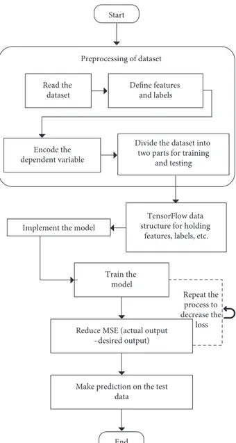
Figure 1 illustrates the steps performed to predict market direction by using the TensorFlow framework. It starts with preprocessing step that extracts features and performs normalization. While reading the dataset, a set of features and labels are defined. If there are string variables, they are encoded. After this step, the dataset is divided into two parts as training and testing datasets. Time series k-fold
cross-validation method is used for evaluation. In this study,
k-fold is set to ten. Financial time series data is split into two
parts as shown in Figure 2. In each cross-validation step, the training data gets bigger and includes all data prior to the testing data whereas the size of testing data stays the same. In the last cycle of cross-validation, the size of the training dataset is nine times bigger than that of the test dataset. After the formation of a model with the training dataset at each step, the model is tested with the testing dataset and pre-cision, accuracy, cumulative return, maximum drawdown, and return on investment are calculated. Here, the ultimate goal is to achieve the highest precision, accuracy, cumulative return, and the lowest maximum drawdown. Hence, optimal parameters are obtained based on the trade-off between accuracy and cumulative return.
3.1. Classification Methods. In this study, four types of data
mining algorithms were used to compare the financial
forecasting capabilities of the models. This section gives a brief description of the classification approaches which we have used.
3.1.1. DNN Classifier. A Multilayer Perceptron (MLP) is
composed of one input layer, one or more hidden layers, and one output layer. Every layer except the output layer includes a bias neuron and is fully connected to the next layer. When an ANN has two or more hidden layers, it is called a Deep Neural Network (DNN) [47].
For creating fully connected neural network layers, handy functions of TensorFlow are used. The DNNClassifier calls tf.estimator.DNNClassifier from the TensorFlow Python API [46]. This command builds a feedforward multilayer neural network that is trained with a set of labeled data in order to perform classification on similar, unlabeled data. As an activation function, we used ReLU and also regularization and normalization hyperparameters are optimized.
The flexibility of neural networks is also one of their main drawbacks since there are many hyperparameters to tweak. Apart from using it in any imaginable topology, one can use it even in a simple MLP, where the number of layers, neurons per layer, the type of activation function used in each layer, the weight initialization logic, and many other parameters can be modified. Therefore, on choosing the best combination of hyperparameters for the DNN model, both grid search and randomized search are used. Since Grid-SearchCV evaluates all combinations, it can take a long time to find the best hyperparameters. For that reason, the hyperparameter adjustment process for DNN is carried out in two steps. First, RandomizedSearchCV is used to narrow the range for each hyperparameter. Than GridSearchCV is implemented using a grid based on the best values provided by the RandomizedSearchCV.
Fitting parameters that are used for Random-izedSearchCV are as follows: “n-neurons”: [64, 128, 256, 512, 1024, 2048]; “n-hidden layers”: [3, 4, 5, 6, 7, 8]; “batch size”: [10, 50, 100, 200]; “learning rate”: [0.01, 0.02, 0.05, 0.1]; “activation”: [tf.nn.relu, tf.nn.elu, leaky-rela (alpha � 0.01),
0 1 2 3 4 5 6 7 8 0 20 40 60 80 100 Sample index CV interation Testing set Training set
Figure 2: Cross-validation time series split. Start End Repeat the process to decrease the loss TensorFlow data structure for holding
features, labels, etc. Implement the model
Read the dataset Define features and labels Preprocessing of dataset Encode the dependent variable
Divide the dataset into two parts for training
and testing
Train the model
Reduce MSE (actual output –desired output)
Make prediction on the test data
leaky-relb (alpha � 0.1)]; “optimizer class”: [tf.train.Ada-mOptimizer, partial (tf.train.MomentumOptimizer, momentum � 0.95)]; and “dropout rate”: [0.2, 0.3, 0.4, 0.5, 0.6].
By using RandomizedSearchCV even if it is not tested every combination, a wide range of values is tested ran-domly. Since balancing time versus performance is of the main concerns, on defining RandomizedSearchCV test parameters, we were trying to increase the performance on limited time. For this, n-iter—number of parameter set-tings that are sampled—is set to 80. And also cv—number of folds to use for cross-validation—is set to 4. By in-creasing these parameters may increase the performance but also increases the run time. Best hyperparameters obtained from fitting the RandomizedSearchCV are as follows: “hidden units” � [1024, 512, 256]; “n-hidden layers”: 3; “batch size”: 50; “learning rate”: 0.05; “activa-tion”: tf.nn.relu; “optimizer class”: tf.train.AdamOptim-izer; and “dropout rate”: 0.5.
To improve DNN performance, GridSearchCV is used by focusing on the most hopeful hyperparameters from RandomizedSearchCV. Fitting parameters that are used for GridSearchCV are as follows: “n-neurons”: [128, 256, 512, 1024]; “n-hidden layers”: [3, 4, 5]; “batch size”: [40, 50, 60]; “learning rate”: [0.04, 0.05, 0.06]; “activation”: [tf.nn.relu, tf.nn.elu]; “dropout rate”: [0.4, 0.5, 0.6]; and “optimizer class”: [tf.train.AdamOptimizer, partial (tf.train.Momentu-mOptimizer, momentum � 0.95)].
After fitting, the GridSearchCV best hyperparameters for the DNN model are obtained. Obtained hyperparameters are as follows: “hidden units” � [1024, 512, 512, 128]; “batch size”: 60; “learning rate”: 0.06; “activation”: tf.nn.relu; “optimizer class”: tf.train.AdamOptimizer; “dropout rate”: 0.4; and “n-classes” � 2.
3.1.2. Logistic Regression. In predicting the direction of the
market, Logistic Regression is generally used to estimate the likelihood of a sample belonging to a particular class. For making it a binary classifier, the model predicts that the instance belongs to that class if the estimated probability is greater than 50%; otherwise, it does not.
Vectorized form of Logistic Regression model esti-mated probability is shown in equation (1). Logistic Re-gression model is computed by adding bias term to weighted sum of the input features, resulting as logistic outputs. As shown in equation (2), the logistic, also called the logit, is a sigmoid function that outputs a number between 0 and 1:
p � hθ(x) �σ θ T· x, (1)
σ(t) � 1
1 + exp(−t). (2) After probability p � hθ(x) has been estimated by Lo-gistic Regression model, prediction y can be calculated easily using equation (3). When θT· x is positive, the model predicts as 1 (rise), and otherwise, it predicts 0 (fall):
y � 0, if p< 0.5,
1, if p≥ 0.5.
(3)
The aim of the training is to set the parameter vector θ, so that the model estimation is maximized. For this purpose, a cost function is used. The cost function over the whole training set is simply the average cost over all training in-stances. Since the cost function is convex, using Gradient Descent guarantees the finding of the global minimum [47]. To implement LR, Scikit-Learn Logistic Regression model is used. For model regularization, ℓ1and ℓ2 penalties are implemented. On Scikit-Learn, ℓ2 penalty is added by default [48].
Even though hyperparameters are not so critical on LR, we wanted to be sure that we are using the best hyper-parameters for our dataset; therefore, the hyperhyper-parameters are tuned. The best model was chosen by using the Grid-SearchCV by defining the grid of the parameters desired to be tested in the model. Useful differences in performance or convergence with different solvers may be seen. Therefore, “newton-cg,” “lbfgs,” and “liblinear” solvers have been added to the grid to be tested. As penalty (regularization), ℓ1 and ℓ2 parameters are used. Finally, C parameter is added to the gird, which controls regularization strength. As C pa-rameters, 100, 10, 1.0, 0.1, and 0.01 values are used. Obtained best parameters for LR after running GridSearchCV are
C � 0.01, penalty � “l2,” and solver � “liblinear.”
3.1.3. Random Forest. Decision trees are one of the widely
used machine learning methods to predict the direction of the stock market. Since there are extremely irregular pat-terns, trees need to grow very deep to learn these patpat-terns, which can cause trees to overfit training sets. A slight noise in the data can cause the tree to grow in a completely different way. The reason for this is that decision trees have very low bias and high variance. Random Forest overcomes this problem by training multiple decision trees on different subspace of the feature space at the cost of slightly increased bias [34]. The Random Forest algorithm introduces extra randomness when growing trees; instead of searching for the best feature when splitting a node, it searches for the best feature among a random subset of features [47]. This means none of the trees in the forest sees the entire training data. The data are recursively split into partitions. At a particular node, the split is done by asking a question on an attribute. The choice for the splitting criterion is based on some impurity measures such as Shannon Entropy or Gini im-purity. This results in a greater tree diversity, which trades a higher bias for a lower variance, generally yielding an overall better model.
In the implementation of RF, Scikit-Learn Random-ForestClassifier Python library is used [48]. As recom-mended by Breiman Random Forest classifier is trained with 500 trees, each limited to maximum 16 nodes [49]. To improve Random Forest Classifiers performance, hyper-parameters are tuned using a grid search.
There are more than fifteen parameters that can be tuned. We were focused on the most important five of these
parameters. Parameters that are placed on the grid are number of trees in the forest—n-estimators: [100, 200, 300, 400]; maximum depth of the tree—max-depth: [50, 60, 70, 80, 90]; min number of samples required to split an internal node—min-samples-split: [8, 10, 12]; min number of samples required to be at a leaf node—min-samples-leaf: [3, 4, 5]; and the number of features to consider when looking for the best split—max-features: [2, 3]. After the grid search is fitted to the data, best parameters are obtained. Obtained best parameters that are used in this research are n-estimators � 200; max-depth � 60; min-samples-split � 12; min-samples-leaf � 5; and max-features � 3.
3.1.4. Support Vector Machines. For assigning new unseen
objects into a particular category by training a model, SVM is one of the most used binary classifiers. The main idea of SVM is to establish a decision boundary (hyperplane) in which the correct separation of rising and falling samples is maximized [50]. A hyperplane of n-dimensional feature vectors x � x1, . . . , xn can be defined as in equation (4) where the sum of the elements will be greater than 0 on one side and less than 0 on the other:
β0+β1X1+ · · · +βnXn�β0+
n i�1
βiXi�0. (4)
The class of each point xican be denoted by yi∈ 1, −1{ } where y � β0+
n
i�1βiXi. By maximizing the distance be-tween the boundary and any point, we can get an optimal hyperplane. The best data splitting boundary is called maximum margin hyperplane. Data points close to the hyperplane are known as a Support Vector Classifier (SVC), and only these points are relevant to hyperplane selection. SVC cannot be applied to nonlinear functions. For solving this issue in SVM, a more general kernel function is applied as in equation (5) which is a quadratic programming (QP) optimization problem with linear constraints and can be solved by using standard QP solver:
f(x) �sgn β0+ n i�1 αiyiK x, xi ⎛ ⎝ ⎞⎠. (5)
SVM is implemented through Pedregosa et al. Scikit-learn Python library using LinearSVC package [48]. Line-arSVC implements “one-vs-the-rest” multiclass strategy; since we have only two classes, only one model is trained. In order to improve the performance of SVM, we are focused on tuning three major hyperparameters. Kernels, Regularisation, and Gamma are the most important pa-rameters that affect performance. These papa-rameters are placed on the grid in order to be used by GridSearchCV for grid search. The model is evaluated for each combination of algorithm parameters specified in the grid. Used hyper-parameters are as follows: C: [0.1, 1, 10, 100], gamma: [1, 0.1, 0.01, 0.001], and kernel: [rbf, poly, sigmoid]. After fitting GridSearchCV in the training data, the best estimators are acquired. Obtained best hyperparameters that are used in this study are C � 10, gamma � 0.1, and kernel � rbf.
3.2. Dataset. In this study, nine years of BIST 100 index data
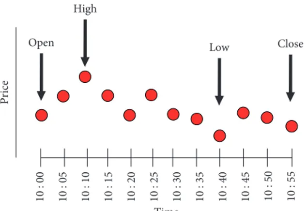
ranging from January 2008 to December 2016 is obtained from Borsa Istanbul Datastore [51]. Although the BIST 100 data in the last few years are published with a time period of one second, the time period in the data we have obtained is ten seconds. Open-high-low-close (OHLC) prices were used to convert the dataset from ten seconds to different time periods. The conversion process is shown in Figure 3. Since dataset is converted from a lower time period to higher time periods, it can be inferred that there is not any missing data in the converted time periods.
For example, in the process of converting to an hourly dataset, the price at the beginning of the hour is taken as open price, maximum and minimum values at that hour are used as high and low prices, and the last price value of the hour is used as close price. In the same way, all the volumes in the hour were agglomerated and the total volume of that hour was obtained. We used open, high, low, and close prices and volume of index data within two hours, hourly, and 30 min periods. Bihourly, hourly, and 30 min datasets are composed of 9157, 18314, and 33673 rows, respectively. An example of hourly dataset is shown in Table 1. For each cross-validation k-fold value, in-sample period is used for training and out-of-sample period is used for evaluating forecasting performance.
When publications about stock predictions are reviewed, it is observed that technical indicators used in technical analysis are generally utilized to generate feature sets of prediction models [52]. Technical indicators are mathe-matical calculation methods used to analyze the prices of financial instruments. After some specific calculations on time series data, most of the indicators help investors to forecast price movement trends in the future. Some indi-cators, on the other hand, try to show whether a trend will continue or not. Indicators are calculated for a specific moment and period to enlighten the investors.
There are literally hundreds of technical indicators that can be used for forecasting. Some of these indicators extract similar information and produce similar signals. The se-lection of the right and diverse set of indicators is important so that a diverse set of measures/indicators can be used as features in the formation of prediction models. The names and descriptions of the selected technical indicators used in the study are given in Table 2. Similar abbreviations have been used for the definition of indicators in Kumar’s et al. [53] and G¨und¨uz’s et al. [54] studies. We use the same naming conventions in this study.
After the selection of the technical indicators, we have to determine time periods and required OHLC price data to be used in the calculation of these indicators. For example, the SMA, EMA, ROCP, and MOM indicators were calculated using the closing price of the BIST 100 index and on 3, 5, 10, 15, and 30 previous values of time series on two hour, hourly, and 30 min interval periods. The WILLR, CCI, UO, and ATR indicators were found using the daily maximum, minimum, and closing prices of the BIST 100 index. These values are calculated using 4 time periods for WILLR, and one time period for CCI, UO, and ATR. With the calculation of different indicators for different time periods, we obtained
97 features for each period of the BIST 100 index. After the features are composed, min-max normalization is applied to each feature as in equation (6) where x � x1, . . . , xn
expresses feature vectors and z is the normalized value of x. The dataset obtained was used for each model; there is no change in the dataset according to the models:
zi� xi−min(x)
max(x) − min(x). (6) In this study, class labeling is determined based on returns calculated according to the closing prices of the BIST 100 index’s trading periods. ri symbolizes the return of the i-th trading period and r(i+1)symbolizes the return of the next
trading period where trading periods are defined as thirty minutes, one hour, and two hours, respectively. Also pi denotes the closing price of i-th trading period and p(i+1)
denotes the closing price of the next trading period as it is used in the following equation:
r(i+1)�p(i+1)− pi
pi . (7)
The class label for i-th period, i.e., yR
i for Rise and yFi for Fall, is set based on the following equations:
yRi � 1, If r(i+1)> r(i)+θ, 0, otherwise, (8) yFi � 1, If r(i+1)< r(i)−θ, 0, otherwise. (9)
In the class labeling equations, the threshold value θ is used to arrange transaction costs and define targeted returns. Due to the transaction costs and risk of a stock exchange, investors are not willing to do too many transactions, at least the transaction costs are targeted to be met. In order to be able to take off from the transactions where the return is less than the transaction cost and also to be able to evaluate the success of the system according to prediction performance and compound return, different threshold values are used. They were obtained from multiplying the standard deviation of returns by predetermined values. Predetermined values start from 0 and increase by 0.1 until they reach 0.5. In this way, six different threshold values were obtained.
3.3. Performance Measures and Implementation of Prediction Model. Predicting the market direction, whether it moves
upside or downside, is equally important since traders can make a profit from both sides. Therefore, predicting index rise and index fall is modeled separately. In the first model, the system is trained to predict whether there will be a rise or not, and in the second model, the system is trained to predict whether there will be a fall or not. In order to overcome the transaction costs problem, we have used a dynamic threshold variable which helps us to eliminate small returns that are less than transaction costs. Evaluation metrics are needed to measure and compare the predictability of clas-sifiers. To evaluate the performance and robustness of the proposed models, we have used performance metrics that are derived from confusion matrix like accuracy, precision, and recall. To evaluate the model’s performance from a fi-nancial return perspective, we have used compound return
Table 2: Selected technical indicators.
Name Description
OPP Opening price of period
HPP Highest price of period
LPP Lowest price of period
CPP Closing price of period
ROC (x) Rate of change of closing price
ROCP (x) Percentage rate of change of closing price
%K Stochastic oscillator
%D Moving average of % for x period
BR Bias ratio
MA (x) Moving average of x periods
EMA (x) Exponential moving average of x periods
TEMA (x) Triple exponential moving average of x periods
MOM (x) Momentum
MACD (x, y) Moving average convergence divergence of x
periods
PPO (x, y) Percentage price oscillator
CCI (x) Commodity channel index
WILLR (x) William’s %
RSI (x) Relative strength index
ULTOSC (x, y, z) Ultimate oscillator
RSI (x) Relative strength index
RDP (x) Relative difference in percentage
ATR (x) Average true range
MEDPRICE (x) Median price
MIDPRICE (x) Medium price
SignalLine (x, y) Signal/trigger line
HHPP (x) Highest closing price of last x periods
LLPP (x) Lowest closing price of last x periods
10 : 00 10 : 05 10 : 10 10 : 15 10 : 20 10 : 25 10 : 30 10 : 35 10 : 40 10 : 45 Open High Low Close Price Time 10 : 50 10 : 55
Figure 3: Conversion of ten seconds time period BIST 100 data to hourly OHLC.
Table 1: BIST 100 hourly data structure.
Date Open High Low Close Volume
2008010209 55160.20 55171.04 54889.51 54951.62 180514
2008010210 54891.50 55281.66 54821.49 54854.45 132182
2008010211 54853.80 54951.23 54481.52 54638.57 76451
2008010212 54527.59 54527.59 54527.59 54527.59 25427
and return of investment metrics. Additionally, max drawdown measurement is used for evaluating the model’s risk of investment.
3.3.1. Confusion Matrix. In machine learning algorithms,
classifiers’ performance evaluation is mainly done by the confusion matrix. The number of true and false estimates is summarized by the counting of values separated by each class. It provides a simple way to visualize the performance and robustness of an algorithm.
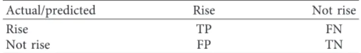
Since we aim to estimate gains that cover transaction costs and focus on eliminating small returns, we use the threshold structure as shown in equations (8) and (9). For the evaluation of upward movement predictions, the con-fusion matrix is shown in Table 3. And also for evaluating downward movement predictions, the confusion matrix is shown in Table 4. For upward movement, positive obser-vation is Rise and negative obserobser-vation is Not Rise. Similarly, for downward movement, positive observation is Fall and negative observation is Not Fall.
Assessments of performance and robustness of the proposed models are calculated based on these four values of the confusion matrix. Accuracy, precision, recall, and F-score are among important measures which are calculated from these values.
Accuracy percentage calculation is given in equation (10). Since accuracy measures true orders and our dataset is unbalanced, only the model evaluation by accuracy will not be enough:
accuracy% � TP + TN
TP + TN + FP + FN×100. (10) In the trading model, false positive (FP) means that actually there is no opportunity for profit, but the model indicates that you need to enter into trade (buy or sell). In this case, you will lose money, which is the worst possible situation. Thus, choosing a model with minimum FP is crucial. This can be achieved by maximizing precision. The calculation of the percentage of precision is shown in the following equation:
precision% � TP
TP + FP×100. (11) On the other hand, false negative (FN) means that al-though there is an opportunity to make money from trade, the model does not indicate that. In this case, the oppor-tunity to make money will have escaped, but it will not be perceived as a major problem as there is no expectation in trading to predict every movement of the market. Recall maximization indicates FN minimization. Percentage of recall calculation is shown in the following equation:
recall% � TP
TP + FN×100. (12) Lastly, the F-score provides insights for the relation between precision and recall. Since precision and recall are prioritized equally, F1-score is used as F-score. The following equation provides definitions of F1-score:
F1 − score �2 × precision × recall
precision + recall . (13)
3.3.2. Compound Return. Calculating the rate of return of
our predictions correctly is one of the main concerns, since we are assuming to put all investment without excluding profit or compensate losses, in each trade. The compound return is one of the best measurement tools that fit for this purpose. Shown as a percentage, compound return indicates the outcome of a series of profits or losses on the initial investment over a while, in a continuous manner.
When evaluating the performance of an investment’s return over a time period, it is known that average return as a measurement tool is not as proper as compound return. This is because when the average return is used, the returns are independent of each other and the effect of each return cannot be carried on to the next step, resulting in failure to clearly determine the success of the model. For average return calculation, discrete returns can be used. Discrete returns are calculated as shown in equation (14), where Pt represents the price at time t and Pt+1represents the price at
time t + 1:
PEd(t, t +1) �
Pt+1
Pt −1. (14)
When calculating the average return, discrete returns are summed and divided by the number of periods. The return of the aggregated multiperiod performance will only be correct if period returns are contributed. Since discrete returns are multiplicative, they will not be appropriate in this case. Thus, the correct aggregated performance is calculated using the compound return formula as shown in the fol-lowing equation [55]:
PEd(0, T) � T−1 0
1 + PEd(t, t +1) − 1. (15)
At the beginning of each period, trained models decide whether to enter the trade. If it enters a trade, at the end of the period, the trade closes. For each trade, discrete return is calculated. This means, if it is traded on the hourly time period, at the beginning of the hour, the model decides whether it should open an order a not. And at the end of the hour, the model closes the open order.
Table 3: Confusion matrix of upward movement.
Actual/predicted Rise Not rise
Rise TP FN
Not rise FP TN
Table 4: Confusion matrix of downward movement.
Actual/predicted Fall Not fall
Fall TP FN
3.3.3. Maximum Drawdown. The main concerns of the
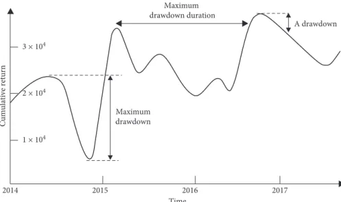
investment are capital protection and consistent estimations. Since maximum drawdown (MDD) is one of the most important measures of risk for a trading strategy, it plays a crucial role in evaluating the performance of the prediction model [56]. MDD value is calculated as shown in the fol-lowing equation:
MDD �P − L
P , (16)
where P represents peak profit before largest loss and L represents the lowest value of loss before the new profit peak is established.
MDD is used to express the difference between the highest capital level and the lowest capital level, where the highest capital level must occur before the lowest capital level. The maximum drawdown duration is the longest time it takes for the forecasting model to recover the capital loss [57]. MDD structure has been illustrated in Figure 4. In this study, drawdowns are measured in percentage terms.
4. Experimental Results
Supply and demand helps to determine the price of each security or the willingness of participants—investors and traders—to trade. Buyers, in exchange, offer a maximum amount they would like to pay, which is usually lower than the demand of the sellers. In order a trade to take place, either buyer increases the price or seller reduces the price. According to this, if the purchase occurs, the price increases and the price decreases if sales are made. This shows that the decision of the investors has a direct effect on the price.
As mentioned before, we know that traders use technical analysis methods in decision making. The main idea in this study is that if the market’s direction of movement is shaped by traders’ transactions [2], and if the majority of traders are using technical analysis methods in the decision-making process [8], by training deep learning and classic machine learning methods using technical analysis indicators to es-timate the market direction, we are actually modeling traders’ behavior.
To strengthen this idea, first of all, we had to choose the best timeframes. We started with examining high-frequency trading (HFT) studies [58]. In these studies, the processing time ranged from milliseconds to seconds, and we observed that market makers frequently use these strategies. As we do not have an appropriate infrastructure, we have decided that these methods will not be applicable to us because the transactions to be made within these periods will not cover the costs.
In addition, we investigated studies, in which deep learning and machine learning methods have been suc-cessfully applied. These studies attempt to predict a wider time frame, such as weekly, monthly, or annual estimates [30]. We did not find appropriate to use these time intervals because the sample size decreased dramatically in these studies. We think that predicting for such long horizons would be too risky.
After a long process of literature review, we decided to focus on intraday intervals rather than daily, weekly, or monthly time periods. Our decision is based on the fact that the vast majority of recent studies are focusing on intraday trading research. Also, their cumulative returns are higher than larger timeframes. These facts are the main reasons for focusing on an intraday investigation. In addition, being less risky is another important factor that forced us to examine intraday market direction prediction.
In order to compare the performance of classification techniques according to the prepared dataset, four different machine learning methods were used in three different time periods and bidirectional (buy/sell) operations were tested on six different threshold values, resulting in a total of 144 aspects. To avoid the problem of overfitting which may arise while designing a supervised classification model for pre-dicting the direction of the index, k-fold cross-validation is applied to each aspect where k value is set to ten. In the strategies applied according to the methods of deep learning and machine learning, there are 48 different results in each period. In the obtained results, the threshold value was tested with a total of six different threshold values starting at 0 up to 0.5, with incremental steps of 0.1.
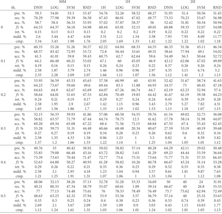
The detailed evaluation of the BIST 100 index direction forecast performance concerning rise and fall is listed in Tables 5 and 6, respectively. We compare the predictive performance of Deep Neural Network (DNN), Support Vector Machine (SVM), Random Forest (RF), and Logistic Regression (LR) on the out-of-sample test set in terms of confusion matrix values, accuracy (acc. %), precision (pre. %), recall (rec. %), and the F1-score (f1 %). Also we added maximum drawdown (mdd. %) and compound return (cmp.) on performance evaluation metrics.
It may be misleading to use only traditional machine learning performance assessment measures to evaluate the trading model estimate. For trading applications, higher accuracy in estimates does not always mean higher profits. Any trading strategy will ultimately lose money, even if the strategy appears to be profitable on paper if the returns are not high enough to come up above the transaction costs associated with commissions, spreads, and slips in a series of consecutive transactions. In a particular way, parameters such as threshold value, average return per transaction, maximum drawdown, and cumulative return represent a more appropriate measure for such a study [23].
Our main target was to investigate whether if it is possible to predict the BIST 100 index consistently using deep learning and machine learning classification ap-proaches. For supporting decisions on financial markets, results are compared with the “buy and hold” strategy. Since the average return of the “buy and hold” strategy on the BIST 100 index on the test period is %15, from the results in Tables 5 and 6, it can be seen that compound return of both DNN and other methods outperform buy and hold strategy. From Tables 5 and 6, it can be pointed out that the outcome acquired by the average 10-fold cross-validation seems to demonstrate the inverse correlation between ac-curacy and compound return. For instance, in Table 5 considering threshold values ranging from 0 to 0.5 for the
DNN, it can be noticed that precision and compound return (cmp.) decreases from 60 to 48 and from 3.34 to 1.12 whereas accuracy and average return (ret.) per trade increases from 58 to 77 and from 0.15 to 0.33, respectively. Additionally, by increasing the time period from 30 min to 2 hours, com-pound return decreases. The reason for the increase in ac-curacy and decrease in compound return is that by increasing the threshold value, we are aiming to minimize risk and to maximize return per trade. Results indicate that we are reaching our goal of minimizing the number of trades and increasing return per trade. By targeting larger returns, we reduce the number of transactions and eliminate smaller returns, which results in a reduction of compound return. The numbers of correct predictions though are increasing and likewise accuracy increases. Recall decreases as we are limiting the number of trades.
Similar results can be seen in Table 6 where fall direction is predicted. As expected, DNN performs better in smaller time periods where there are more records. By decreasing the number of instances, DNN performance decreases. On the other hand, the performance of Random Forest and SVM increases. By using threshold and time period struc-ture, we are enabling investors to weigh the potential reward against the risk to decide if the pain is worth the potential gain.
The results obtained for predicting price rise are reported in Table 5. All models were compared according to the test results corresponding to each threshold value. From Table 5, it can be concluded that the highest compound return with minimum drawdown and maximum precision can be achieved with the DNN model.
In order to minimize risk, investors aim to diversify their portfolio. To build it without purchasing many individual stocks, they are investing in index funds instead. Even when financial system suffers from erratic behaviors and high volatility, it reflects as a loss to investors. Figures 5 and 6 compare BIST 100 index return with our DNN models
return on different time periods when index performs well and when it causes loss.
2009 is one of the most profitable periods of the BIST 100 index in the dataset. In Figure 5, the DNN model’s results are compared with the BIST 100 index return of this period. Furthermore, in Figure 6, the results of the DNN model were compared with the BIST 100 index, which has suffered a loss in 2016. As can be seen from both results, even investing in the index to achieve a diversified portfolio can lead to losses, while a more stable investment instrument can be obtained by investing according to our proposed deep learning and machine learning models. Independently of the index per-forming well or poorly, risks can be minimized while profit increases simultaneously with the proposed model.
In predicting the direction of the BIST 100 index with deep learning and machine learning methods, we have noticed that true-positive trades’ gains are much higher than false-positive trades’ losses. The accuracy and precision of our test results are close to 60%, which means, even when accuracy and precision are close to the 50% level, the system will be profitable since the gains from true-positive trades are greater than the losses from false-positive trades.
In most of the studies where deep learning and machine learning are applied, average return per trade is not evaluated [35, 44, 53]. There are not many studies that include cumulative return in their results [23]; however, we could not find any study where the average return per trade is compared.
As can be seen from Tables 5 and 6, return percentage
ret. % row is positive and it increases when the threshold
value and time period increase. In Table 5, when the threshold value is 0 and the time period is 30 minutes, the return percentage is 0.15, and it increases to 0.74 when the threshold value is 0.5 and the time period is 2 hours. Similarly in Table 6, when the threshold value is 0 and the time period is 30 minutes, the return percentage is 0.19 and it increases to 0.58 where the threshold value is 0.5 and the time period is 2 hours.
2015 2016 2017 Time 2014 3 × 10⁴ 2 × 10⁴ 1 × 10⁴ Cumulative return A drawdown Maximum drawdown duration Maximum drawdown
According to the results, we observe that DNN has a higher average return per transaction. The profit from the right decisions is greater than the loss from the wrong decisions, resulting in a higher compound return. Creating more profit from right decisions compared to the losses incurred from wrong decisions is the main objective of money management. As Druckenmiller, who was manager at Soros’ Quantum Fund, says “I’ve learned many things from George Soros, but perhaps the most significant is that it’s not whether you’re right or wrong that’s important, but how much money you make when you’re right and how much you lose when you’re wrong” [59]. From our results, we can infer that by applying deep learning and machine
learning methods on predicting BIST 100 direction, profits of being right will be greater than the losses of being wrong. From the results, we can see that, in smaller time periods, compound return is bigger and max drawdown is lower. Therefore, by using smaller time periods, we can achieve lower risk and increase profit. We used three different time intervals to compare estimation performance and com-pound return over different time periods. Selection of the time period can be optimized by trying different values, but time period optimization is not the main focus of this study. From our results, we can infer that, by optimizing time period selection, compound return can increase and max drawdown can be decreased.
Table 5: Results of rising direction orders.
30M 1H 2H
th. DNN LOG SVM RND 1H LOG SVM RND DNN LOG SVM RND
0 pre. % 59.3 54.81 53.3 53.47 54.76 52.26 58.52 48.27 51.93 51.4 50.56 51.45 rec. % 70.29 77.98 59.39 56.58 67.43 86.01 47.02 49.77 73.53 70.23 53.67 56.98 acc. % 58.7 58.4 56.33 55.93 57.02 57.87 58.37 56 52.42 51.81 50.34 50.94 f1 % 64.33 64.37 56.18 54.98 60.44 65.01 52.15 49.01 60.88 59.35 52.07 54.08 ret. % 0.15 0.13 0.13 0.13 0.2 0.2 0.2 0.19 0.22 0.22 0.22 0.22 mdd. % 2.6 3.44 4.47 6.04 3.51 2.11 1.54 3.58 7.93 7.95 8.09 11.77 cmp. 3.34 3.43 1.98 1.76 2.05 1.69 1.33 1.42 1.22 1.22 1.02 1.18 0.1 pre. % 60.35 55.26 51.26 50.57 62.22 64.04 68.33 44.55 46.33 51.56 45.11 46.34 rec. % 68.57 83.42 72.95 55.72 72.8 56.44 33.61 49.51 38.61 77.94 49.1 54.02 acc. % 61.5 61.01 59.8 59.43 60.75 62.7 62.64 59.6 54.49 56.3 50.64 52.72 f1 % 64.2 66.48 60.21 53.02 67.1 60 45.05 46.9 42.12 62.06 47.02 49.89 ret. % 0.19 0.16 0.15 0.15 0.26 0.24 0.23 0.22 0.37 0.26 0.26 0.24 mdd. % 2.58 1.87 3.79 2.74 1.46 0.96 0.96 2.97 4.35 5.15 6.74 5.2 cmp. 2.35 2.28 2.09 2.07 1.66 1.11 1.07 1.56 1.12 1.41 1.2 1.13 0.2 pre. % 53.95 56.59 45.53 45.63 57.38 60.99 60 43.91 52.42 51.67 38.74 41.63 rec. % 64.23 73.67 59.66 49.6 69.44 83.5 11.88 44.93 34.57 75 40.45 47.18 acc. % 64.63 64.9 62.67 62.69 64.07 67.26 66.74 64.7 62.19 62.23 52.94 57.4 f1 % 58.64 64.01 51.65 47.53 62.84 70.49 19.83 44.42 41.67 61.19 39.58 44.23 ret. % 0.24 0.21 0.19 0.17 0.29 0.27 0.24 0.24 0.45 0.39 0.29 0.28 mdd. % 2.58 1.95 2.9 2.67 1.42 1.15 0.96 3.43 2.79 5.27 7.82 4.51 cmp. 1.65 1.56 1.86 1.7 1.35 1.19 1.02 1.53 1.13 1.18 1.07 1.15 0.3 pre. % 52.15 56.33 39.93 41.86 57.06 60.58 54.55 39.76 61.54 49.02 32.75 36.08 rec. % 58.82 63.57 71.79 47.44 64.74 78.75 12.5 41.62 17.78 58.14 51.98 44.07 acc. % 69.28 69.34 65.08 67.22 68.4 71.56 71.15 68.84 67.55 67.4 55.43 62.45 f1 % 55.28 59.73 51.31 44.48 60.66 68.48 20.34 40.67 27.59 53.19 40.19 39.68 ret. % 0.27 0.27 0.19 0.19 0.34 0.28 0.23 0.26 0.62 0.6 0.32 0.34 mdd. % 2.58 1.35 4.33 1.58 0.96 1.23 1 3.5 0.82 4 8.59 5.82 cmp. 1.37 1.2 1.66 1.53 1.22 1.14 1 1.25 1.04 1.05 1.01 1.12 0.4 pre. % 49.76 55 40.42 38.92 59.02 58.82 57.14 40.28 64.29 42.11 29.02 30.48 rec. % 55.85 79.08 66.48 43.16 63.72 58.82 5.63 41.29 69.23 44.44 33.59 36.64 acc. % 73.39 73.63 70.44 71.47 72.77 75.6 75.51 73.64 71.77 71.51 57.55 66.45 f1 % 52.63 64.88 50.27 40.93 61.28 58.82 10.26 40.78 66.67 43.24 31.14 33.28 ret. % 0.29 0.26 0.22 0.21 0.35 0.36 0.23 0.29 0.52 0.55 0.35 0.38 mdd. % 2.58 2.1 2.95 4.18 1.23 1.04 0.94 3.57 0.61 1.81 9.87 7.63 cmp. 1.21 1.25 1.91 1.31 1.07 1.06 1 1.33 1.04 1 1.12 1.08 0.5 pre. % 48.06 52.13 38.26 37.13 52.78 51.28 33.33 34.69 50 40 24 31.91 rec. % 49.21 80.33 47.34 38.79 55.07 60.61 1.89 39.14 66.67 40 26.8 35.55 acc. % 77 77.13 74.48 75.61 76 78.53 78.49 76.49 75.7 75.62 62.94 72.49 f1 % 48.63 63.23 42.32 37.94 53.9 55.56 3.57 36.79 57.14 40 25.32 33.63 ret. % 0.33 0.3 0.25 0.24 0.4 0.38 0.23 0.36 0.53 0.74 0.39 0.43 mdd. % 2.69 2.1 3.67 2.09 1.59 1.09 0.9 3.03 0.43 1.15 10.83 1.77 cmp. 1.12 1.24 1.61 1.31 1.05 1.06 1.01 1.24 1.02 1.01 1.05 1.13
One of the most important implications of our results is that deep learning and machine learning methods produce successful results when used in predicting market direction. Our results indicate why large funds and experts are in-volved in using and studying deep learning and machine learning methods to predict financial markets [60].
4.1. Implications from Experiment Results. To summarize the
obtained results, although traditional machine learning techniques are still preferred mainstream methods in pre-dictive analysis, recent research shows that these methods do not capture the properties of complex, nonlinear problems as well as deep learning methods. Accordingly, these
experiments show that a deep learning algorithm, indirectly, has the capacity to produce an appropriate representation of information.
Even though according to the confusion matrix DNN model performs notably better than other models according to compound return, max drawdown, and precision, we aimed to identify if any observed difference is statistically significant. For comparing the statistical significance of the models, McNemar test is used, in which it captures the errors made by both models [61]. The null hypothesis is the ex-pression that classifiers have a similar proportion of errors on the test set. On McNemar test, the p value is below a given threshold (0.05) only on DNN-RF comparison. We can reject the null hypothesis since the p value is 0.048 and infer
Table 6: Results of falling direction orders.
30M 1H 2H
th. DNN LOG SVM RND DNN LOG SVM RND DNN LOG SVM RND
0 pre. % 61.05 60.47 53.98 55.84 62.53 61.97 50.09 49.6 53.52 53.62 49.92 50.17 rec. % 49.11 34.38 47.79 52.72 49.38 22.49 61.47 48.1 30.93 34.14 46.81 44.62 acc. % 57.51 57.69 56.18 57.12 57.64 58.37 57.4 57.15 53.43 54 51.4 51.58 f1 % 54.44 43.84 50.69 54.24 55.18 33 55.2 48.84 39.21 41.72 48.32 47.23 ret. % 0.19 0.18 0.14 0.14 0.31 0.3 0.29 0.2 0.24 0.24 0.23 0.23 mdd. % 2.04 2.47 1.9 2.4 1.97 1.26 3.18 3.35 3.87 4.07 8.08 4.85 cmp. 3.77 3.35 2.59 2.54 2.51 1.32 1.53 1.72 1.31 1.38 1.19 1.12 0.1 pre. % 61.18 61.12 53.39 51 65.04 63.03 52.91 46.66 47.51 53.96 42.26 46.24 rec. % 52.37 27.84 30.89 45.82 53.38 70.09 82.73 41.75 55.4 26.09 38.41 38.74 acc. % 61.14 60.44 60.04 59.73 61.58 62.74 62.33 60.77 56.83 58.42 51.62 55.66 f1 % 56.43 38.26 39.14 48.27 58.63 66.37 64.54 44.07 51.15 35.18 40.24 42.16 ret. % 0.26 0.24 0.17 0.16 0.39 0.4 0.36 0.23 0.32 0.28 0.27 0.27 mdd. % 1.64 2.58 1.83 2.66 1.26 0.84 1.8 2.29 4.23 2.87 6.29 5.72 cmp. 2.39 1.73 1.56 2.13 1.83 1.28 1.22 1.62 1.2 1.2 1.09 1.15 0.2 pre. % 58.8 59.33 49.23 46.15 63.68 66 51.1 42.11 45.81 58.62 37.69 38.62 rec. % 48.22 40.46 35.41 42.24 50.94 37.5 92.08 41.1 63.8 33.55 36.02 33.44 acc. % 64.91 64.67 63.99 63.03 65.27 66.82 66.59 64.14 62.72 64 54.42 58.72 f1 % 52.99 48.11 41.19 44.11 56.6 47.83 65.72 41.6 53.33 42.68 36.84 35.84 ret. % 0.3 0.29 0.2 0.19 0.51 0.5 0.39 0.26 0.41 0.31 0.3 0.3 mdd. % 1.75 1.35 2.46 2.07 0.73 0.71 1.75 2.43 3.03 1.79 6.15 4.31 cmp. 1.72 1.44 1.54 1.8 1.55 1.16 1.28 1.5 1.13 1.14 1.13 1.12 0.3 pre. % 56.25 59.2 51.36 45.36 63.33 54.05 52.81 39.89 40.32 50 35.86 32.4 rec. % 49.51 51.75 21.62 39.84 55.56 32.79 90.38 38.05 83.33 40.91 20.1 25.55 acc. % 69.12 69.01 68.95 67.84 69.6 70.88 70.92 68.73 67.74 68.19 63.55 63.92 f1 % 52.67 55.22 30.43 42.42 59.19 40.82 66.67 38.95 54.35 45 25.76 28.57 ret. % 0.37 0.33 0.23 0.21 0.57 0.55 0.49 0.31 0.5 0.51 0.34 0.35 mdd. % 1.64 1.19 1.17 2.14 1.24 0.74 0.89 3.35 1.14 1.04 3.18 7.89 cmp. 1.46 1.24 1.58 1.6 1.38 1.1 1.19 1.46 1.07 1.07 1.17 1.02 0.4 pre. % 56.08 57.89 45.97 41.77 59.41 57.58 47.24 38.48 75 56.52 30.42 31.73 rec. % 50 30.77 22.54 37.58 54.55 57.58 95.24 37.5 70.59 54.17 26.11 26.06 acc. % 73.25 73.14 72.54 71.75 73.58 75 74.77 72.87 72.15 71.96 61.02 68.11 f1 % 52.87 40.18 30.25 39.56 56.87 57.58 63.16 37.98 72.73 55.32 28.1 28.62 ret. % 0.38 0.35 0.25 0.24 0.56 0.59 0.46 0.33 0.54 0.52 0.37 0.4 mdd. % 1.1 1.19 1.76 2.13 1.24 0.71 1.38 1.26 0.28 1.07 4.24 4.4 cmp. 1.38 1.12 1.47 1.47 1.32 1.11 1.21 1.41 1.06 1.06 1.24 1.07 0.5 pre. % 55.24 60 33.93 39.38 61.25 50 48 40.71 83.33 60 26.93 26.09 rec. % 54.11 28.57 26.14 37.71 59.04 40.63 96 36.18 71.43 60 24.12 23.08 acc. % 76.96 76.92 74.54 75.65 77.17 78.47 78.39 77.35 76.23 76.04 65.77 72.6 f1 % 54.67 38.71 29.53 38.53 60.12 44.83 64 38.31 76.92 60 25.45 24.49 ret. % 0.43 0.4 0.26 0.28 0.62 0.6 0.53 0.39 0.58 0.51 0.4 0.41 Mdd. % 1.1 0.5 1.66 1.8 1.24 0.71 0.97 2.47 0.06 0.76 3.96 3.36 cmp. 1.33 1.14 1.29 1.41 1.26 1.07 1.2 1.41 1.05 1.05 1.19 1.02
that the difference between DNN and RF classifiers is sta-tistically significant. But being stasta-tistically significant does not mean that the trading model will be successful since a large loss will result in multiple winnings. Therefore, on model evaluation, return per trade should be considered.
Our results on market direction prediction suggest that better results are achieved with deep learning than classical machine learning methods. Nevertheless, the complex ar-chitecture of deep learning models must be considered. Even if advanced libraries such as TensorFlow and Keras are used, there is a need for comprehensive understanding and solid experimentation to use such models efficiently.
5. Conclusions
Recent trends have led to an increase in studies of models based on technical indicators, demonstrating that both professionals and individual investors use technical indi-cators. Assuming that most people make their investments according to technical indicators, we can confirm that technical indicators actually show the behaviour of investors. Accordingly, in this study, technical indicators applied to BIST 100 index data were used as input for modeling trader behaviour using deep learning and machine learning methods. 2009 /04 2009 /06 Compound return Date 5 4 3 2 1 2009 /05 2009 /07 2009 /08 2009 /09 2009 /10 BIST 100 return DNN 30M th. 0.0 DNN 30M th. 0.1 DNN 30M th. 0.2 DNN 30M th. 0.3 DNN 30M th. 0.4 DNN 30M th. 0.5
Figure 5: Comparison of one of the most profitable periods of BIST 100 index with the return of 30 min DNN.
2016 /04 2016 /06 Compound return Date 3.0 2016 /05 2016 /07 2016 /08 2016 /09 2.5 2.0 1.5 1.0 BIST 100 return DNN 30M th. 0.0 DNN 30M th. 0.1 DNN 30M th. 0.2 DNN 30M th. 0.3 DNN 30M th. 0.4 DNN 30M th. 0.5
As can be deduced from the test results, the main contribution of this study is enabling traders to make profits even if there is negative news and index loss in the market with the deep learning model developed considering OHLC prices and transaction costs.
In this study, we have compared Deep Neural Network with Support Vector Machine, Random Forest, and Lo-gistic Regression on predicting the direction of BIST 100 index in intraday time periods using different threshold values. To test the robustness and performance of these models, empirical studies have been performed on these machine learning methods in three different time periods. Bidirectional (buy/sell) operations were tested on six different threshold values, resulting in a total of 144 as-pects. To avoid the problem of overfitting, k-fold cross-validation is applied to each aspect where k value is set to ten. Metrics such as accuracy, precision, recall, F1-score, compound return, and max drawdown have been used to evaluate the performance of these models on predicting direction.
Empirical findings suggest the superiority of the pro-posed DNN model on lower threshold values and smaller time periods when evaluated based on compound return, average return per trade, and max drawdown. As threshold value increases, the superiority of DNN model over other machine learning methods reduces. Also by using DNN and machine learning methods, we can achieve a model where the number of true-positive orders is higher than that of false-positive orders. At the same time, average returns per trade of true-positive orders are higher than average losses per trade of false-positive orders.
The findings of this study suggest that even if the precision of the model may be close to 60 percent, the outcome from using the same model is profitable. If it is considered what the results obtained mean in practice to a trader. Six out of ten transactions proposed by the model will be in the right direction and the return of these transactions will be higher than the expense of the faulty transactions. If the investment is fixed, depending on the selected threshold value, if the model earns 100 TL from the correct transactions, it loses 75 TL from the faulty ones. Accordingly, the model will make an average of 600 TL (6 ∗ 100) profit and 300 TL (4 ∗ 75) losses. In total, ap-proximately 300 TL profit will be gained. These transac-tions are expected to take place within a few weeks, depending on the time period to be selected.
Data Availability
The “BIST100” data used to support the findings of this study were supplied by “Borsa ˙Istanbul” under license and so cannot be made freely available. Requests for access to these data should be made to “Datastore-Borsa ˙Istanbul” (https:// datastore.borsaistanbul.com/).
Conflicts of Interest
The authors declare that there are no conflicts of interest regarding the publication of this paper.
Acknowledgments
This work was partially supported by the Scientific and Technological Research Council of Turkey—T ¨UB˙ITAK under grant 115K179 (1001—Scientific and Technological Research Projects Support Program).
References
[1] A. W. Lo and J. Hasanhodzic, The Evolution of Technical
Analysis: Financial Prediction from Babylonian Tablets to Bloomberg Terminals, Bloomberg Press, New York, NY, USA,
2010.
[2] J. J. Murphy, Technical Analysis of the Financial Markets: A
Comprehensive Guide to Trading Methods and Applications,
New York Institute of Finance, New York, NY, USA, 1999. [3] A. O. I. Hoffmann and H. Shefrin, “Technical analysis and
individual investors,” Journal of Economic Behavior &
Or-ganization, vol. 107, pp. 487–511, 2014.
[4] R. T. Farias Naz´ario, J. Lima e Silva, V. A. Sobreiro, and H. Kimura, “A literature review of technical analysis on stock markets,” The Quarterly Review of Economics and Finance, vol. 66, pp. 115–126, 2017.
[5] Q. Lin, “Technical analysis and stock return predictability: an aligned approach,” Journal of Financial Markets, vol. 38, pp. 103–123, 2018.
[6] Y.-H. Lui and D. Mole, “The use of fundamental and technical analyses by foreign exchange dealers: Hong Kong evidence,”
Journal of International Money and Finance, vol. 17, no. 3,
pp. 535–545, 1998.
[7] L. Menkhoff and M. P. Taylor, The Obstinate Passion of
Foreign Exchange Professionals: Technical Analysis, University
of Warwick, Department of Economics, Coventry, UK, 2006. [8] L. Menkhoff, “The use of technical analysis by fund managers: international evidence,” Journal of Banking & Finance, vol. 34, no. 11, pp. 2573–2586, 2010.
[9] I. H. Witten and E. Frank, Data Mining: Practical Machine
Learning Tools and Techniques, Elsevier, Amsterdam,
Neth-erlands, 2nd edition, 2005.
[10] E. Formisano, F. Martino, and G. Valente, “Multivariate analysis of fMRI time series: classification and regression of brain responses using machine learning,” Magnetic Resonance
Imaging, vol. 26, no. 7, pp. 921–934, 2008.
[11] C. Jiang, H. Zhang, Y. Ren, Z. Han, K.-C. Chen, and L. Hanzo, “Machine learning paradigms for next-generation wireless networks,” IEEE Wireless Communications, vol. 24, no. 2, pp. 98–105, 2017.
[12] H. F. Alan and J. Kaur, “Can android applications be iden-tified using only TCP/IP headers of their launch time traffic?” in Proceedings of the 9th ACM Conference on Security &
Privacy in Wireless and Mobile Networks–WiSec’16, vol. 9,
pp. 61–66, Darmstadt, Germany, July 2016.
[13] E. I. Zacharaki, S. Wang, S. Chawla et al., “Classification of brain tumor type and grade using MRI texture and shape in a machine learning scheme,” Magnetic Resonance in Medicine, vol. 62, no. 6, pp. 1609–1618, 2009.
[14] N. M. Ball and R. J. Brunner, “Data mining and machine learning in astronomy,” International Journal of Modern
Physics D, vol. 19, no. 7, pp. 1049–1106, 2010.
[15] W. Zhang, T. Yoshida, and X. Tang, “Text classification based on multi-word with support vector machine,”
Knowledge-Based Systems, vol. 21, no. 8, pp. 879–886, 2008.
[16] D. Pratas, M. Hosseini, R. Silva, A. Pinho, and P. Ferreira, “Visualization of distinct DNA regions of the modern human