Adaptive kernel density estimation with generalized least square cross-validation

Volume 48 (2) (2019), 616 – 625

Research Article

Adaptive kernel density estimation with

generalized least square cross-validation

Serdar Demir∗†

Abstract

Adaptive kernel density estimator is an efficient estimator when the density to be estimated has long tail or multi-mode. They use varying bandwidths at each observation point by adapting a fixed bandwidth for data. It is well-known that bandwidth selection is too important for performance of kernel estimators. An efficient recent method is the generalized least square cross-validation which improves the least squares cross-validation. In this paper, performances of the adaptive kernel estimators obtained based on the generalized least square cross-validation are investigated. We performed a simulation study to inform about performances of the modified adaptive kernel estimators. For the simulation, we use also the bandwidth selection methods of normal reference, least squares cross-validation, biased cross-validation, and plug-in methods. Simulation study shows that the adaptive kernel es-timators improve the performances of the kernel eses-timators with fixed bandwidth selected based on generalized least square cross-validation. Keywords: Kernel density estimation, Adaptive bandwidth, Cross-validation.

Mathematics Subject Classification (2010): 62G07

Received : 10.01.2018 Accepted : 19.09.2018 Doi : 10.15672/HJMS.2018.623

1. Introduction

The kernel density estimation (KDE) is the most popular non-parametric method to estimate density function of a distribution. Let X1, X2, ..., Xn be randomly chosen

sample from a population with unknown probability density function f (x). The KDE for density function for any estimation point x is given as

(1.1) fˆh(x) = 1 n n ∑ i=1 1 hk ( x− Xi h )

∗_{Mugla Sitki Kocman University, Faculty of Science, Dep. of Statistics, Mugla, Turkey.}

Email: serdardemir@mu.edu.tr

where h is called as bandwidth or smoothing parameter which controls the smoothness of function. The choice of h is crucial. In Equation (1.1), k(.) is the kernel function which is assumed to satisfy following properties

∫ _∞ −∞ k(u)du = 1, ∫ _∞ −∞ uk(u)du = 0, ∫ _∞ −∞ u2k(u)du = µ2(k) <∞

The selection of kernel function is not as important as the selection of bandwidth and such selection is made by taking into consideration of the ease of calculation and differentiability features. Some popular kernel functions are Gaussian, Epanechnikov, Triangular, Quartic, and Triweight [9].

The mean squared error (MSE), the mean integrated squared error (MISE), and the asymptotic MISE of KDE is follows as

(1.2) MSE ( ˆf (x)) = f (x)R(k) nh + h4 4 { f′′(x)µ2(k) }2 + o((nh)−1) + o(h4) (1.3) MISE ( ˆf ) = ∫ M SE ( ˆf (x)) dx = (nh)−1R(k) +h 4 4 { µ2(k)} 2 ∫ _∞ −∞{f ′′ (x)}2dx + o((nh)−1) + o(h4) (1.4) AMISE ( ˆf (x)) = (nh)−1R(k) +h 4 4 { µ2(k)} 2 ∫ _∞ −∞{f ′′ (x)}2dx

where R(k) =∫k2(u) du [9, 13, 20]. The optimal bandwidth value which minimizes the AMISE is obtained as follows,

(1.5) hopt= [ R(k) nµ2 2(k)R{f′′(x)} ]1/5

To compute hoptapproximately, there are the most widely-used methods such normal

reference (NR), least squares cross-validation (LSCV), biased cross validation (BCV), and plug-in. Basic idea of these approaches is to use the estimations of unknowns. The issue that which one is the best is still controversial. Generally, it is determined which method works well heuristically and through experience in practice. In section 2, the basic properties of the most common fixed bandwidth selection methods are given. In section 3, the adaptive bandwidth selectors are introduced. We will give comparisons of performances of the selectors based on Monte Carlo simulations in section 4. In section 5, a real-data example is presented. Section 6 gives the conclusions.

2. Fixed bandwidth selectors

The simplest method for selecting a bandwidth h is to use the normal reference band (hN R). If f and k are assumed to be a normal distribution and a Gaussian kernel in

Equation (1.5) respectively, then hoptbecomes hN R as follows

(2.1) hN R= 1.06σn−1/5

or alternatively

where σ and IQR are the standard deviation and the interquartile range of X, respectively [13, 16, 17]. By combining Equation (2.1) and Equation (2.2) and using the estimations of σ and IQR, a better normal reference bandwidth is obtained as

(2.3) ˆhN R= 1.06 min(ˆσ, I ˆQR/1.34) n−1/5

It is well-known that ˆhN R works well if f approaches to normal distribution.

Oth-erwise, it often obtains oversmooth estimations, specially in case of multi-modality [9, 16, 17, 20]. Recently, Zhang [21] proposed a robust simple and quick bandwidth selector ˆ

hN R(p) based on quantile for kernel density estimation. Even Zhang [21] states that

ˆ

hN R(0.75) is a good choice of adaptive bandwidths by using the results of the simulation

studies, but it is controversial.

As an automatic method, LSCV which also is called as unbiased cross-validation (UCV ) is a flexible and easy computable method. In LSCV, the optimal bandwidth

ˆ

hLSCV = arg min

h LSCV (h)

which minimizes the following cross-validation function LSCV (h) over h is follows

(2.4) LSCV (h) = ∫ ˆ fh2(x)dx− 2 n n ∑ i=1 ˆ fh(i)(Xi) where ∫ ˆ fh2(x)dx = 1 n2_h n ∑ i=1 n ∑ j=1 (k∗ k) ( Xi− Xj h ) In Equation (2.4), ˆ fh(i)(Xi) = 1 (n− 2)h n ∑ j̸=i k(Xi− Xj h )

is a leave-one-out kernel estimator that is computed from the sample points by ignoring

Xi [2, 9, 14, 20]. LSCV bandwidth estimator is unbiased but highly variable depending

on selected sample and often produces undersmooth estimations [4, 8, 12].

Differently from LSCV, BCV method is based on AMISE . The BCV bandwidth ˆ hBCV = arg min h BCV (h) is the minimizer of BCV (h) = R(k) nh + h4 4{µ2(k)} 2_ˆ R(f′′) where ˆ R(f′′) = 1 (nh)2 n ∑ i̸=j (k′′∗ k′′)(Xi− Xj h )

is a estimator of R(f′′) and k′′is the second derivative of k [9, 20]. Scott and Terrell [14] showed that ˆhBCV is more stable than ˆhLSCV but a biased estimator. Chiu [4] stated

that ˆhBCV does not work for small sample sizes. Zhang [21]’s simulation studies showed

that the minima of LSCV and BCV functions sometime occurs at extreme points of h, especially for sharp and multiple peaks.

Basic idea of plug-in bandwidth selectors is plugging in estimates of the unknown quantities in hopt[20]. Sheather and Jones [15] proposed a bandwidth selector ˆhSJ which

is ‘solve-the-equation’ method. Chiu [4] stated that procedure SJ performs quite well for densities close to normal distribution. Loader [11] expressed that “the much touted plug-in approaches have fared rather poorly, beplug-ing tuned largely by arbitrary specification of pilot bandwidths and being heavily biased when this specification is wrong”. Zhang [21] showed ˆhSJ performs well in all cases (unimodal and multimodal).

Recently, a generalized least squares cross-validation (GLSCV) method is proposed by Zhang [22]. This method aims to improve the finite sample behavior of LSCV method. Zhang [22] give the GLSCV function as

LSCVg(h) = ϕ√_2h(0) n + 2 n(n− 1) ∑ i<j [ 2 g(g− 2)ϕ√2h(Xi− Xj)− ( 1 n+ 1 g− 2 ) ϕ√ 2h(Xi− Xj) ]

where Φ(.) is Gaussian kernel and Φh(u)= Φ(u/h)/h. Zhang [22] only discussed LSCV (h)

for Gaussian kernel. When g=1 then LSCVg(h) equals to LSCV (h). The generalized

LSCV bandwidth selector ˆhLSCV gis defined as the minimizer of LSCVg(h) over h. Zhang

[22] stated that “based on our simulation study, the poor finite sample behavior of ˆhLSCV

can be dramatically improved by ˆhLSCV gwith 3≤ g ≤ 4, where g=4 seems to be the best

choice for any sample size n”. Zhang [22] give a script for computing ˆhLSCVg in R code

[5]. By using this code, LSCVg (h) is minimized over h within [0.01ˆhOS, ˆhOS]. Here,

ˆ

hOS = 1.144n−1/5S is the oversmoothed bandwidth selector for Gaussian Kernel where

S is sample standard deviation [20]. In this study, we use also Zhang’s codes located in

our R codes for the simulation study.

3. Adaptive kernel density estimators

It is well known that all the classical bandwidth selection methods perform well if true density is close to normal distribution. Otherwise, they are problematic, specially for long-tailed or multi-moded densities. While a kernel density estimator with fixed bandwidth has performance well about the peak of a distribution, but performs poorly at the tails. It is not easy to find only one bandwidth which is satisfied adequately at peaks and tails of a density. As an efficient solution for handling this issue, it is to use the kernel estimator which has a different bandwidth for each data point. These type of kernel estimators are commonly called as adaptive kernel density estimators (AKDE). Van Kerm [19] states that it is commonly preferred for decreasing the oversmooth/undersmooth effects of the fixed bandwidth to use AKDE. Firstly, Breiman et. al. [3] introduced AKDE as (3.1) f (x) =˜ 1 n n ∑ i=1 1 h(Xi)d k(x− Xi h(Xi) )

where h(Xi) is the variable bandwidth for each data point Xiand d is the number of

dimension. Breiman et. al. [3] suggested that h(Xi) must be taken as being proportional

to the distance from Xi to its kth nearest neighbor. Abramson [1] proposed that h(Xi)

must be proportional to f−1/2(Xi),with f replaced by a pilot estimate,for all dimensions.

The mean squared error (MSE) of ˜f (x) with Abramson’s approach is derived by Jones

[10] for d=1 as follows: MSE( ˜f (x)) ∼= 1 576δ 2 kh 8 A2(x) + (nh)−1S(k)f3/2(x)

where, A(x) = d 4 dx4 [ 1 f (x) ] , δk= ∫ x4k(x)dx, S(k) = 3 2R(k) + 1 4R(xk ′_).

Silverman [17] suggested that h(Xi) must be proportional to (g/ ˆf (Xi))1/2 where g is

the geometric mean of ˆf (Xi) values. Silverman [17] suggested a three-stage algorithm to

compute adaptive kernel estimations.

(1) Compute a pilot estimation ˆf (Xi) by using KDE with a fixed bandwidth h for

all data points.

(2) Compute the local bandwidth factors as λi=

{_ˆ

f(Xi)

g

}_−α and

α is the sensivity parameter which is commonly preferred as 0.5 [1].

(3) Compute the adaptive bandwidths as h(Xi) = hλi and estimate the adaptive

kernel density as (3.2) f˜g(x) = 1 n n ∑ i=1 1 h(Xi) K(x− Xi h(Xi) ) = 1 nh n ∑ i=1 1 λi K(x− Xi hλi )

Hall and Marron [7] and Terrell and Scott [18] showed that the AKDE have higher convergence rate than KDE ’s.

Cula et al. [6] investigated the finite sample performances of the modified adaptive kernel density estimators ˜fg(x), ˜fa(x), and ˜fr(x). The modified adaptive kernel density estimators ˜fa_{(x) and ˜f}r_{(x) use average, a =}∑n

i=1f(Xˆ i)/n, and range ,r = max ˆf (Xi)−

min ˆf (Xi), instead of geometric mean g in Equation (3.2). Cula et al. [6] used the

only LSCV bandwidth selector as fixed bandwidth selector and showed that the modified adaptive kernel density estimators based on LSCV outperform the classical kernel density estimators.

Here, we define new modified adaptive kernel density estimators based on using the the fixed bandwidth selectors NR, BCV, SJ, and LSCV4 as ˆfN R, ˆfBCV, ˆfSJ, and ˆfLSCV4,

respectively.

(1) Let ˜f_{N R}g , ˜f_LSCVg , ˜f_BCVg , ˜f_SJg , and ˜f_LSCVg

4denote the adaptive kernel density

estimators based on adaptive bandwidths obtained by using geometric mean. (2) Let ˜fa

N R, ˜fLSCVa , ˜fBCVa , ˜fSJa , and ˜fLSCVa 4denote the adaptive kernel density

estimators based on adaptive bandwidths obtained by using arithmetic mean. (3) Let ˜fr

N R, ˜fLSCVr , ˜fBCVr , ˜fSJr , and ˜fLSCVr 4denote the adaptive kernel density

estimators based on adaptive bandwidths obtained by using range values. We performed a simulation study to inform about performances of the all above mod-ified estimators.

4. Finite sample performances of the modified adaptive

band-width selectors

Because of theoretical difficulties of the kernel estimators, it is most common method to use Monte Carlo simulations for comparing their performances. We generate 1000 Monte Carlo samples of size n (50, 250, 1000) from the normal mixture model as follows

f (x) = 0.5ϕ(x) + 0.5ϕσ(x− µ)

where µ = 0, 1, 5 and σ = 1, 0.5, 0.1 [22]. Following Zhang [22], we use the ‘direct-plug-in’ (dpi) method for ˆhSJ and Gaussian kernel function for all estimations.

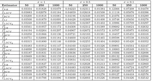
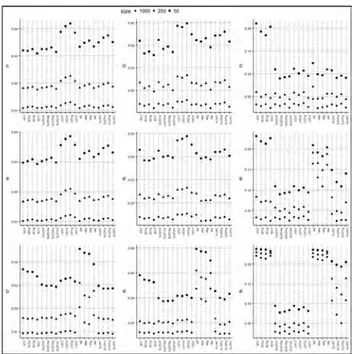
By using generated samples, the root mean integrated square error (RMISE) values of the fixed kernel estimations and the adaptive kernel estimations are computed. For each case, the average values of RMISE’s over 1000 samples are given in Table 1, Table 2, and Table 3. Figure 1 shows the behavior of the RMISE values graphically. It can be concluded the following comments.

As expected, the adaptive kernel density estimators significantly improve the classical kernel density estimators for all cases.

The classical and the adaptive BCV kernel density estimators perform poorly if the true density is sharp or two moded. Otherwise, they perform well. The adaptive BCV estimators often improve the classical BCV estimator.

Table 1. Average RMISE for the case with µ = 0

σ = 1 σ = 0.5 σ = 0.1 Estimator 50 250 1000 50 250 1000 50 250 1000 ˆ fN R 0.03334 0.01828 0.01079 0.04223 0.02311 0.01384 0.12366 0.07208 0.04478 ˆ fLSCV 0.03883 0.02078 0.01184 0.04859 0.02618 0.01508 0.11118 0.05876 0.03396 ˆ fBCV 0.03200 0.01818 0.01081 0.04196 0.02349 0.01395 0.21076 0.06018 0.03289 ˆ fSJ 0.03500 0.01879 0.01095 0.04428 0.02369 0.01400 0.10748 0.05650 0.03278 ˆ f_LSCV4 0.03248 0.01833 0.01089 0.04236 0.02367 0.01402 0.10986 0.05709 0.03297 ˜ f_{N R}g 0.03561 0.01957 0.01172 0.04308 0.02312 0.01389 0.09682 0.04624 0.02632 ˜ f_LSCVg 0.04194 0.02264 0.01297 0.04967 0.02672 0.01572 0.10707 0.05975 0.03582 ˜ f_BCVg 0.03250 0.01866 0.01136 0.03721 0.02183 0.01381 0.18457 0.05455 0.03318 ˜ f_SJg 0.03751 0.02006 0.01184 0.04600 0.02453 0.01465 0.09598 0.05538 0.03432 ˜ fg LSCV4 0.03315 0.01890 0.01146 0.03938 0.02255 0.01404 0.09263 0.05420 0.03352 ˜ f_{N R}a 0.03483 0.01912 0.01147 0.04160 0.02210 0.01326 0.09891 0.04564 0.02447 ˜ f_LSCVa 0.04090 0.02209 0.01268 0.04803 0.02560 0.01501 0.10083 0.05349 0.03151 ˜ f_BCVa 0.03187 0.01831 0.01116 0.03636 0.02097 0.01319 0.19306 0.04955 0.02898 ˜ fa SJ 0.03669 0.01961 0.01159 0.04443 0.02345 0.01399 0.09132 0.04930 0.02996 ˜ f_LSCV4a 0.03251 0.01854 0.01125 0.03834 0.02162 0.01341 0.08992 0.04849 0.02932 ˜ f_{N R}r 0.03347 0.01827 0.01107 0.03912 0.02028 0.01213 0.10947 0.05637 0.02860 ˜ f_LSCVr 0.03853 0.02079 0.01211 0.04483 0.02336 0.01364 0.09559 0.04724 0.02707 ˜ f_BCVr 0.03090 0.01769 0.01089 0.03563 0.01953 0.01210 0.20320 0.04672 0.02520 ˜ fr SJ 0.03509 0.01876 0.01117 0.04160 0.02148 0.01276 0.09127 0.04418 0.02576 ˜ fr LSCV4 0.03148 0.01788 0.01096 0.03698 0.02003 0.01226 0.09408 0.04426 0.02542

The classical generalized LSCV and adaptive generalized LSCV density estimators perform well for all cases. The adaptive estimator ˜fLSCVr 4has generally very attractive

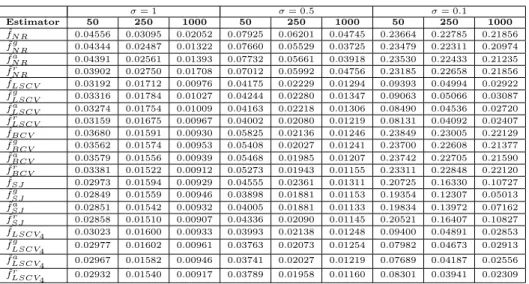
Table 2. Average RMISE for the case with µ = 1 σ = 1 σ = 0.5 σ = 0.1 Estimator 50 250 1000 50 250 1000 50 250 1000 ˆ fN R 0.03104 0.01688 0.01021 0.04144 0.02409 0.01491 0.20907 0.19080 0.16391 ˜ f_{N R}g 0.03366 0.01828 0.01107 0.03967 0.02109 0.01238 0.18231 0.14865 0.10855 ˜ fa N R 0.03294 0.01789 0.01085 0.03920 0.02085 0.01223 0.19146 0.16530 0.13065 ˜ f_{N R}r 0.03164 0.01714 0.01048 0.03881 0.02118 0.01251 0.20373 0.18781 0.16099 ˆ fLSCV 0.03560 0.01915 0.01113 0.04701 0.02574 0.01499 0.10935 0.05853 0.03399 ˜ f_LSCVg 0.03859 0.02098 0.01217 0.04881 0.02655 0.01545 0.10560 0.05907 0.03582 ˜ f_LSCVa 0.03770 0.02051 0.01192 0.04770 0.02588 0.01499 0.09919 0.05307 0.03157 ˜ f_LSCVr 0.03568 0.01939 0.01142 0.04520 0.02448 0.01412 0.09413 0.04708 0.02704 ˆ fBCV 0.02974 0.01675 0.01023 0.04298 0.02364 0.01391 0.23091 0.08348 0.03302 ˜ f_BCVg 0.03081 0.01746 0.01074 0.03831 0.02226 0.01358 0.21255 0.07332 0.03321 ˜ fa BCV 0.03021 0.01715 0.01056 0.03840 0.02190 0.01323 0.21854 0.07086 0.02906 ˜ fr BCV 0.02926 0.01662 0.01033 0.03912 0.02160 0.01277 0.22622 0.07135 0.02527 ˆ fSJ 0.03263 0.01736 0.01036 0.04196 0.02333 0.01386 0.14875 0.08236 0.04154 ˜ f_SJg 0.03542 0.01865 0.01114 0.04305 0.02364 0.01398 0.10898 0.04508 0.02708 ˜ f_SJa 0.03465 0.01828 0.01092 0.04208 0.02303 0.01357 0.11947 0.04854 0.02462 ˜ f_SJr 0.03316 0.01756 0.01057 0.04034 0.02197 0.01291 0.14019 0.06991 0.02704 ˆ f_LSCV4 0.03022 0.01688 0.01029 0.04260 0.02377 0.01399 0.10928 0.05710 0.03308 ˜ fg LSCV4 0.03138 0.01763 0.01082 0.04031 0.02301 0.01379 0.09258 0.05416 0.03358 ˜ f_LSCV4a 0.03078 0.01732 0.01063 0.03994 0.02257 0.01342 0.08957 0.04861 0.02942 ˜ f_LSCV4r 0.02978 0.01677 0.01039 0.03959 0.02200 0.01289 0.09452 0.04450 0.02549

Classical LSCV and the adaptive-LSCV kernel density estimators perform well if the true density is far from normal. Otherwise, the LSCV-type estimators perform poorly. The adaptive ˜fr

LSCVestimator improves the classical LSCV estimator.

Table 3. Average RMISE for the case with µ = 5

σ = 1 σ = 0.5 σ = 0.1 Estimator 50 250 1000 50 250 1000 50 250 1000 ˆ fN R 0.04556 0.03095 0.02052 0.07925 0.06201 0.04745 0.23664 0.22785 0.21856 ˜ f_{N R}g 0.04344 0.02487 0.01322 0.07660 0.05529 0.03725 0.23479 0.22311 0.20974 ˜ fa N R 0.04391 0.02561 0.01393 0.07732 0.05661 0.03918 0.23530 0.22433 0.21235 ˜ fr N R 0.03902 0.02750 0.01708 0.07012 0.05992 0.04756 0.23185 0.22658 0.21856 ˆ fLSCV 0.03192 0.01712 0.00976 0.04175 0.02229 0.01294 0.09393 0.04994 0.02922 ˜ f_LSCVg 0.03316 0.01784 0.01027 0.04244 0.02280 0.01347 0.09063 0.05066 0.03087 ˜ f_LSCVa 0.03274 0.01754 0.01009 0.04163 0.02218 0.01306 0.08490 0.04536 0.02720 ˜ f_LSCVr 0.03159 0.01675 0.00967 0.04002 0.02080 0.01219 0.08131 0.04092 0.02407 ˆ fBCV 0.03680 0.01591 0.00930 0.05825 0.02136 0.01246 0.23849 0.23005 0.22129 ˜ f_BCVg 0.03562 0.01574 0.00953 0.05408 0.02027 0.01241 0.23700 0.22608 0.21377 ˜ f_BCVa 0.03579 0.01556 0.00939 0.05468 0.01985 0.01207 0.23742 0.22705 0.21590 ˜ fr BCV 0.03381 0.01522 0.00912 0.05273 0.01943 0.01155 0.23311 0.22848 0.22120 ˆ fSJ 0.02973 0.01594 0.00929 0.04555 0.02361 0.01311 0.20725 0.16330 0.10727 ˜ f_SJg 0.02849 0.01559 0.00946 0.03898 0.01881 0.01153 0.19354 0.12307 0.05013 ˜ f_SJa 0.02851 0.01542 0.00932 0.04005 0.01881 0.01133 0.19834 0.13972 0.07162 ˜ f_SJr 0.02858 0.01510 0.00907 0.04336 0.02090 0.01145 0.20521 0.16407 0.10827 ˆ f_LSCV4 0.03023 0.01600 0.00933 0.03993 0.02138 0.01248 0.09400 0.04891 0.02853 ˜ fg LSCV4 0.02977 0.01602 0.00961 0.03763 0.02073 0.01254 0.07982 0.04673 0.02913 ˜ fa LSCV4 0.02967 0.01582 0.00946 0.03741 0.02027 0.01219 0.07689 0.04187 0.02556 ˜ f_LSCV4r 0.02932 0.01540 0.00917 0.03789 0.01958 0.01160 0.08301 0.03941 0.02309

Figure 1. The averaged RMISE values of the considered kernel

den-sity estimators.

The classical and the adaptive NR kernel density estimators perform generally poorly if true density is far from normal. Specially, they behave very poorly for two moded densities. The adaptive NR estimators improves the classical NR estimator for the most of such abnormal situations.

The classical and the adaptive SJ kernel density estimators perform well except for sharp densities. Again, the adaptive SJ estimators often improves the classical SJ esti-mator.

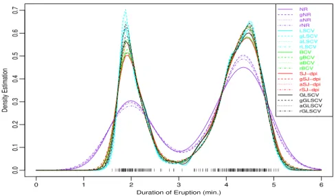
5. An Example

We realize an application for the all estimators with Gaussian kernel function. The application data is the durations (in minutes) of 272 eruptions of the Old Faithful geyser in Yellowstone National Park [9]. Fixed bandwidths for the kernel estimates are computed as ˆhN R = 0.394, ˆhLSCV = 0.103, ˆhBCV = 0.157,ˆhSJ = 0.165, and ˆhLSCV 4 = 0.128.

Figure 2 shows the data points and the considered all kernel estimates in this study. Figure 3 shows only the kernel estimates obtained based on selector GLSCV4.

All the estimates show clearly that the duration of eruption has a bimodal density. The adaptive kernel estimates behave similar to their classical kernel estimates tend to get better slightly. Specially, they lead to improve the estimates about the peaks and valley between the two peaks.

lll:••1ooo•~ •!t0

···.···

..

.

_.

_...

...

..

-·•

.

_..

_.

.

.

.

.

.

.

.

.

.

.

.

.

.

.

.

rn

..

..

.

-·..

.

..

.

.

..

.

.

.

..

....

..

....

.

_·

_.

_-.·

_•

·-...

···

:

·

·

.

t

••·

·

·

···

···

...

.

..

.

....

_.

_.

_{. .}

.

....

.... ····

_.

_·

_·

_···

_·

.

..

...

.

...

_·

_····

_·

_··

_··

_·

_·

·.

·

,

···

..

·,

•.

···

.

.

!

:

:!

::;!_

_.

_.

.

0 1 2 3 4 5 6 0.0 0.1 0.2 0.3 0.4 0.5 0.6 0.7

Duration of Eruption (min.)

Density Estimation | || | | | | | | | | | | | | | | | ||||||||||||||||||||||||||||||||||||||||||||||||||||||||||||||||||||||||||||||||||||| || || | |||||||||||||||||||||||||||||||||||||||||||||||||||||||||||||||||||||||||||||||||||||||||||||||||||||||||||||||||||||||||||||||||||||||||||||||||||||||||||||||||||| NR gNR aNR rNR LSCV gLSCV aLSCV rLSCV BCV gBCV aBCV rBCV SJ−dpi gSJ−dpi aSJ−dpi rSJ−dpi GLSCV gGLSCV aGLSCV rGLSCV

Figure 2. Classical and adaptive kernel density estimates.

1 2 3 4 5 6 0.0 0.1 0.2 0.3 0.4 0.5 0.6 0.7

Duration of Eruption (min.)

Density Estimation | ||| | | | | | | | | | | | | | | ||||||||||||||||||||||||||||||||||||||||||||||||||||||||||||||||||||||||||||||||||||| || || | |||||||||||||||||||||||||||||||||||||||||||||||||||||||||||||||||||||||||||||||||||||||||||||||||||||||||||||||||||||||||||||||||||||||||||||||||||||||||||||||||||| GLSCV gGLSCV aGLSCV rGLSCV

Figure 3. Adaptive kernel density estimates based on the bandwidth

selector LSCV4.

6. Conclusions

The adaptive kernel density estimators are often used for the estimation of densities far from normal distribution. The classical kernel density estimators are based on using the fixed bandwidths. The generalized LSCV estimator is a new efficient kernel density estimator which uses fixed bandwidth. It improves the finite sample behavior of the classical LSCV estimator.

The adaptive estimators use the different bandwidth for each observation point. There-fore, they are more robust to the existence of outliers or extremes. Here, we focused the adaptive variates of the generalized LSCV estimator. We also compared the perfor-mances of the other adaptive estimates. The results show that the adaptive estimators often significantly improves the classical estimators.

References

[1] Abramson, I.S. On bandwidth variation in kernel estimates-a square root law, Annals of Statistics 10, 1217–1223, 1982.

[2] Bowman, A. An alternative method of cross-validation for the smoothing of density

esti-mates, Biometrika 71, 353–360, 1984.

[3] Breiman, L., Meisel, W., and Purcell, E. Variable kernel estimates of multivariate densities, Technometrics 19, 135–144, 1977.

[4] Chiu, T. A comparative review of bandwidth selection for kernel density estimation, Statis-tica Sinica 6, 129–145, 1996.

[5] Core Team, R. R: a language and environment for statistical computing, R Foundation for Statistical Computing, Vienna, Austria, 2014.

[6] Cula, S., Demir, S., and Toktamis, O. The Finite Sample Performance of Modified Adaptive

Kernel Estimators for Probability Density Function, J Sci Res Rep, 11 (5), 1–9, 2016.

[7] Hall, P. and Marron, J.S. Variable window width kernel estimates of probability densities, Probability Theory and Related Fields, 80, 37–49, 1988.

[8] Hall, P. and Marron, J.S. Local minima in cross-validation functions, Journal of the Royal Statistical Society, Series B, 53, 245–252, 1991.

[9] Hardle, W. Smoothing Techniques with Implementation in S (Springer-Verlag, 1991). [10] Jones, M.C. Variable Kernel Density Estimation and Variable Kernel Density Estimation,

Australian Journal of Statistics, 32 (3), 361–371, 1990.

[11] Loader, C.R. Bandwidth selection: classical or plug-in, Annals of Statistics 27, 415–438, 1999.

[12] Park, B. U. and Marron J. S. Comparison of data-driven bandwidth selectors. Journal of the American Statistical Association, 85, 66–72, 1990.

[13] Scott, D. W. Multivariate Density Estimation (Wiley, 1992).

[14] Scott, D.W. and Terrell, G.R. Biased and unbiased cross-validation in density estimation, Journal of the American Statistical Association 82 (400), 1131–1146, 1987.

[15] Sheather, S.J. and Jones M.C. A reliable data-based bandwidth selection method for kernel

density estimation, Journal of the Royal Statistical Society Series B, 53, 683–690, 1991.

[16] Sheather, S.J. Density estimation, Statistical Science 19 (4), 588–597, 2004.

[17] Silverman, B. W. Density Estimation for Statistics and Data Analysis (Chapman&Hall, 1996).

[18] Terrell, G.R. and Scott, D.W. Variable kernel density estimation, Annals of Statistics 20 (3), 1236–1265, 1992.

[19] Van Kerm, P. Adaptive kernel density estimation, Stata Journal, 3, 148–156, 2003. [20] Wand, M. P. and Jones, M. C. Kernel Smoothing (Chapman&Hall, 1995).

[21] Zhang, J Adaptive normal reference bandwidth based on quantile for kernel density

estima-tion, Journal of Applied Statistics, 38 (12), 2869–2880, 2011.

[22] Zhang, J Generalized least squares cross-validation in kernel density estimation, Statistica Neerlandica, 69, 315–328, 2015.