Improved Position Estimation Using Hybrid
TW-TOA and TDOA in Cooperative Networks
Mohammad Reza Gholami, Student Member, IEEE, Sinan Gezici, Senior Member, IEEE, and
Erik G. Ström, Senior Member, IEEE
Abstract—This paper addresses the problem of positioning
mul-tiple target nodes in a cooperative wireless sensor network in the presence of unknown turn-around times. In this type of cooper-ative networks, two different reference sensors, namely, primary and secondary nodes, measure two-way time-of-arrival (TW-TOA) and time-difference-of-arrival (TDOA), respectively. Motivated by the role of secondary nodes, we extend the role of target nodes such that they can be considered as pseudo secondary nodes. By modeling turn-around times as nuisance parameters, we derive a maximum likelihood estimator (MLE) that poses a difficult global optimization problem due to its nonconvex objective function. To avoid drawbacks in solving the MLE, we linearize the measure-ments using two different techniques, namely, nonlinear processing and first-order Taylor series, and obtain linear models based on un-known parameters. The proposed linear estimator is implemented in three steps. In the first step, a coarse position estimate is obtained for each target node, and it is refined through steps two and three. To evaluate the performance of different methods, we derive the Cramér–Rao lower bound (CRLB). Simulation results show that the cooperation technique provides considerable improvements in positioning accuracy compared to the noncooperative scenario, es-pecially for low signal-to-noise-ratios.
Index Terms—Cooperative positioning, Cramér–Rao lower
bound (CRLB), linear estimator, maximum-likelihood esti-mator (MLE), time-of-arrival (TOA), time-difference-of-arrival (TDOA), two-way time-of-arrival (TW-TOA), wireless sensor network.
I. INTRODUCTION
N
OWADAYS wireless sensor networks (WSNs) have been considered for many civil and military applications. Position information is one of the critical requirements for a WSN that can be carried out by the network itself [1]–[3]. Most studies in the literature assume that there are a number of reference nodes, also called anchor nodes, that can be usedManuscript received April 04, 2011; revised December 27, 2011; accepted March 22, 2012. Date of publication April 13, 2012; date of current version June 12, 2012. The associate editor coordinating the review of this manuscript and approving it for publication was Prof. Philippe Ciblat. This work was sup-ported in part by the European Commission in the framework of the FP7 Net-work of Excellence in Wireless COMmunications NEWCOM++ (Contract no. 216715) and in part by the Swedish Research Council (Contract no. 2007-6363). This work was presented in part at the IEEE International Workshop on Signal Processing Advances for Wireless Communications, San Francisco, California, June 26–29, 2011.
M. R. Gholami and E. G. Ström are with the Division of Communication Sys-tems, Information Theory, and Antenna, Department of Signals and SysSys-tems, Chalmers University of Technology, SE-412 96 Göthenburg, Sweden (e-mail: [email protected]; [email protected]).
S. Gezici is with the Department of Electrical and Electronics Engineering, Bilkent University, Ankara 06800, Turkey (e-mail: [email protected]).
Color versions of one or more of the figures in this paper are available online at http://ieeexplore.ieee.org.
Digital Object Identifier 10.1109/TSP.2012.2194705
to estimate the position of an unknown target node [4]–[6]. In one viewpoint, positioning algorithms can be categorized based on measurement types such as time-of-arrival (TOA), time-difference-of-arrival (TDOA), received signal strength, and angle-of-arrival [1], [7].
Positioning algorithms based on TOA (or TDOA) need a chronized network [1] that can be handled using different syn-chronization techniques [8]–[12]. The process of synchronizing the sensor nodes is a cumbersome and costly task. Alternatively, two-way TOA (TW-TOA) has been considered as an effective approach in the literature (e.g., [13] and [14]) and has been stan-dardized [15], [16], mainly because of its relatively high accu-racy and lack of synchronization requirements. In this approach, a reference node sends a signal to a target node, and waits for a response from it. The round-trip delay time between the refer-ence node and the target node gives an estimate of the distance between them. As the number of reference nodes in a WSN in-creases, the position of the target node can be estimated more accurately via TW-TOA estimation.
Since, in practice, there are some limitations on increasing the number of reference nodes due to power and complexity con-straints, the idea of cooperation between reference nodes was proposed in [17] to decrease the number of transmissions, and its theoretical analysis was presented in [14]. In this method, some reference nodes, called primary reference nodes (PRNs), initiate range estimation by sending a signal. The target node replies to received signals by sending an acknowledgement after a processing delay called the turn-around time. It is assumed that there are some other reference nodes, which can listen to both signals, and these are called as the secondary reference nodes (SRNs). It has been shown that SRNs can help PRNs es-timate the target node position more accurately [14]. In fact, it is possible to get the same performance with fewer PRNs when measurements from SRNs are involved in the positioning process. It is assumed that SRNs are able to receive signals from both a target node and PRNs [14]; therefore, SRNs are able to measure the TDOA between the target node’s signal and the sig-nals of the PRNs. Indeed a hybrid set of TW-TOA and TDOA measurements is available to estimate the position of a target node. Positioning of a single target using cooperative primary and secondary sensors is studied in [14], [18], and [19]. In the previous studies, it was assumed that either an estimate of the turn-around time is available [14] or it is extremely small such that it can be neglected [18], [19]. The model considered in this study is based on cooperation between primary and secondary reference nodes, which is different from targets cooperation in traditional cooperative networks [20]. It should also be noted that the idea of employing listening nodes was previously con-sidered in bistatic radars in a different context [21].
In this paper, we consider target nodes as ordinary sensors that can measure the TOA of the received signals. Motivated by the role of the secondary nodes, we extend the model of a single target node positioning to multiple target nodes positioning where for every target node the remaining target nodes play the role of pseudo secondary nodes with unknown positions. We further assume that no a priori knowledge of the turn-around time is available and it is modeled as a deterministic unknown parameter. To derive different algorithms for position estima-tion in cooperative networks, we model the turn-around times at different targets as nuisance parameters that can be jointly estimated with targets’ positions. Moreover, assuming known probability distribution for TOA errors as Gaussian random variables, we derive a maximum-likelihood estimator (MLE) to solve the positioning problem. However, the MLE poses a diffi-cult global optimization problem due to the nonconvex nature of its objective function. Therefore, we need to resort to numerical methods, e.g., an iterative search algorithm with a good initial point. Generally, in the positioning literature, to cope with dif-ficulty in solving an MLE, different techniques such as convex relaxation techniques, e.g., semidefinite and second order cone programming [22]–[27], set theoretic approach [28]–[32], and linearization techniques [33]–[36] are employed.
In this current work, in order to avoid drawbacks in solving the MLE, we employ linearization techniques to obtain a linear estimator for the positioning problem considered in this study. The linear estimator that we obtain is implemented in three steps: In the first step, assuming small variances of measurement errors and using a nonlinear pre-processing on measurements, a linear model based on target node’s position and turn-around time is obtained. The linear (weighted) least squares method is employed to solve the problem. Since the linear estimator is a suboptimal estimator for the positioning problem [37], a number of techniques such as correction techniques can be used to im-prove the performance of the estimator [33], [36]. We employ a modified correction technique, inspired by the work in [35], to enhance the performance of the linear estimator. Note that in the first step, a coarse position estimate is obtained for every target node. In the second step, considering measurements between target nodes and using the first step estimation, the turn-around time is estimated using a simple linear estimator. And finally, in the third step, using the first-order Taylor series expansion, a new linear model is obtained and then we apply a regulariza-tion technique, namely, the Tikhonov regularizaregulariza-tion approach [38], to solve the problem. Note that the step one and step two of the linear estimator can be locally performed in target nodes while the step three of the linear estimator and the MLE need centralized processing. Moreover, to evaluate the performance of different methods, we derive the Cramér–Rao lower bound (CRLB) for this problem. Simulation results confirm that for sufficiently large signal-to-noise-ratios (SNRs), the proposed estimator can get very close to the CRLB.
Note that the measurement errors can be non-Gaussian, e.g., in non-line-of-sight (NLOS) scenarios. However, we con-sider the Gaussian assumption in this study for the following purposes:
1) closed-form expressions can be obtained for the theoret-ical limits and the proposed estimator under the Gaussian model;
2) the cooperative positioning scenario studied in this man-uscript has not been investigated before in the literature, even for Gaussian error models; therefore, this study can be considered as a first step in the investigation of such scenarios, and non-Gaussian error models can be consid-ered as future studies;
3) the model/estimators studied in this paper can be extended to cover NLOS scenarios if the errors can be modeled as Gaussian random variables with positive means [39]. In summary, the main contributions of this study are as follows:
1) a new model for multiple target nodes positioning in coop-erative networks in which for every target node the other target nodes play the role of pseudo secondary nodes; 2) a joint turn-around time and position estimation idea for
the TW-TOA;
3) derivation of the MLE and the CRLB for the cooperative networks considered in this study;
4) a novel three step linear estimator based on linearizing the measurements using two different techniques: nonlinear processing and first-order Taylor series.
The remainder of the paper is organized as follows. Section II explains the system model and the problem formulation con-sidered in this paper. The optimal estimator and theoretical limits are derived in Section III. In Section IV, a three-step linear estimator is obtained. Simulation results are discussed in Section VI. Finally, Section VII makes some concluding remarks.
Notation: The following notations are used in this paper.
lowercase Latin/Greek letters, e.g., , denote scalar values and bold lowercase Latin/Greek letters show vectors. Matrices are shown by bold uppercase Latin/Greek letters. and de-note the vector of ones and the vector (matrix) of all zeros, respectively. is the by identity matrix. The operators and are used to denote the trace of a square matrix and the expectation of a random variable (or vector), respec-tively. The Euclidian norm of a vector is denoted by . For a matrix , the Frobenius norm of , i.e., , is
de-fined as . The
is a (block) diagonal matrix with diagonal elements (blocks) and shows the cardinality of the set . de-notes the ceiling function and is the Euclidian norm of , i.e., . The function denotes the modulo operation that gives the remainder of division of by .
II. SYSTEMMODEL ANDPROBLEMSTATEMENT
Let us consider a two-dimensional network1with
sensor nodes. Suppose that the first reference nodes
are located at known positions ,
and the remaining target nodes are placed at
unknown positions ,
. For simplicity, we assume that the first sensors are the PRNs and the next sensors are the SRNs. Sup-pose that the PRNs are used to measure the TW-TOA between the PRNs and the target nodes and that SRNs are able to listen and measure signals transmitted by both the PRNs and the target nodes.
1The generalization to a three-dimensional scenario is straightforward, but is
Let us define , , and
as the set of indices of primary, secondary, and
target nodes, respectively. Let PRN
can communicate with target node and SRN can receive both signals transmitted by PRN and target node as the set of all pairs with one primary node and one secondary node that are connected to each other and also connected to target node . We also define
PRN can communicate with target node
and target node can receive
both signals transmitted by PRN and target node as the set of all pairs with one primary node and one target node that are connected to each other and also connected to target node . For notational convenience, let us order the elements of
sets and , and write and ,
where
(1) To simplify later calculations, we further assume that the SRNs and targets connected to target are connected to the same set of primary nodes, i.e.,
(2) The TW-TOA measurement between primary node and target node can be written as [14]
(3) where is the speed of propagation, is the Euclidian distance between PRN and the point , is the turn-around time in response to the signal transmitted by the th PRN at target node is the TOA estimation error at target node for the signal transmitted by the th PRN, and is the TOA estimation error at the th PRN for the signal received from target node . The estimation errors are modeled as zero mean Gaussian random variables with variances and ; i.e.,
and [6], [14].
Suppose that SRNs and other target nodes are able to measure the TOA of the received signal from target node and PRN connected to target node . The TOA estimates of the signal received from the th PRN, during the TW-TOA measurement with target node , at SRN and at target node are
(4a) (4b) where the th PRN sends its signal at time instant to target node , which is unknown to SRN and to target node ,
and are the distances between PRN to SRN and to target node , respectively, and are modeled as zero mean Gaussian random variables with
variances and , i.e., and
.
Suppose that the response signal from target node to this signal is also received at SRN and at target node as well. The TOA estimates for these signals at SRN and at target node are given by
(5a)
(5b) Having two measurements in SRN , namely, measurements in (4a) and in (5a), we are able to measure the TDOA between PRN and target node corresponding to the distance from PRN to target node plus two additional distances; distance from target node to SRN and a distance due to the unknown turn-around time, i.e., , at target node .
To gain some insight into the problem, let us consider Fig. 1 and Fig. 2, where one PRN (PRN 1) performs the TW-TOA es-timation with Target 4. Namely, PRN 1 sends a signal to Target 4 at time instant , and Target 4 replies to this signal after , see Fig. 2. Suppose that three other nodes, SRN 2, SRN 3, and Target 5, listen to both signals. Since the distances between the reference nodes are known, it is possible in the secondary node to estimate the time reference from (4a), e.g., SRN 2 in Fig. 2; Hence, SRNs are able to estimate the overall distance from PRN to target node and target node to SRN plus the additional distance due to the delay , assuming that is positive, as follows:
(6) where is an estimate of at the th SRN, e.g.,
, , , and
.
Similar to the process for the SRNs, other target nodes that receive both signals from PRN and target node can play the role of secondary nodes, e.g., Target 5 in Figs. 1 and 2. Sub-tracting (5b) from (4b) and then multiplying with yields
(7)
where and .
In (6), parameters of target node , i.e., and , are un-known, while in (7) besides the parameters of target node , the position of unknown target node , i.e., , is also present. Note that target node cannot make an estimate of since the distance between PRN and target node is known in ad-vance. From (3), the distance estimate to target node in the th
Fig. 1. A cooperative network consisting of one primary node, three secondary nodes, and two target nodes. Here the primary node initiates the TW-TOA mea-surement with Target 4. Both signals transmitted by PRN 1 and Target 4 are received at SRN 2, SNR 3, and Target 5.
Fig. 2. The primary node 1 transmits a signal at and Target 4 responses to the received signal after . SNR 2 and Target 5 receive both signals trans-mitted by PRN 1 and Target 4, and compute TDOA measurement.
PRNplus additional distance due to the unknown turn-around time is expressed as
(8)
where and . Let us define the vector of
measurement as
(9) where
(10)
The goal of a positioning algorithm is to find the position of target nodes based on the position of the known sensor nodes and measurements made in (9).
In the positioning literature, it is commonly assumed that ei-ther an estimate of is available [14], or it is extremely small
such that it can be neglected [18], [19]. Since the estimation of the turn-around time needs an accurate calibration, it may gener-ally increase the complexity. In this paper, we assume that no a
priori knowledge of the turn-around time is available. Since the turn-around time depends on the processing time at a target node, it is then reasonable to assume a constant value for it. Here we assume that for every target node, the turn-around time is
un-known but fixed for all links, i.e., .
III. OPTIMALESTIMATOR ANDTHEORETICALLIMITS
In this section, we first derive the MLE for the positioning problem and in the sequel a theoretical lower bound on the vari-ance of any unbiased estimator is obtained. To derive the MLE, we consider turn-around times as nuisance parameters that can be estimated along with target nodes’ positions.
A. Maximum Likelihood Estimator
To find the MLE, we need to find the probability distribu-tion funcdistribu-tion (PDF) of the measurement vector in (9). In Appendix A, the PDF of measurement vector , i.e., , is computed. The MLE then can be obtained by the following optimization problem:
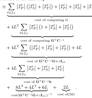
(11) where is defined in (58). The expression for the MLE is given by (12) at the bottom of the next page, where , , , and
are given in Appendix A, i.e., (60) and (64).
As can be seen, the MLE forces a difficult global optimization problem due to nonlinearity and nonconvexity issues. There-fore, we need to resort to the numerical methods, e.g., an itera-tive search algorithm with a good initial point. To avoid draw-backs in solving the MLE, in the next section we derive a three-step linear estimator that approaches the CRLB for sufficiently high SNRs.
Note that for a single target node and a known turn-around time, expression in (12) changes to the MLE derived in [14]. It
is also observed that when and , i.e., a
noncooperative scenario (conventional network) where , the MLE reduces to the well-known weighted nonlinear least squares estimator
(13)
B. Cramér–Rao Lower Bound
Since the TOA errors are Gaussian random variables, in (9) is modeled as a Gaussian random vector with mean and covariance matrix , i.e., , where mean vector and covariance matrix are as computed in Appendix B.
Considering the measurement vector in (9) with mean and covariance matrix , which are given by (65) and (67), respec-tively, the Fisher information matrix can be computed as [40]
where
if if if
(14) Based on (66), can be obtained as follows:
(15)
where [see (16)–(18), shown at the bottom of the page]. The CRLB, which is a lower bound on the variance of any unbiased estimator, can be obtained as
(19)
For the single target node, the CRLB in (19) reduces to
(20) (12) if if if otherwise (16) if if if otherwise (17) if if if if if otherwise (18)
where and is a lower bound on the variance of any unbiased estimator when the perfect knowledge of the turn-around time is available [14]. For the perfect knowledge of the turn-around time, i.e., ,
, 2, 3, (20) tends to .
Note that all results obtained here and in the previous section can also be applied to conventional networks in which there are only primary nodes.
IV. LINEARESTIMATOR
In this section, using linearization techniques, we obtain a linear estimator to solve the positioning problem for cooperative networks. In the proposed estimator, we first obtain a coarse estimate for the position of the target nodes, and then refine them in the next steps.
A. First Step
One way to obtain a linear model versus the target node’s position is to apply a nonlinear pre-processing on measurements [34], [41], [42]. Suppose that the level of noise is small. Let us move the term , recalling that , in (8) to the left-hand-side. Now squaring both sides, after dropping the small term, yields
(21) where . A linear model can be obtained as follows:
(22)
where .
For the TDOA measurement at the th SRN, i.e., (6), we first arrange a new set of measurements as
(23)
where . Now similar to (21),
we can linearize (23) to get
(24) Again a linear model based on unknown parameters is obtained as follows:
The linear set of equations can be written as
(25) where (26a) .. . ... ... .. . ... ... (26b) (26c) Using the least squares criterion [40, Ch. 8], a closed-form solution to (25) can be obtained as
. If matrix is
ill-conditioned, we can use the regularization technique [38, Ch. 6] to get
(27) where parameter defines the tradeoff between
and , and the covariance matrix of the zero mean noise vector is as computed in Appendix C.
We here show for a large network, matrix in (26b) is ill-conditioned, i.e., has a large condition number (CN). To that aim, we first find a lower bound on the CN of the matrix .
Lemma 4.1: Let be an by matrix with ordered singular values . Let denote a submatrix of derived by deleting a total of rows/or columns from . Suppose the ordered singular values of are . Then
(28)
where for a by matrix we set if .
Proof: Please see [43, Ch. 3, Corollary 3.1.3].
Proposition (Sufficient condition): Let , where , be a submatrix of the in (26b) derived by deleting the last column (the 4th column) of matrix . If (e.g., this is the case for a large network where some entries of matrix have large values), then the CN of matrix is large and the matrix is ill-conditioned.
Proof: Suppose that matrix has full column-rank, i.e., , where is the number of rows of matrix and , , 2, 3, 4, are column vectors, e.g.,
. Let be the singular values of
Therefore, a lower bound on the largest of the matrix , although not very tight, can be found as
(29) Now we find a simple upper bound on the smallest singular value . Suppose that we delete all the columns except the column 4. Then, using Lemma 4.1, we can write
(30) According to (29) and (30), a lower bound on the CN of the matrix in (26b) can be obtained as
CN of matrix (31)
Although the lower-bound in (31) is not very tight, it is suf-ficient to show that, for large networks, when matrix has
, then it is ill-conditioned. In fact,
This condition is sufficient and it does not claim that if the en-tries of the matrix are small, the CN is consequently small.
Similar matrices have appeared in the positioning litera-ture when the least squares approach is employed to solve the problem, e.g., see [33]–[36] and [45]. Therefore, if large networks are considered, those matrices are ill-conditioned.
Let us decompose the positive semidefinite matrix using singular value decomposition as
where and are orthogonal and diagonal matrices, respec-tively. Considering , we can compute the bias of the estimator as
(32) where . It is observed that the estimator in (27) is biased in general. However, it can be shown that for high SNRs, the estimator tends to be an unbiased estimator. The covariance matrix of can be computed as
(33) To compute the covariance matrix , the real distances be-tween reference nodes to the target is required. Since, in prac-tice, the real distances are not available, we instead use the es-timated distances. To do this, first we can compute (27) by re-placing with the identity matrix, and then we can obtain the distance estimate from reference nodes to the target. It has been shown in [41] that the degradation of replacing the estimated distances instead of the real distances is negligible.
Since the elements of estimated parameters in (27) are de-pendent, one method to improve the estimation accuracy, called
the correction technique [33], [35], [36], is to take this relation between elements of into account. Here, we extend the cor-rection technique to our problem. Suppose each element of (27) can be written as
(34)
where is the error of estimation .
Let the errors on estimation be considerably small. Therefore, squaring both sides of the first three elements of (34) yields
(35) Hence, the relation between the estimated elements in (27) can be written, using (35), as
(36) where
(37)
The least squares approximation of is obtained from (36) as
(38) where covariance matrix can be computed as
(39)
where .
To compute the covariance matrix , since the exact value of the unknown vector is not available, the estimated one from (27) is replaced. The covariance matrix of is given by
(40) Finally, the target position can be obtained as follows:
(41) The estimate obtained in (41) is a coarse estimate and it is refined in step three.
The covariance matrix of the estimator in (41) can be com-puted similar to [35] as follows. Suppose that the estimate in (38) can be written as
(42) where is the error of estimation in (38). Using the first-order Taylor-series expression, assuming small error , we get
(43) Hence, the covariance matrix of can be computed as
(44)
where and
de-notes the upper left part of matrix .
B. Second Step
In this step, we consider the measurements taken in (7) be-tween target nodes that were not involved in the first step. Since the turn-around time is linearly dependent on the measurements in (7), we derive a simple estimator for the turn-around time es-timation.
For a small error of estimation, let us apply the first-order Taylor-series expansion for the measurements in (7) about (41)
(considering , ) as follows:
(45) If the distribution of random vector is known, it is possible to derive the MLE for the turn-around time . For high SNRs, the estimator obtained in the last section is approximately an unbiased estimator, i.e., , . Instead of deriving the MLE, an estimator based on the least squares criterion can be obtained, and we can estimate the turn-around time as
(46)
A more accurate estimation can be obtained considering the weighting matrix based on the covariance matrix of the noise. We leave it here since the simple averaging estimator works well as we observed through simulations.
C. Third Step
In the final step, the estimate of target nodes’ positions is re-fined. The difference between this step and two previous steps is that here all target nodes’ positions are corrected simultaneously while in the two last steps, every estimation parameter, i.e., the position of the target node or the turn-around time, is updated one by one. Based on the estimation in the step one and two, namely estimation in (41) and (46), let us apply the first-order Taylor series expansion to whole measurements. For target node
, we get
(47a)
(47b)
(47c) Therefore, from (47a), (47b), and (47c) a new linear model based on the error of estimation can be derived as
(48)
where and
, and vector is obtained as
follows:
(49) where
(50) Let matrix be written as
(51) where submatrix is obtained as
and vectors , , and are obtained as if if if . (53) To solve (48), we note that the new linear model is derived as-suming small errors of estimation. Hence, to obtain the estima-tion error from (48), i.e., , to be small enough (if possible), we solve a regularized least squares problem as follows:
(54) where the regularization parameter determines the
tradeoff between and , and
stands for the weighted norm . The solution to (54), Tikhonov regularization problem, is given by [38, Ch. 6]
(55) where the covariance matrix is given by (67) in Appendix B. Finally, the updated estimate in this step is
(56) It is noticed that step three can be repeated for a number of updates; however, as observed in the simulations, one round of update is sufficient to get very close to the CRLB. Note that similar procedures can be derived for the conventional networks.
V. COMPLEXITYANALYSIS
In this section we evaluate the complexity of the estima-tors considered in this study based on the total number of the floating-point operations or flops. We assume that an addition, subtraction, multiplication, division, or square root operation in the real domain can be computed by one flop. We calculate the total number of the flops for every method and express it as a polynomial of the free parameters [46]. To simplify the expres-sion, we keep only the leading term of the complexity expression.
A. The Maximum Likelihood Estimator
As previously mentioned, the MLE is nonlinear and non-convex. The complexity of the MLE highly depends on the solution method. Moreover, for every method we may have a number of parameters that affect the complexity, e.g., the number of iterations, the initial point, or the solution accuracy. We leave the complexity analysis of methods that may be used to solve the MLE and instead we compute the cost of evaluating the objective function of the MLE (12) for a certain point. To do that we first compute the cost of each element in
(12) separately. We need six flops to compute a distance. For
computing , , and , we require 9,
15, and 22 flops, respectively (we consider as a single
variable). Similarly, needs flops to
compute. Then the total number of flops for evaluating the MLE at a point can be computed as
MLE flops
Therefore, for dense networks the leading term is MLE flops
B. The Linear Estimator
For the linear estimator, we compute the complexity for each step. Hence, the total cost is the sum of the complexity of three steps. There are a number of ways to find the complexity of a linear estimator, e.g., see [47], [48]. Here, we derive the plexity for the worst case without any attempt to optimize com-putations to take advantage of, e.g., the structure of matrices.
1) First Step: We first compute the complexity of computing
. can be computed by flops.
Now we compute the positive definite matrix by
flops. The
ma-trix multiplication requires flops.
Therefore, the total complexity of (27) can be computed as: First step flops
Similarly, we can find the complexity of the correction tech-nique. It can be verified that the complexity of the correction technique is negligible compared to the cost of (27) since the most complex part, i.e., (33), has been already computed. Then, for every target we can define the complexity by getting the leading term as
First step flops
The total cost for all targets can be computed as Total cost of the first step
TABLE I
COST OFDIFFERENTAPPROACHES FOR AFULLYCONNECTEDNETWORK, , , and
2) Second Step: The cost of the turn-around time estimation
for target node can be computed as Second step flops
Then considering the leading terms, the total cost for all targets can be computed as
Total cost of the second step
3) Third Step: From the first step, we can compute the matrix
with a little modification. Hence, when computing the overall cost for an algorithm that involves both step one and three, we can disregard the cost for computing when formu-lating the cost for step three. We will follow this approach here, and the complexity of the estimation in (55), remembering block diagonal nature of the matrix , can be computed as follows:
Total cost of the third step
Table I shows the cost of different approaches (considering the leading terms) for a fully connected network.
VI. SIMULATIONSRESULTS
In this section, computer simulations are performed to evaluate the performance of the different approaches. To com-pare different methods, we consider the root-mean-square-error (RMSE) for target node defined as
(57) The network deployment shown in Fig. 3(a) consists of four PRNs (sensor nodes 1, 2, 3, and 4), four SNRs (sensor nodes 5, 6, 7, and 8), and six targets (sensor nodes 9, 10, 11, 12, 13, and 14). The connectivity matrix for the network is shown in Fig. 3(b), where every target is connected to a number of PRNs, SRNs, and other targets. For instance target node 9 is connected
to primary nodes 1, 2, and 4, to secondary nodes 5 and 8, and to targets 10, 11, 13, and 14. In every realization for a target node, the turn-around time is randomly drawn from [10, 1000] ns. We
also assume that . In all simulations,
joint estimation of the turn-around time and the position is con-sidered unless stated otherwise. In addition, no attempt is taken to choose the optimum value for the regularization parameters
and we simply set and . To compute the
MLE, we employ Matlab’s function lsqnonlin [49] initialized with the true values of the positions and turn-around times of targets. In the simulations, we consider targets 9, 12, 13, and 14.
A. Effects of the Turn-Around Time
In this section, we study the effects of involving turn-around times in the estimation process for different scenarios. In the conventional network (Conv.), the measurements in PRNs are used to jointly estimate the position of a target and its turn-around time. For the cooperative network, we distinguish be-tween involving only SRNs (Coop. 1) and involving both SRNs and target nodes (Coop. 2) in the estimation process.
In Fig. 4, we illustrate the CRLBs of position estimation for different networks. For every network, the CRLB is plotted for two cases; the perfect knowledge of the turn-around time and the joint estimation of the turn-around time and the position. It is observed that estimating the turn-around time as a nuisance pa-rameter can deteriorate the accuracy of the position estimation. For target nodes 9 and 12, the difference between two cases is negligible, while there is a more noticeable difference for target nodes 13 and 14, especially for target node 14. For target node 14 for the conventional network, the gap between the two curves increases as the standard deviation of noise increases while for the cooperative networks (Coop. 1 and Coop. 2) the CRLB of the joint estimation of the turn-around time and the target posi-tion is very close to the CRLB of the case in which the perfect knowledge of the turn-around time is available. It is clear from the figure that the cooperation idea improves the performance of the estimator especially for high values of the standard de-viation of noise. It is concluded that involving target nodes as pseudo secondary nodes improves the performance as well.
For further investigations, we study the case when the par-tial knowledge of the turn-around time is available. This in-formation can be obtained by, for instance, calibrating a target node with a fixed sensor node. The target node can estimate its turn-around time using loopback test and then transmit it to other sensor nodes [13], [14]. Let us model the turn-around time of target node as a Gaussian random variable with mean
and variance , i.e., .
Fig. 5 shows the CRLBs of target node 9 and 14 in various scenarios when partial knowledge of the turn-around time is available in different sensor nodes. We fix the standard
devi-Fig. 3. (a) The network deployment used in the simulation (b) The connectivity matrix: the x-marker shows which nodes are connected.
Fig. 4. CRLBs of different networks for different targets: (a) target 9; (b) target 12; (c) target 13; and (d) target 14.
ation of the TOA estimation error to be equal to 10 and 30 m and plot the CRLB versus standard deviation . It is again observed that the cooperative networks outperform the conventional network. Based on Fig. 4 and Fig. 5, we can obtain a benchmark to specify the values of and for which the joint estimation of position and turn-around time outperforms to the case in which the partial knowledge of the turn-around time is available. For instance for target 14, Coop. 1 for 30 m
has better performance compared to the case in which partial knowledge of the turn-around time with is available.
B. Performance of Estimators
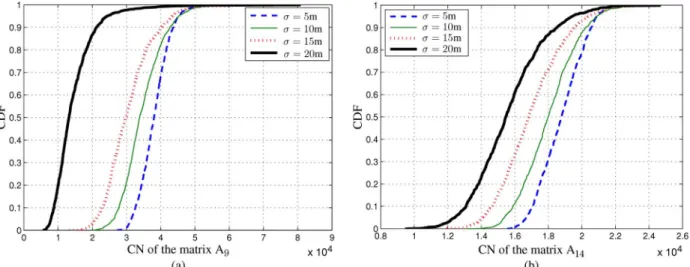
As mentioned in Section IV-A, matrix in (26b) has a large CN if a large network is considered. For the network consid-ered in the simulations, we plot the cumulative distribution func-tion (CDF) of the CN of matrix for target 9 and 14 in Fig. 6
Fig. 5. CRLBs of different networks for different targets: (a) target 9 and (b) target 14.
Fig. 6. CDF of CN of the matrix for different values of : (a) target node 9 and (b) target node 14.
Fig. 7. RMSE of CRLB, MLE, and linear estimator for the cooperative network (Coop. 2) for (a) target node 9 and (b) target node 14.
for 3000 realizations of noise for different values of . It can be observed that the CN of matrix is large; hence, the regular-ization technique is one option in order to solve the linear model in (25).
Fig. 7 shows the RMSEs of the MLE, the CLRB, and the linear estimator for the cooperative network (Coop.2) for target
nodes 9 and 14. It is observed that the linear estimator in step three attains the CRLB for sufficiently high SNRs. It is also seen that removing step two and considering a two step linear esti-mator, i.e., a linear estimator consisting of step one and step three, deteriorates the performance for low (high SNR). For high SNRs, it seems that the estimation of the turn-around time
in the first step is more accurate than the one in the second step. Then, the estimation of the target position in step three can be af-fected by the accuracy of the turn-around time estimation. Note that we do not attempt to obtain the optimum regularization pa-rameters in the simulations.
VII. CONCLUSION
In this paper, we have studied the multi-target positioning problem in cooperative sensor networks using TW-TOA and TDOA measurements performed by primary and secondary nodes, respectively. We have assumed that there is no a priori knowledge of the turn-around time at target nodes and we have modeled them as nuisance parameters that can be jointly estimated with the position of the targets. We have proposed a new model for multiple target nodes positioning where target nodes can play the role of secondary nodes. Then, we have derived an MLE that forces a difficult global optimization problem due to the nonconvex nature of its cost function. To cope with the difficulty in solving the MLE, we have used two different linearization techniques to obtain linear estimators. The proposed estimator is implemented in three steps: In the first step, a coarse estimate is obtained; and in the second and third steps, the estimates are refined. The advantage of the pro-posed linear estimator is that it can get very close to the CRLB for sufficiently high SNRs. For future studies, we can focus on situations in which some target nodes are just connected to a number of other target nodes. One approach for this scenario is to consider the TW-TOA measurements between the targets. Moreover, positioning in NLOS scenarios and designing robust algorithms, e.g., based on a projection approach, are of great interest for future studies. Finally, the effects of non-Gaussian measurement errors on the proposed linear estimator can be investigated based on practical TOA measurements.
APPENDIXA PDFOFMEASUREMENTS
Since measurements in (10) are correlated, due to the term in (6), (7), and (8), we first perform conditioning on
correlated terms, i.e., and then compute
, where
(58) In (58), is an unknown vector of positions and turn-around times of target nodes. From (8), (6), and (7) for given , we can write
(59)
where and
(60) The PDF of the noise vector can be computed as (due to independent samples)
(61) where . Having the conditional PDF (59) and the PDF of the noise vector , i.e., (61), we can obtain the PDF of the vector as follows:
(62)
where .
Using
for , the PDF of the measurements can be computed as:
where
(64)
APPENDIXB
MEANVECTOR ANDCOVARIANCEMATRIX OFMEASUREMENTS
The mean can be computed as
(65) where
(66a)
(66b)
Suppose that the covariance matrix is expressed as
..
. ... ... ... (67) It can then be shown that for . To compute , first consider the following expressions:
(68a) (68b) (68c) .. . . .. ... .. . . .. ... .. . ... . .. ... ... ... . .. ... .. . ... . .. ... ... ... . .. ... (72)
The matrix can be written as
(69)
where matrices ,
, and
are obtained as follows, assuming
(70) (71) with (72), shown at the bottom of the previous page.
APPENDIXC
COVARIANCEMATRIX IN THEFIRSTSTEPESTIMATION
Let us express the covariance matrix of zero mean random vector in (26c) as
(73)
where matrices ,
, and are given by
(74a) .. . ... ... ... (74b) .. . ... (74c) ACKNOWLEDGMENT
The authors would like to thank Prof. S. Kay and Prof. M. Viberg for comments on the linear estimator. They also would like to thank Dr. M. Rydström for the comments on the paper. The simulations were performed on resources provided by the Swedish National Infrastructure for Computing (SNIC) at C3SE.
REFERENCES
[1] G. Mao and B. Fidan, Localization Algorithms and Strategies for Wire-less Sensor Networks. New York: Hershey, 2009, Information Sci-ence referSci-ence.
[2] R. L. Moses, D. Krishnamurthy, and R. M. Patterson, “A self-localiza-tion method for wireless sensor networks,” EURASIP J. Adv. Signal Process., no. 4, pp. 348–358, Mar. 2003.
[3] N. Bulusu, J. Heidemann, and D. Estrin, “GPS-less low-cost outdoor localization for very small devices,” IEEE Pers. Commun., vol. 7, no. 5, pp. 28–34, Oct. 2000.
[4] A. H. Sayed, A. Tarighat, and N. Khajehnouri, “Network-based wire-less location: Challenges faced in developing techniques for accurate wireless location information,” IEEE Signal Process. Mag., vol. 22, no. 4, pp. 24–40, July 2005.
[5] S. Gezici, “A survey on wireless position estimation,” Wireless Pers. Commun. (Special Issue on Towards Global and Seamless Personal Navigation), vol. 44, no. 3, pp. 263–282, Feb. 2008.
[6] N. Patwari, J. Ash, S. Kyperountas, A. O. Hero, and N. C. Correal, “Locating the nodes: cooperative localization in wireless sensor net-work,” IEEE Signal Process. Mag., vol. 22, no. 4, pp. 54–69, Jul. 2005. [7] M. R. Gholami, “Positioning Algorithms for Wireless Sensor Networks” Licentiate thesis, Chalmers Univ. of Technol., Göte-berg, Sweden, Mar. 2011 [Online]. Available: http://publica-tions.lib.chalmers.se/records/fulltext/138669.pdf
[8] I. Sari, E. Serpedin, K. Noh, Q. Chaudhari, and B. Suter, “On the joint synchronization of clock offset and skew in RBS-protocol,” IEEE Trans. Commun., vol. 56, no. 5, pp. 700–703, May 2008.
[9] Q. M. Chaudhari, E. Serpedin, and K. Qaraqe, “Some improved and generalized estimation schemes for clock synchronization of listening nodes in wireless sensor networks,” IEEE Trans. Commun., vol. 58, no. 1, pp. 63–67, Jan. 2010.
[10] J. Zheng and Y. Wu, “Joint time synchronization and localization of an unknown node in wireless sensor networks,” IEEE Trans. Signal Process., vol. 58, no. 3, pp. 1309–1320, Mar. 2010.
[11] N. Khajehnouri and A. H. Sayed, “A distributed broadcasting time-synchronization scheme for wireless sensor networks,” in Proc. IEEE Int. Conf. Acoust., Speech, Signal Process., Mar. 2005, vol. 5, pp. v/1053–v/1056.
[12] Q. Chaudhari, E. Serpedin, and J. Kim, “Energy-efficient estimation of clock offset for inactive nodes in wireless sensor network,” IEEE Trans. Inf. Theory, vol. 56, no. 1, pp. 582–596, Jan. 2010.
[13] Z. Sahinoglu, “Improving range accuracy of IEEE 802.15.4a radios in the presence of clock frequency offsets,” IEEE Commun. Lett., vol. 15, no. 2, pp. 244–246, Feb. 2011.
[14] S. Gezici and Z. Sahinoglu, “Enhanced position estimation via node cooperation,” presented at the IEEE Int. Conf. Commun. (ICC), Cape Town, South Africa, May 23–27, 2010.
[15] Part 15.4: Wireless Medium Access Control (MAC) and Physical Layer (PHY) Specifications for Low-Rate Wireless Personal Area Networks (LRWPANs), IEEE P802.15.4a/D4 (Amendment of IEEE Std 802.15.4), Jul. 2006.
[16] Information Technology—Real-Time Locating Systems (RTLS)—Part 5: Chirp Spread Spectrum (CSS) at 2,4 GHz Air Interface, ISO/IEC ISO/IEC 24730-5, 2010.
[17] R. Fujiwara, K. Mizugaki, T. Nakagawa, D. Maeda, and M. Miyazaki, “TOA/TDOA hybrid relative positioning system using UWB-IR,” in IEEE Radio Wireless Week, Jan. 2009, pp. 679–682.
[18] M. R. Gholami, S. Gezici, M. Rydström, and E. G. Ström, “A dis-tributed positioning algorithm for cooperative active and passive sensors,” in Proc. 21st Annu. IEEE Int. Symp. Pers., Indoor, Mobile Radio Commun. (PIMRC), Istanbul, Turkey, Sep. 26–29, 2010, pp. 1711–1716.
[19] M. R. Gholami, S. Gezici, E. G. Ström, and M. Rydström, “Hybrid TW-TOA/TDOA positioning algorithms for cooperative wireless networks,” presented at the IEEE Int. Conf. Commun. (ICC), Kyoto, Japan, Jun. 2011.
[20] H. Wymeersch, J. Lien, and M. Z. Win, “Cooperative localization in wireless networks,” Proc. IEEE, vol. 97, no. 2, pp. 427–450, Feb. 2009. [21] B. Rigling, Advances in Bistatic Radar. Raleigh, NC: Scitech, 2007. [22] P. Biswas, T.-C. Lian, T.-C. Wang, and Y. Ye, “Semidefinite program-ming based algorithms for sensor network localization,” ACM Trans. Sens. Netw., vol. 2, no. 2, pp. 188–220, 2006.
[23] S. Srirangarajan, A. Tewfik, and Z.-Q. Luo, “Distributed sensor network localization using SOCP relaxation,” IEEE Trans. Wireless Commun., vol. 7, no. 12, pp. 4886–4895, Dec. 2008.
[24] P. Tseng, “Second-order cone programming relaxation of sensor net-work localization,” SIAM J. Optim., vol. 18, no. 1, pp. 156–185, Feb. 2007.
[25] J. Nie, “Sum of squares method for sensor network localization,” Comput. Optim. Appl., vol. 43, pp. 151–179, 2009.
[26] A. Beck, P. Stoica, and J. Li, “Exact and approximate solutions of source localization problems,” IEEE Trans. Signal Process., vol. 56, no. 5, pp. 1770–1778, May 2008.
[27] Z. Wang, S. Zheng, Y. Ye, and S. Boyd, “Further relaxations of the semidefinite programming approach to sensor network localization,” SIAM J. Optim., vol. 19, pp. 655–673, Jul. 2008.
[28] D. Blatt and A. O. Hero, “Energy-based sensor network source local-ization via projection onto convex sets,” IEEE Trans. Signal Process., vol. 54, no. 9, pp. 3614–3619, Sept. 2006.
[29] D. Blatt and A. O. Hero, “APOCS: A rapidly convergent source lo-calization algorithm for sensor networks,” in Proc. IEEE/SP Workshop Stat. Signal Process., Jul. 2005, pp. 1214–1219.
[30] A. O. Hero and D. Blatt, “Sensor network source localization via pro-jection onto convex sets (POCS),” in Proc. IEEE Int. Conf. Acoust., Speech, Signal Process., Philadelphia, PA, Mar. 2005, vol. 3, pp. 689–692.
[31] M. R. Gholami, H. Wymeersch, E. G. Ström, and M. Rydström, “Wire-less network positioning as a convex feasibility problem,” EURASIP J. Wireless Commun. Netw. 2011, 2011:161 [Online]. Available: http:// www.springerlink.com/content/9336410450666138/fulltext.pdf [32] M. R. Gholami, H. Wymeersch, E. G. Ström, and M. Rydström,
“Robust distributed positioning algorithms for cooperative networks,” in Proc. 12th IEEE Int. Workshop Signal Process. Adv. Wireless Communications (SPAWC), San Francisco, CA, Jun. 26–29, 2011, pp. 156–160.
[33] C. Meesookho, U. Mitra, and S. Narayanan, “On energy-based acoustic source localization for sensor networks,” IEEE Trans. Signal Process., vol. 56, no. 1, pp. 365–377, Jan. 2008.
[34] K. C. Ho and M. Sun, “Passive source localization using time differ-ences of arrival and gain ratios of arrival,” IEEE Trans. Signal Process., vol. 56, no. 2, pp. 464–477, Feb. 2008.
[35] M. Sun and K. C. Ho, “Successive and asymptotically efficient local-ization of sensor nodes in closed-form,” IEEE Trans. Signal Process., vol. 57, no. 11, pp. 4522–4537, Nov. 2009.
[36] X. Wang, Z. Wang, and B. O’Dea, “A TOA-based location algorithm reducing the errors due to non-line-of-sight (NLOS) propagation,” IEEE Trans. Veh. Technol., vol. 52, no. 1, pp. 112–116, Jan. 2003. [37] I. Guvenc, S. Gezici, and Z. Sahinoglu, “Fundamental limits and
im-proved algorithms for linear least-squares wireless position estima-tion,” Wireless Commun. Mobile Comput., 2010, DOI: 10.1002/wcm. 1029 [Online]. Available: http://onlinelibrary.wiley.com/doi/10.1002/ wcm.1029/pdf
[38] S. Boyd and L. Vandenberghe, Convex Optimization. Cambridge, U.K.: Cambridge Univ. Press, 2004.
[39] C. Liang and R. Piche, “Mobile tracking and parameter learning in unknown non-line-of-sight conditions,” presented at the 13th Int. Conf. Inf. Fusion, Edinburg, U.K., Jul. 26–29, 2010.
[40] S. M. Kay, Fundamentals of Statistical Signal Processing: Estimation Theory. Englewood Cliffs, NJ: Prentice-Hall, 1993.
[41] K. C. Ho, X. Lu, and L. Kovavisaruch, “Source localization using TDOA and FDOA measurements in the presence of receiver location errors: Analysis and solution,” IEEE Trans. Signal Process., vol. 55, no. 2, pp. 684–696, Feb. 2007.
[42] L. Yang and K. C. Ho, “Alleviating sensor position error in source localization using calibration emitters at inaccurate locations,” IEEE Trans. Signal Process., vol. 58, pp. 67–83, Jan. 2010.
[43] R. A. Horn and C. R. Johnson, Topics in Matrix Analysis, 1st ed. Cambridge, U.K.: Cambridge Univ. Press, 1994.
[44] G. Strang, Introduction to Linear Algebra, 3rd ed. Cambridge, MA: Wellesley-Cambridge, 2003.
[45] M. R. Gholami, E. G. Ström, F. Sottile, D. Dardari, S. Gezici, M. Rydström, M. A. Spirito, and A. Conti, “Static positioning using UWB range measurements,” in Proc. Future Netw. Mobile Summit, Jun. 2010.
[46] A. A. Nasir, H. Mehrpouyan, S. Durani, R. A. Kennedy, and S. D. Blostein, “Timing and carrier synchronization with channel estimation in multi-relay cooperative networks,” IEEE Trans. Signal Process., vol. 60, no. 2, pp. 793–811, Feb. 2012.
[47] G. Golub and C. F. V. Loan, Matrix Computations, 2nd ed. Balti-more, MD: The Johns Hopkins Univ. Press, 1988.
[48] L. N. Trefethen and D. Bau, Numerical Linear Algebra. Philadelphia, PA: SIAM, 1997.
[49] The Mathworks Inc.. Natick, MA, 2011 [Online]. Available: http:// www.mathworks.com
Mohammad Reza Gholami (S’09) received the
M.S. degree in communication engineering from University of Tehran, Iran, in 2002.
From 2002 to 2008, he was a Communication Sys-tems Engineer in the industry, designing receivers for different digital transmission systems. Currently, he is working toward the Ph.D. degree at Chalmers University of Technology, Gothenberg, Sweden. His main interests are statistical inference, centralized and distributed convex optimization techniques for signal processing and digital communications, cooperative and noncooperative positioning approaches, and network wide synchronization techniques for wireless sensor networks.
Sinan Gezici (S’03–M’06–SM’11) received the
B.S. degree from Bilkent University, Turkey, in 2001 and the Ph.D. degree in electrical engineering from Princeton University, Princeton, NJ, in 2006.
From 2006 to 2007, he worked at Mitsubishi Elec-tric Research Laboratories, Cambridge, MA. Since February 2007, he has been an Assistant Professor in the Department of Electrical and Electronics Engi-neering at Bilkent University. His research interests are in the areas of detection and estimation theory, wireless communications, and localization systems. Among his publications in these areas is the book Ultra-wideband Positioning Systems: Theoretical Limits, Ranging Algorithms, and Protocols (Cambridge, U.K., Cambridge Univ. Press, 2008).
Erik G. Ström (S’93–M’95–SM’01) received the
M.S. degree from the Royal Institute of Technology (KTH), Stockholm, Sweden, in 1990 and the Ph.D. degree from the University of Florida, Gainesville, in 1994, both in electrical engineering.
He accepted a postdoctoral position at the Department of Signals, Sensors, and Systems at KTH in 1995. In February 1996, he was appointed Assistant Professor at KTH, and in June 1996, he joined Chalmers University of Technology, Göteborg, Sweden, where he has been a Professor in communication systems since June 2003. He currently heads the Division for Communications Systems, Information Theory, and Antennas at the Department of Signals and Systems at Chalmers and leads the competence area Sensors and Communications at the traffic safety center SAFER, which is hosted by Chalmers. His research interests include signal processing and com-munication theory in general, and constellation labelings, channel estimation, synchronization, multiple access, medium access, multiuser detection, wireless positioning, and vehicular communications in particular. Since 1990, he has acted as a consultant for the Educational Group for Individual Development, Stockholm, Sweden.
Dr. Ström is a contributing author and associate editor for the Royal Admi-ralty Publishers FesGas-series, and was a Co-Guest Editor for the PROCEEDINGS OF THEIEEE Special Issue on Vehicular Communications in 2011 and the IEEE JOURNAL ONSELECTEDAREAS INCOMMUNICATIONSSpecial Issue on Signal
Synchronization in Digital Transmission Systems (2001) and Special Issue on Multiuser Detection for Advanced Communication Systems and Networks (2008). He was a member of the board of the IEEE VT/COM Swedish Chapter 2000–2006. He received the Chalmers Pedagogical Prize in 1998 and the Chalmers Ph.D. Supervisor of the Year Award in 2009.