IMPROVE NETWORK LIFETIME
a thesis
submitted to the department of computer engineering
and the institute of engineering and science
of bilkent university
in partial fulfillment of the requirements
for the degree of
master of science
By
Metin Ko¸c
August, 2008
I certify that I have read this thesis and that in my opinion it is fully adequate, in scope and in quality, as a thesis for the degree of Master of Science.
Assist. Prof. Dr. ˙Ibrahim K¨orpeoˇglu (Advisor)
I certify that I have read this thesis and that in my opinion it is fully adequate, in scope and in quality, as a thesis for the degree of Master of Science.
Assist. Prof. Dr. Ali Aydın Sel¸cuk
I certify that I have read this thesis and that in my opinion it is fully adequate, in scope and in quality, as a thesis for the degree of Master of Science.
Prof. Dr. Adnan Yazıcı
Approved for the Institute of Engineering and Science:
Prof. Dr. Mehmet B. Baray Director of the Institute
SENSOR NETWORKS TO IMPROVE NETWORK
LIFETIME
Metin Ko¸c
M.S. in Computer Engineering
Supervisor: Assist. Prof. Dr. ˙Ibrahim K¨orpeoˇglu August, 2008
A wireless sensor network (WSN) consists of hundreds or thousands of sensor nodes organized in an ad-hoc manner to achieve a predefined goal. Although WSNs have limitations in terms of memory and processor, the main constraint that makes WSNs different from traditional networks is the battery problem. Since sensor nodes are generally deployed to areas with harsh environmental con-ditions, replacing the exhausted batteries become practically impossible. This requires to use the energy very carefully in both node and network level. Dif-ferent approaches are proposed in the literature for improving network lifetime, including data aggregation, energy efficient routing schemes and MAC protocols, etc. Main motivation for these approaches is to prolong the network lifetime without sacrificing service quality. Sink (data collection node) mobility is also one of the effective solutions in the literature for network lifetime improvement.
In this thesis, we focus on the controlled sink mobility and present a set of algorithms for different parts of the problem, like sink sites determination, and movement decision parameters. Moreover, a load balanced topology construc-tion algorithm is given as another component of network lifetime improvement. Experiment results are presented which compare the performance of different components of the mobility scheme with other approaches in the literature, and the whole sink mobility scheme with random movement and static sink cases. As a result, it is observed that our algorithms perform better than random movement and static cases for different scenarios.
Keywords: Wireless Sensor Networks, Network Lifetime, Sink Mobility, Topology Construction.
¨
OZET
TELS˙IZ ALGILAYICI A ˘
GLARDA A ˘
G ¨
OMR ¨
UN ¨
U
GEL˙IS
¸T˙IRMEK ˙IC
¸ ˙IN C
¸ IKIS
¸ D ¨
U ˘
G ¨
UM ¨
U YER DE ˘
G˙IS
¸ ˙IM˙I
KONUSUNDA ALGOR˙ITMALAR
Metin Ko¸c
Bilgisayar M¨uhendisli˘gi, Y¨uksek Lisans Tez Y¨oneticisi: Yrd. Do¸c. Dr. ˙Ibrahim K¨orpeoˇglu
A˘gustos, 2008
Telsiz algılayıcı a˘gları ¨onceden belirlenmi¸s bir amacı ger¸cekle¸stirmek i¸cin tasarsız bir bi¸cimde ¨org¨utlenen y¨uzlerce veya binlerce algılayıcı d¨uˇg¨umden olu¸sur. Telsiz algılayıcı aˇglarda bellek ve i¸slemcide sınırlamalar olsa da, onları geleneksel aˇglardan ayıran en ¨onemli kısıt pil problemidir. Algılayıcı d¨uˇg¨umler zor ¸cevresel ko¸sulların olduˇgu alanlara yayıldıˇgından, biten pilleri yenileriyle deˇgi¸stirmek pratik olarak m¨umk¨un olmamaktadır. Bu durum her bir algılayıcı d¨uˇg¨um¨un¨un enerjisinin hem d¨uˇg¨um hem de a˘g seviyesinde dikkatlice kullanılmasını gerek-tirmektedir. Literat¨urde, a˘g ¨omr¨un¨u geli¸stirmek i¸cin veri topla¸sımı, enerji etkin y¨onlendirme d¨uzenleri ve ortama eri¸sim protokolleri gibi bir ¸cok yakla¸sım ¨onerilmi¸stir. Bu yakla¸sımların temel motivasyonu servis kalitesinden ¨od¨un ver-meyerek a˘g ¨omr¨un¨u geli¸stirmektir. C¸ ıkı¸s d¨uˇg¨um¨u (veri toplanan d¨uˇg¨um) yer deˇgi¸simi literat¨urde a˘g ¨omr¨un¨u geli¸stirmek i¸cin sunulan etkin ¸c¨oz¨umlerden biridir. Bu tezde, kontrol edilebilir ¸cıkı¸s d¨uˇg¨um¨u yer deˇgi¸simine odaklanıp, bu prob-lemin ¸cıkı¸s d¨uˇg¨um¨u yerleri belirleme, hareket kararı parametreleri gibi deˇgi¸sik kısımlarının ¸c¨oz¨um¨u i¸cin bir algoritma k¨umesi sunulmu¸stur. Ayrıca, a˘g ¨omr¨u uzatma ¸c¨oz¨um¨un¨un farklı bir bile¸seni olarak y¨uk dengeli topoloji yapılandırması konusunda da bir algoritma verilmi¸stir. Yer deˇgi¸simi d¨uzeninin farklı bile¸senlerini literat¨urdeki diˇger ilgili yakla¸sımlarla, b¨ut¨un ¸cıkı¸s d¨uˇg¨um¨u yer deˇgi¸simi d¨uzenini ise, rasgele yer deˇgi¸simi ve hareketsiz ¸cıkı¸s d¨uˇg¨um¨u durumlarıyla kar¸sıla¸stıran deney sonu¸cları sunulmu¸stur. Sonu¸c olarak, algoritmalarımızın rasgele yer deˇgi¸simi ve hareketsiz durumlara g¨ore daha iyi sonu¸clar verdiˇgi g¨or¨ulm¨u¸st¨ur. Anahtar s¨ozc¨ukler : Telsiz Algılayıcı Aˇglar, Aˇg Zamanı, C¸ ıkı¸s D¨uˇg¨um¨u Yer Deˇgi¸simi, Topoloji Kurulumu.
I would like to express my gratitude and sincere thanks to my supervisor, Dr. ˙Ibrahim K¨orpeoˇglu. I am indebted to Dr. K¨orpeoˇglu for his invaluable comments and continuous support, guidance, and friendship throughout my master study.
I would like to thank to Assist. Prof. Dr. Ali Aydın Sel¸cuk and Prof. Adnan Yazıcı for evaluating this thesis and being on my thesis defense committee.
I also thank to The Scientific and Technological Research Council of Turkey (T ¨UB˙ITAK) for supporting this work with project EEEAG-104E028.
There are very special people around me during this period who continuously support and encourage me about completing this study. I would like to express my sincere thanks to ¨Ozg¨ur for his invaluable friendship, my brother Levent for his continuous energy and motivation he gave to me, and my parents for their love, sacrifice, and trust which make me feel very lucky throughout my life.
Finally, I am grateful to Buket, my wife, for her endless love, patience, un-derstanding and support that she gave at every moment of this journey. She did try her best to provide the most comfortable study environment for me and to solve every annoying detail of daily life issues before reaching to me.
Contents
1 Introduction 1
1.1 Motivation . . . 5 1.2 Contributions . . . 6 1.3 Thesis Structure . . . 6
2 Background and Related Work 8 2.1 Network Lifetime Improvement Approaches: A Summary . . . 8 2.2 Sink Mobility for Network Lifetime Improvement . . . 11 2.2.1 Uncontrolled Mobility in Wireless Sensor Networks . . . . 11 2.2.2 Controlled Mobility in Wireless Sensor Networks . . . 13 2.2.3 Controlled Sink Mobility . . . 14
3 Our Solution 18
3.1 System Model and Problem Definition . . . 18 3.2 General Scheme . . . 21 3.3 Sink Mobility Scheme . . . 22
3.3.1 Sink Site Determination . . . 22
3.3.2 Neighborhood Based Sink Site Determination Algorithm . 23 3.3.3 Coordinate Based Sink Site Determination Algorithm . . . 25
3.3.4 Sojourn Time and Movement Criterion . . . 28
3.3.5 Introducing Cost Function . . . 30
3.4 Load Balanced Topology Construction Algorithm . . . 32
3.5 Local Tree Topology Reconstruction . . . 33
4 Performance Evaluation of the Algorithms 36 4.1 System Model and Main Parameters of the Simulation . . . 36
4.2 Sink Mobility Scheme Experiments . . . 37
4.2.1 Sink Site Determination Experiments . . . 38
4.2.2 Energy Level Experiments . . . 40
4.2.3 Sink Movement without any Constraint . . . 42
4.2.4 Moves around dmax Value . . . 44
4.2.5 Sink Stays a Minimum Amount of Time . . . 47
4.3 Different Network Topology Construction Mechanisms Experiments 49 4.4 Different Network Topology Update Mechanisms Experiments . . 51
5 Conclusion and Future Work 56 5.1 Conclusion . . . 56
List of Figures
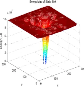
1.1 Energy map of a static sink after first node death . . . 4
2.1 Network lifetime improvement techniques . . . 9
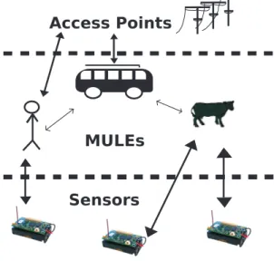
2.2 Mules with three-tier architecture . . . 12
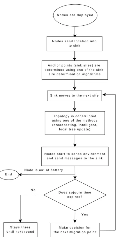
3.1 General scheme . . . 20
3.2 Neighbor based determined sink sites with dominating set heuristic 25 3.3 Coordinate based determined sink sites using squares . . . 27
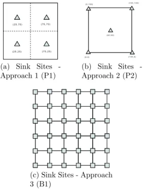
4.1 Different sink site selection approaches. . . 38
4.2 Sink site determination approaches: network lifetime comparison. 39 4.3 Sink site determination approaches: data latency comparison. . . 40
4.4 Network lifetime for different energy levels. (SSD = DSH and tx = 30m). . . 41
4.5 Network lifetime for larger energy levels. (SSD = DSH and tx = 30m). . . 42
4.6 Network lifetime without any movement constraint (SSD = DSH and tx = 35m). . . 43
4.7 Data latency values for varying number of nodes (area side = 300m
and tx = 35m). . . 44
4.8 Energy map of VMM approach after first node death . . . 45
4.9 Energy map of MM approach after first node death . . . 45
4.10 Energy map of RM approach after first node death . . . 46
4.11 Energy map of StS approach after first node death . . . 46
4.12 Network lifetime with varying dmax values (SSD = DSH and tx = 35m). . . 47
4.13 Network lifetime for 400 nodes (SSD = DSH and tx = 30m). . . . 48
4.14 Network lifetime for different topology construction mechanisms (area side = 100m and tx = 15m). . . 50
4.15 Average hop count values for different topology construction mech-anisms (area side = 100m and tx = 15m). . . 50
4.16 Network lifetime for different topology construction mechanisms (area side = 300m and number of nodes = 500). . . 51
4.17 Network lifetime performance of entire scheme (area side = 300m and tx = 30m). . . 52
4.18 Participating Node Percentage in Topology Construction with Lo-cal Tree Update Mechanism . . . 53
4.19 Average Hop Count to Sink Values for Different Topology Update Mechanisms . . . 53
List of Tables
2.1 General comparison between controlled and uncontrolled mobility. 14
3.1 Network lifetime elongation elements proposed in the thesis . . . . 22 3.2 Neighborhood relationships of a sample toy network . . . 24
Introduction
The emergence of tiny sensor nodes as a consequence of the advances in micro-electro-mechanical systems has introduced the wireless sensor networks. Sensor networks consist of hundreds, even thousands of sensor nodes which are deployed to an area of interest and construct a multi-hop network topology in order to achieve a goal. A sensor network has typically two different kinds of nodes: sink and sensor nodes. A sensor node is a low cost, low power device that is responsible from sensing and communicating. Sink node (base station)1
is the node where data are collected and interpreted. Generally, in the literature, it is assumed that sink node has sufficient amount of energy which cannot be depleted during the network operation.
Each sensor node has mainly three basic units in order to achieve its task: sensing, processing, and communication [1]. A node can use different kind of sensors in its sensing unit for interacting with the medium and gathering data related to assigned task. After sensing, a node can process the data (applying various functions like max, min, average) using its processing unit and transmit the data to its parent. It can also receive and relay its children’s packets destined to the sink node. Base station receives and processes all of these packets, and an application that can run on the computer should interact with it and enable the
1Sink
and base station are used interchangeably throughout the thesis
CHAPTER 1. INTRODUCTION 2
end user to display and query the current and past information about the area of interest.
There are various types of sensor network applications. [1] categorizes these applications and gives typical examples for each category. Here we briefly sum-marize these applications.
• Military Applications: The rapid deployment, self-organization and fault tolerance characteristics of sensor networks make them appropriate for mil-itary purposes. Monitoring friendly forces, battlefield surveillance, recon-naissance of opposing forces, targeting, and nuclear and chemical attack detection are examples of military applications. They can be used in hos-tile environments where it is too dangerous for humans to operate.
• Environmental Applications: The most widely used sensor network applica-tion is environmental monitoring. Various types of sensors enable the nodes to sense the environment and perform given tasks continuously. This kind of application includes forest fire and flood detection, habitat monitoring, tracking the movement of targeted animals.
• Health Applications: Some of the health applications for sensor networks are integrated patient monitoring; diagnostics; drug administration in hos-pitals; monitoring the movements and internal processes of small animals; telemonitoring of human physiological data (heart rate, blood pressure de-tection, so on); and tracking and monitoring doctors and patients inside a hospital.
• Home Applications: Sensor nodes can be used for home automation to provide smart home environment in which all the appliances can interact with each other and be controlled remotely outside the home.
• Commercial Applications: This type includes managing and controlling in-ventory, detecting and tracking vehicles, and factory process control and automation.
Wireless sensor networks have special characteristics that differentiate them from ad hoc networks [1, 36]. The number of sensor nodes deployed to the area of interest is much higher (even order of thousands or more in some cases) than that of ad hoc networks. The data communication is generally many to one (each data packet is destined to sink in order to be processed and interpreted) whereas in ad-hoc networks each node can communicate to one another (point-to-point). Deployed sensor nodes can be inaccessible due to harsh environmental conditions in some of the applications of WSN, like forrest fire detection, and battlefield surveillance. In this case, cost of replacing the battery of a sensor node can be more expensive than deploying a new sensor node to the area. The other important difference is the limited computational and memory characteristics of sensor nodes. This property restricts the programmers that design algorithms for sensor networks in order not to exceed the limits of node memory and processing capabilities (a typical Mica2 mote [13] has 128 KB programming memory).
Beside all of these differences, the most important characteristics of WSNs is limited energy resources of sensor nodes. A typical sensor node has generally irre-placeable limited capacity battery attached to the programming interface board. Consuming less amount of energy is the most critical criterion when designing any sensor network related protocol. Since the energy is the most precious re-source, and in most of the applications, replacing the batteries are very hard or impractical, utilizing each node’s and total energy of the network becomes much more important for a given task.
Several schemes are proposed in the literature in order to minimize the total energy consumption in the network for improving the network lifetime: power adjusting when transmitting messages [9], developing energy efficient MAC or routing protocols [14, 30, 41, 42], minimizing the number of messages traveling in the network (since most of the energy is consumed when transmitting data packets), putting some sensor nodes into sleep mode and using only a necessary set of them for sensing and communication [50].
Making the sink mobile appears as another approach for improving the net-work lifetime for WSNs. In a WSN, each sensor node not only transmits its own
CHAPTER 1. INTRODUCTION 4
packet to sink, but also relays the packets of its children, when data aggrega-tion2 3
is not used. Since most of the time a tree topology is constructed from up to bottom (from base station to leaf nodes), all packets of the network are delivered to the sink node via its first hop neighbors. As it can be seen from Fig. 1.1, snapshot of the energy map in the network after first node died, this situation causes these nodes to deplete their energy faster than the other nodes in the network. So, the main motivation behind the sink mobility is to change these nodes periodically (in each round) in order to delegate sink’s neighbor role among the sensor nodes in a fairly manner for balancing the remaining energy level of the nodes and finally improving the network lifetime. A node that was sink’s neighbor in the previous round should have smaller packet load in the next round so that on the average all nodes have nearly equal packet load (so equal remaining energy levels) at an arbitrary time.
Figure 1.1: Energy map of a static sink after first node death
A sink mobility scheme has to address the issue of when (round duration, sojourn time) and where (migration point, sink site, anchor point) to move the sink node next questions and also it should explain which network parameters should be used in order to regulate this operation.
2
Data Aggregation is the process of expressing data in summary form.
3
Each node processes its child’s packet, applies a function to both of its own packet and that of its child (min, max, avg, etc.) and finally transmits one and only one packet to its parent in this case.
1.1
Motivation
Sink mobility has been drawn the attention of the researchers for a few years. Several papers have been published about different aspects of the topic. In order to solve when and where questions of the mobility scheme, to the best of our knowledge, all of them either uses Linear Programming (LP) or Integer Linear Programming (ILP)/ Mixed Integer Linear Programming (MILP). Although this situation provides optimal solution to the given problem formulation and assump-tions, they also bring scalability problem together. Except [3], none of proposed solutions exceeds a hundred number of nodes (whereas [3] uses at most 600 nodes) in their simulation scenarios, which can be treated ”insufficient” when consider-ing the typical sensor network applications like environmental monitorconsider-ing and battlefield surveillance where hundreds or even thousands of nodes are deployed to the area of interest. When the number of nodes increases, time needed for the solution of formulation (which also equals the time elapsed while sink is decid-ing where to move) increases exponentially. Since sensor nodes cannot transmit or receive any data packet during the decision and movement phase, a huge-size buffer requirement problem arises which also increases delay. Due to limited com-putational and memory characteristics of sensor nodes, scalability problem makes those approaches impractical for the applications that require very large number of nodes.
Because of the buffer and delay problem described above, the sink node should not move to points far away from the location that it currently stays, since moving to a distant location also takes time. However, depending on the application, the area of interest that the nodes are deployed can be very large (order of kilometers). On the other hand, some regions of the area (hill, boggy) should have difficulties that prevent the sink node to move a point which lies on this kind of areas even they are closer to the current staying point. These conditions restrict the points that the sink node can move when it wants. To the best of our knowledge, a dynamic sink site determination algorithm has not been proposed before, in which such network parameters are taken into consideration. In previous works, the area of interest is assumed to have square properties, and the corners and
CHAPTER 1. INTRODUCTION 6
some predefined points in this square are defined off-line as the possible migration points independent from any topological or deployment information. However, as mentioned above, these predefined points should have some restrictions to move (no alternative points are given in those works). We have proposed two different sink site determination algorithms which consider number of nodes and their positions (and some probable special conditions) when deciding possible migration points.
1.2
Contributions
In this thesis, we propose a set of algorithms for different aspects of the sink mo-bility problem in wireless sensor networks. First, we propose two different sink site determination algorithms. To the best of our knowledge, these are the first proposed algorithms in which possible sink sites are not given as the predefined points of the area, instead, they will be determined according to the distribution of nodes in the area and their coordinates or neighborhood information. Sec-ondly, a cost function is introduced and an algorithm is given when the buffer size limitation of sensor nodes prevents the sink to move to any candidate site. Additionally, an energy efficient topology construction algorithm and local tree topology construction algorithms are presented which are important for improv-ing network lifetime. These issues were not addressed all together in most of the previous studies.
1.3
Thesis Structure
In Chapter 2, some preliminary information about wireless sensor network is given. The chapter also gives a brief explanation of the previous related work about different general approaches for improving network lifetime (other than sink movement), mobility schemes in general, and specifically sink mobility issue in wireless sensor networks. Pros and cons of each work has been discussed in
detail. Chapter 3 presents the heuristic algorithms about the sink mobility issues with sink site determination, efficient topology construction and local tree update mechanism. In Chapter 4, details about the simulation environment and param-eters are given and results of the experiments are presented. Finally, Chapter 5 concludes the thesis and gives future research directions.
Chapter 2
Background and Related Work
Sink mobility is one of the approaches, among many others, that have been used for prolonging network lifetime. It has been extensively discussed over the last few years by treating one or more different aspects of the network, such as routing, sink location, sojourn time of the mobile sink, etc. In this chapter, important articles that are closely related to our work in this thesis are discussed. However, it is first preceded by a section that classifies the works related to network lifetime improvement and cites some of the important papers in each group.
2.1
Network Lifetime Improvement Approaches:
A Summary
Since energy is the most precious resource of a sensor network, it should be carefully taken into consideration in any algorithm or approach related to sen-sor network operations. This situation causes researchers to deal with network lifetime improvement in different aspects of networking. Before going into more detail about the works related to our study, it would be better to give a brief sum-marization about the papers that use different mechanisms to improve network lifetime. These works generally lie in physical layer (power control), data link
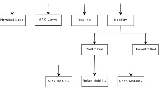
layer (MAC protocols), network layer (routing), or upper layers (data gathering, clustering). Most of the papers deal with one of the aspects that lie only in one layer, whereas some other works [5, 23, 24, 32] use cross-layer design where differ-ent issues related to more than one layer are taken into consideration in order to maximize network lifetime. Fig. 2.1 shows a brief description of network lifetime maximization techniques. N e t w o r k L i f e t i m e I m p r o v e m e n t A p p r o a c h e s P h y s i c a l L a y e r R o u t i n g M o b i l i t y U n c o n t r o l l e d C o n t r o l l e d M A C L a y e r S i n k M o b i l i t y R e l a y M o b i l i t y N o d e M o b i l i t y
Figure 2.1: Network lifetime improvement techniques
Since communication is the main source of energy consumption, efficient power management while transmitting and receiving messages can effectively extend the operational lifetime of the network. Different mechanisms are used in order to achieve this task. [55] combines both routing and power adjustment mechanisms for network lifetime improvement. It basically proposes a routing mechanism in which each node adjusts its transmission power to send packets to its neighbors. [56] tries to evenly distribute the traffic load by dividing the area to ring zones and resets the transmission radius of each node according to which zone it belongs to. [10] emphasizes that sensor nodes are generally densely deployed to the area of interest, and therefore targets are redundantly covered. It adjusts the sensing ranges of sensor nodes and aims to find maximum number of set covers and the ranges of each sensor in this set such that each set covers all the targets.
CHAPTER 2. BACKGROUND AND RELATED WORK 10
Numerous MAC protocols are proposed in the literature that consider the spe-cial characteristics of wireless sensor networks. Almost all of them carefully treat the energy issue in sensor nodes and propose energy-efficient MAC layer proto-cols. These energy efficient protocols directly contribute to the network lifetime, since they avoid redundancy in typical operations of this layer (synchronization, control packet exchange, etc.). [14, 30, 38] are some important and widely used energy-efficient MAC protocols in the literature (more protocols, their pros and cons and comparison table, and causes of energy waste at this layer can be exam-ined in a related survey paper [16]). Unlike the others, [33] proposes an adaptive MAC protocol that guarantees network lifetime for wireless sensor networks. It both guarantees the pre-configured network lifetime and reduces end-to-end la-tency by introducing an adaptive duty cycle depending on ratio of the remaining energy to the initial energy considering the pre-configured network lifetime.
Routing is another area that researchers concentrate in order to improve net-work lifetime. [11] states that energy consumption rate per unit information trans-mission depends on the choice of the next hop if the transtrans-mission power level can be adjusted. It proposes a shortest cost path distributed routing algorithm that uses link costs in which residual energy levels between two nodes are consid-ered. [35] shows that the problem of routing messages in a sensor network in order to maximize network lifetime is NP-hard. They develop an online heuristic to maximize network lifetime which also provides larger network capacity. [51] emphasizes that performance of sensor networks are related to both time (net-work lifetime) and space (net(net-work coverage - source level fairness) domains. The authors develop simple, localized, and a probabilistic protocol which addresses performance issues in both time domain, by exploring multiple paths when send-ing messages for uniform energy consumption, and spatial domain, by reducsend-ing the load over congested nodes.
There are another classes of approaches, other than these three major ones, which are used for improving network lifetime. Topology control [2, 29], data gathering and aggregation [15,25–28,57], clustering [17,21,37], and sleep schedul-ing mechanisms [7,45,54] can be given as examples for these classes. Sink mobility has been emerged as another approach in this domain for the last few years.
2.2
Sink Mobility for Network Lifetime
Im-provement
Although the goal of all the approaches mentioned in the previous section are same, they differ in the way they consider the resulting energy consumption be-havior in the network. [47] categorizes energy consumption strategies while deal-ing with network lifetime. Most strategies aim to minimize average, maximum, or relative energy consumption by using a related technique. Some routing pro-tocols (reducing the transmission cost of a packet via optimal route) and power management techniques (each node adjusts its transmission power while sending a message) minimize the maximum energy consumption, while some energy ef-ficient MAC protocols minimize average energy consumption (all nodes use the same sleep/idle schedules and reduce the average energy consumption). As stated in [47], in most studies neither average nor maximum strategies consider current energy status of a node. That is why, they cannot avoid the nodes whose their batteries are getting exhausted to die. Unlike these approaches, in (controlled) sink mobility, current remaining energy values of sensor nodes are taken into con-sideration, and this helps to extend the lifetime of nodes as much as possible. This brings a serious advantage in the case that network lifetime is defined as the time passed until the first node depletes all its energy, which is commonly used definition in the literature.
Sink mobility can be classified into two categories according to the moving strategy used: uncontrolled (random), and controlled [4, 19].
2.2.1
Uncontrolled Mobility in Wireless Sensor Networks
Uncontrolled mobility is the scheme used when mobility in wireless networks has been introduced to WSN domain [22, 43]. In this type of mobility, a third tier is used in the network (as seen in Fig. 2.2 - redrawn from [22]), in which mobile agents (a.k.a. MULEs - Mobile Ubiquitous LAN Extensions) are deployed between access points (base stations) and sensor nodes in order to collect data
CHAPTER 2. BACKGROUND AND RELATED WORK 12
from sensor nodes when in close range, buffer them and finally transmit them to the sink [43]. It is called as uncontrolled, since movement is random and MULEs (for instance vehicles) move according to their needs and only exchange data if they encounter any node as a result of their movement [22, 43]. The main motivation behind MULEs is to reduce energy cost for data transmission by using single-hop communication (from node to MULE or MULE to sink), instead of the more expensive multihop routing. Since communication cost is the most energy consuming part in network operations, this approach effectively increases network lifetime. However, since the arriving time of any MULE (either to a node or to the sink) is not known a priori, this causes two important problems: large size of buffers that nodes should have, and large data latency. Sensor nodes should have large buffers in order to save all packets generated between two consecutive visits of the MULE. It is also unpredictable when a MULE comes close to the sink node and transmits packets to it. This can cause a huge delay between the time that data is generated and received by the sink. It is obvious that there is a trade-off between latency and energy consumption. If our application is delay tolerant, then uncontrolled sink mobility becomes a good option. Packet loss risk should also be evaluated if nodes do not have large enough buffers that can save all the packets generated between two consecutive visits of a MULE.
MULEs
Sensors Access Points
2.2.2
Controlled Mobility in Wireless Sensor Networks
Contrary to its counterpart, in controlled mobility, movements are done depend-ing on the conditions of the network (like current energy map, node density in the regions, etc.). Currently, there are three main approaches used in controlled mobility [3]. In first and mostly used one, the sink moves among the nodes and collects data without any additional entity (which is also the case in this thesis). In the second approach, mobile relays are used as forwarding agents - like MULEs, but in a controlled manner in this case - for the communication between sensor nodes and the base station [46, 48]. In the third approach, sensor nodes them-selves are mobile [49,52]. Generally, sink node or relay nodes are assumed to have more powerful energy resources such that their energies are not being depleted during the network lifetime. Therefore it is expected that mobility of these types of nodes does not adversely affect the network lifetime. However, for sensor nodes this is not the case. As it was mentioned before, sensor nodes have very limited energy batteries, which cannot be wasted for mobility, topology reconstruction, etc. unless it is certainly necessary. That is why, the first two approaches appear to be the more promising for energy efficiency and longer network lifetime [3].
Controlled and uncontrolled mobility in WSN domain is compared against each other using some performance measures in [4]. As discussed above, uncon-trolled mobility has higher data latency but lower energy consumption than that of controlled one. When network traffic is low, deployment area is small, buffer size is large enough and MULE speed is quite fast, there is no packet loss in both approaches. However, as the deployment area grows and/or MULE becomes slower (inter-arrival time at the same cell increases), overflows occur in sensor node’s buffers and packet delivery ratio decreases as a result. Moreover, since movements are done in random manner in uncontrolled mobility, computational cost is lower than that of controlled one. As a result, both mobility schemes have pros and cons. Basic comparison is summarized in Table 2.1 from [4]. Choosing the appropriate scheme completely depends on the application that we have. If we can tolerate data latency and some possible packet losses and/or we have rel-atively small deployment area and MULEs travel faster in that area, than it will
CHAPTER 2. BACKGROUND AND RELATED WORK 14
be important to use data MULEs for communication in order to effectively reduce the energy consumption. However, if we have a critical application (which is the case in our work) that is intolerant to any latency or packet loss, like earthquakes, fire detection, or battlefield surveillance, then controlled mobility (via either re-lays or sink) become crucial. In this thesis, we focus on controlled mobility , and we propose algorithms for controlled sink mobility case, mobile relays are out of the scope of this work.
Controlled Uncontrolled Data latency Low High Energy Consumption Medium Low Computational Needs Medium Low
Table 2.1: General comparison between controlled and uncontrolled mobility.
2.2.3
Controlled Sink Mobility
In this work we focus on the case where sensor nodes are stationary and there is not any additional tier, instead just the sink is mobile and moves among different migration points. However, movement of the sink depends on different parameters of the network (hence it is controlled). There are different works done in this track that deal with issues regarding sink mobility.
[18] examines sink mobility problem with multiple base stations (unlike our case, where we have one mobile sink). The main motivation behind this choice is to have more options for routing and reducing and retaining the hop count (so energy consumption). It presented two different integer linear programming (ILP) formulations, which have objective function either to minimize the maxi-mum energy spent by a sensor node (BSLmm) or to minimize the total energy
consumption (BSLme) in a round subject to some constraints, for relocation of
the multiple mobile sinks (maximum 3) in each round (equal period of time, T timeframes) to prolong the lifetime of the sensor network. The paper evaluates the performance of the static and mobile approaches with 3 mobile base stations.
Since lifetime is defined as time until first node dies, (BSLmm) outperforms other
four schemes. They also examine the impact of the number of available base stations over the network life time and see that increasing the number of base stations beyond a certain threshold value does not improve the network lifetime (since at that time there are sufficient number of base stations in the network such that each sensor node can transmit messages via single hop communication). Mobility and routing are considered together in [31]. It is assumed that sensors are densely deployed (as a Poisson process with density ρ) within a circle. They define the network lifetime as the time span until the first loss of coverage. The authors prove that, the center of the circle is the optimum location for the sink in terms of energy efficient data collection and mobility helps to balance the load and prolong the network lifetime. They define the problem with a linear programming formulation (minimizing the load on each sensor node N), and solve it first finding the optimum mobility strategy by fixing the routing strategy as shortest path routing, then use the output strategy in order to find the final routing strategy with better performance than shortest path one. After the claims and proofs which limit the mobility trajectories, finally it is proved that optimum mobility strategy is the trajectory around the periphery of the network. The authors find a ’better’ routing strategy by concentrating on an inner circle in the network area and develop a heuristic using this structure. Simulations are done in order to see how results from the analytical analysis overlap with those coming from the simulation. Since there is not any result related to a comparison with any other mobility approach (like random), we cannot make comment about the performance of the proposed scheme. The main drawback of the work is the assumption that network region is circular. There is not any discussion that explains how the solution is transferred to another region types in the paper.
One of the works closer to our work is presented in [34]. In this paper, N sensor nodes and a sink node s are randomly deployed to an area of interest. There is a constant information generation rate at every sensor node and a set of locations where the base station can move and stay. The authors present two complementary algorithms for solving the sink mobility and routing problem to-gether. One is the scheduling algorithm that determines the duration for each
CHAPTER 2. BACKGROUND AND RELATED WORK 16
candidate sink site that the base station can stay, and the other is the routing algorithm in order to find the energy-efficient paths for each packet from a sensor node to the sink. Linear Programming (LP) formulation is given which maxi-mizes network lifetime, the sum of sink sojourn times at all possible locations, subject to some constraints and compare mobile and static sink approaches with different routing schemes. In simulations, there are two scenarios including just four (centers of four sub-squares) and five different (corners and center) sink sites, respectively. Experiments are done and compared via adding the routing parame-ter which prevents us to observe the performance of the proposed mobility model in the paper.
One of the more recent and detailed work about controlled sink mobility is presented in [3]. They present a centralized Mixed Integer Linear Programming (MILP) model that determines sojourn times and order of the visits to sink sites. Moreover, one of the first fully distributed and localized heuristic called Greedy Maximum Residual Energy (GMRE) is developed as a solution of the same problem. Network model is quite similar to the one given in [34]. Unlike that model, deployment area is divided into grids and the corners of these grids are determined as sink sites. They introduce two different parameters in order to make the model more realistic. The dM AX parameter represents an upper
bound for the distance between the current and next site that sink can travel. This parameter bounds the time of the sink movement and enables the sensor nodes to save the packets in buffer without any loss. MILP formulation aims to maximize total sojourn time, as in [34], subject to some constraints. They evaluate the performance of MILP, GMRE, Random Movement (RM), and Static Sink approaches. MILP and GMRE gives better results than the others. MILP performs better than GMRE between 30% to %50 (for increasing tmin values).
Previous works that use (Mixed) Integer Linear Programming force the au-thors to limit the number of sink sites and number of nodes in their simula-tions. [18] uses maximum 30, while [34] uses 100 nodes in their simulasimula-tions. Since Integer Programming/Mixed Integer Programming is NP complete [53], increas-ing number of nodes will cause very long delays durincreas-ing the sink decision process. However, it is more likely to deploy order of ten-thousand nodes to a terrain in
a classical WSN application (especially when the cost of a sensor node becomes cheaper), and it is unrealistic to neither expect each sensor node has infinite or very large buffer capacity (since they have limited resources) that will not waste the packets during migration decision process, nor tolerate such a large delay for most of the typical WSN applications. Heuristic algorithms can be more ad-vantageous and effective in this case than the optimal solution with less realistic assumptions, especially for very large number of nodes.
In this chapter, network lifetime improvement approaches are summarized using the networking layers perspective: physical, datal link (MAC), network, and upper layers. Important works in each group are explained briefly. Sink mobility is one of the approaches that lie in application layer. Uncontrolled and controlled mobility is discussed in detail. Since our work is in sink mobility part, related work in this area is given. The drawbacks of these works, which are the reasons behind the motivation of this thesis, are also discussed.
Chapter 3
Our Solution
Our goal with this thesis is to propose a set of algorithms for different aspects of the sink mobility problem in wireless sensor networks in order to improve network lifetime. Briefly, in this chapter, first our general algorithm and its steps are presented preceded by the network model and the problem definition. After that each sub-algorithm will be given in detail.
3.1
System Model and Problem Definition
We consider a wireless sensor network that has N static sensor nodes and a mobile base station. Sensor nodes are deployed to the region of interest in a random manner. After the mobile sink moves to its initial location, it broadcasts messages in order to construct a routing topology, from up to bottom. Each node, that receives the message, which means each node in the transmission range of the sender, re-broadcasts the message, putting its ID as ’parent ID’ to the related part of the packet. Each node that receives the broadcast packet saves the parent ID. After the topology construction, nodes start to sense the environment. There is a constant packet generation rate Qi for each sensor node i ∈ N. There is no
data aggregation in the network; that is each parent relays its children’s packets to the sink. Base station knows the exact location of the sensor nodes using an
available technology like GPS or GPS-less [6,39,40] localization algorithms. Each packet will be received by the sink which implies there is no packet loss in the network (perfect MAC layer). Each sensor node has enough buffer size in order to avoid loosing packets during the traveling time of the sink from the current site to the next one (or this time is negligible). In this work, we define the network lifetime as the period of time until the first node dies, which is commonly used in the literature.
We present different heuristic based algorithms in order to bring a new ap-proach to the sink mobility issue using the answers of three questions:
-When the sink decides to move to another site? -Where the sink will go to as new site?
-How the sink decides to move or stay (obtaining the parameters)?
To decide when to move, generally, we use remaining energy level changes in the neighbors of the sink.
In typical sensor network applications (like forest fire detection), hundreds or even thousands of sensor nodes can be deployed to the region of interest. This area can be very large such that it should be very difficult to consider each node point in the area as a candidate sink site (point within the deployment area the sink can visit), since this will dramatically increase the time to decide whether to stay at the current point or move to another point in the area (and where to move if it does not stay). However, the decision process should be completed as quickly as possible. This requires determining a set of S = 1, . . . , q sink sites after the deployment, and consider only those points when deciding to change position in the area.
The main motivation behind the sink site determination algorithms is to de-crease the candidate migration points in the deployment area the base station
CHAPTER 3. OUR SOLUTION 20 N o d e s a r e d e p l o y e d N o d e s s e n d l o c a t i o n i n f o t o s i n k A n c h o r p o i n t s ( s i n k s i t e s ) a r e d e t e r m i n e d u s i n g o n e o f t h e s i n k s i t e d e t e r m i n a t i o n a l g o r i t h m s S i n k m o v e s t o t h e n e x t s i t e D o e s s o j o u r n t i m e e x p i r e s ? N o S t a y s t h e r e u n t i l n e x t r o u n d Y e s M a k e d e c i s i o n f o r t h e n e x t m i g r a t i o n p o i n t T o p o l o g y i s c o n s t r u c t e d u s i n g o n e o f t h e m e t h o d s ( b r o a d c a s t i n g , i n t e l l i g e n t , l o c a l t r e e u p d a t e ) N o d e s s t a r t t o s e n s e e n v i r o n m e n t a n d s e n d m e s s a g e s t o t h e s i n k E n d N o d e i s o u t o f b a t t e r y
can visit in order to minimize the decision time, in other words reduce the com-putational cost, when deciding the next sink site after the sojourn time1
expires. In some scenarios, sensor nodes are deployed to an area where some points can be inaccessible or very difficult to access. This implies that sink can not visit any point in the deployment area due to some harsh environmental conditions. These reasons force us to choose sink sites before network starts operating.
In the literature, as in [3, 34], the deployment area is divided into grids (like 4x4 or 8x8) and sink sites are determined as the corners of those grids without any computation. However, it would be better to determine those sites with more intelligent algorithms using the current deployment or neighborhood information. In a network without data aggregation, nodes within the transmission range of the sink are going to relay the packets of all the nodes that are under the lower levels of the logical tree topology. This causes those nodes to deplete their energy faster than the other nodes. That is why the most important thing to consider is to group (cluster) those nodes and choose a point in such a group when determining the sink sites. By this method, we should balance the energy consumption of this first order nodes and prolong the network lifetime.
3.2
General Scheme
This thesis gives a set of algorithms for sink mobility and some related problems, as itemized in Table 3.1, in order to improve network lifetime. The big picture of the network operations are given in Fig. 3.1. First solution is about sink mobility which consists of both sink site determination and movement criterion. We present two different sink site determination algorithms. Each algorithm uses different mechanisms in order to choose sink sites. After that, both algorithms use the max-min based (maximum of the minimums) approach or its modified version (visit added) for moving from one point to another. Another solution we propose is a tree topology construction algorithm which aims to fairly distribute
1
CHAPTER 3. OUR SOLUTION 22
the packet load among the nodes by considering the remaining energy informa-tion. Finally, our local tree topology update algorithm tries to prevent redundant message exchanges inside the network when topology is being reconstructed at each movement of the sink.
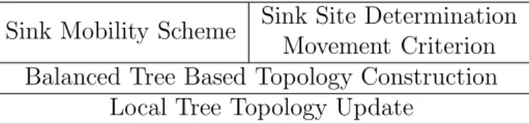
Sink Mobility Scheme Sink Site Determination Movement Criterion Balanced Tree Based Topology Construction
Local Tree Topology Update
Table 3.1: Network lifetime elongation elements proposed in the thesis
3.3
Sink Mobility Scheme
Sink mobility scheme has two major steps: finding candidate migration points (sink sites), moving through these migration points. For the first step, two differ-ent sink site determination algorithms are presdiffer-ented which are based on locations (coordinates) of the nodes on the deployment area, and on neighborhood relation-ships, respectively, in the following two sections. After that, how (using which parameters and how to obtain them) and when to migrate to those points are discussed. Finally, a cost function is introduced in order to examine the problem of how to choose a new migration point from a set of points when the nodes have limited buffer capacity.
3.3.1
Sink Site Determination
After hundreds of nodes are deployed to an area of interest, there is infinite num-ber of points in the area that sink can move. The numnum-ber of possible points will be in the order of hundreds, even we limit the points to the coordinates of the sensor nodes. Large amount of candidate points causes too much compu-tational cost while deciding where to move at the end of each round. If sensor
nodes do not have an infinite buffer (or sufficiently large one that can store all generated traffic during decision process), and if decision takes too long, loosing data packets becomes inevitable. There can be lots of applications which cannot tolerate such a case. Also, because of some typical sensor network applications (like environmental monitoring), nodes can be deployed to areas that can have harsh conditions (like boggy, hilly) into which the sink node cannot move. All these cases require to select some set of points (i.e. sites, anchor points, candidate migration points) that the sink node can potentially migrate before the network starts to transport data.
To the best of our knowledge, there is not any study about sink mobility that includes a dynamic sink selection process. All of them are off-line and does not include any detail about the deployment of sensor nodes or other physical conditions. Most of them just use corner points of the square or grids in the area [3, 34]. Unlike other works, by these two algorithms, we try to give different sink site selection mechanisms which treat the network conditions as well.
3.3.2
Neighborhood Based Sink Site Determination
Algo-rithm
Sometimes, it can be difficult to know the exact boundaries of the deployment area and the coordinates of each sensor node in the region. In this case, the neighborhood information of the nodes can be used for determining candidate sink positions. Since every node receive/hear messages during network operation, or can exchange neighborhood information using control packets, each node can know its neighbors independent of their coordinate information.
Since the main motivation of sink mobility is to evenly distribute the heavy load of the base station’s neighbors, we want to group those nodes via an algo-rithm in order to be chosen as sink’s neighbors. The neighborhood relationships are used for solving this problem. If we are given n nodes and neighborhood re-lationship information, then our aim is to choose q nodes from the list such that,
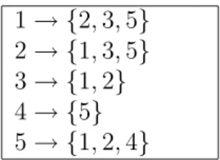
CHAPTER 3. OUR SOLUTION 24 1 → {2, 3, 5} 2 → {1, 3, 5} 3 → {1, 2} 4 → {5} 5 → {1, 2, 4}
Table 3.2: Neighborhood relationships of a sample toy network
union of the neighbors of these nodes cover all the nodes in the area. This pro-cess is quite similar to finding a dominating set for a graph G = (V, E), which is defined as every vertex not in dominating set D is adjacent to at least one vertex in D [8]. Dominating set problem is a special instance of set covering problem, and it is NP-complete [44]. 2
A sample neighborhood relationship of a five node network is given in Table 3.2. Each node’s neighbors are given in curly brackets. We can see {1, 2, 3, 4, 5} as universal set and their neighborhood information as subsets of this set. If nodes 1 and 5 are chosen then, all of the nodes will be covered with repetitions (for 1 and 2)
We present a greedy heuristic algorithm for dealing with dominating set prob-lem. In the beginning, after determining the neighborhood information of each node (either by computing at the sink using coordinates or collecting neighbor information from the nodes to the base station), the sink node sorts the nodes in descending order with respect to their number of neighbors. Then the heuristic algorithm takes the coordinate of the node (a contributed node) with the most number of neighbors in the beginning and put those neighbors to the current neighbor list. After this step, the Algorithm 1, keeps the list of covered and un-covered nodes at each step. After first contributed node is chosen (the node with the most number of neighbors), its neighbors are saved in coveredNodes list. The uncoveredNodes list is simply calculated via taking set difference of universal set (all nodes) and coveredNode list. After initialization of those lists, node that has
2
The decision version of set covering is NP complete, and the optimization version of set cover is NP hard since it generalizes the NP-complete vertex-cover problem [12].
the maximum number of common elements with uncoveredNodes is chosen as the next contributed node. Then its neighbors are added to coveredNodes list and uncoveredNodes list is updated. This iteration continues until uncoveredNodes list becomes empty (coveredNodes equal to universal list). Figure 3.2 shows the possible sink sites (stars) as the output of the algorithm. If we look at the com-plexity analysis of the algorithm, while loop will iterate n − 1 times (where n is the number of nodes) if each node has at least one common element, and inner loop also iterates n times, therefore the complexity is O(n2
) in the worst case.
0 50 100 150 200 250 300 0 50 100 150 200 250 300
Figure 3.2: Neighbor based determined sink sites with dominating set heuristic
3.3.3
Coordinate Based Sink Site Determination
Algo-rithm
In the literature, it is generally assumed that base station knows the exact location of sensor nodes using either GPS modules located on the sensor nodes or GPS-less localization algorithms. With that information it would become possible to group those nodes using their coordinate values on the sink side.
CHAPTER 3. OUR SOLUTION 26
Algorithm 1: Neighborhood based sink site determination algorithm -dominating set heuristic(neighborhoodRelationships)
foreach node i in area do
neighbors[i] = nodes in the transmission range of node i; neighborSize[i] = size(neighbors[i]);
end
sortedIndices ← sort(neighborSize, ‘descendingOrder′);
ind = 1;
contributedNode(ind) = sortedIndices(1);
coveredNodes = contributedNode(ind).neighbors; uncoveredNodes = universalSet − coveredNodes; currentNeighborsList = neighbors(sortedIndices(1)); ind = ind + 1;
while uncoveredNodes = φ do
foreach node i in sortedIndices do
commonElements(i) = size(intersect(neighbors(sortedIndices(i)), uncoveredNodes));
end
indx = index of max(commonElements); contributedNode(ind) = sortedIndices(indx); ind = ind + 1;
coveredNodes = coveredNodes + contributedNode(ind).neighbors; uncoveredNodes = universalSet − coveredNodes;
end
foreach node i in contributedNode do
candidateMigrationP oints(i) = coordinate(contributedNode(i)); end
In the coordinate based sink site determination algorithm, we divide the de-ployment area into squares such that each one’s length is equal to the transmission range. That enables us to group (cluster) the nodes that can be the sink’s neigh-bors in any round and compare their energy levels and decide which subarea to move in the next round. The number of areas is dynamically changing according to the transmission range values.
.
.
.
.
.
.
.
.
.
.
.
.
.
.
.
.
.
.
.
.
.
.
t x*
*
*
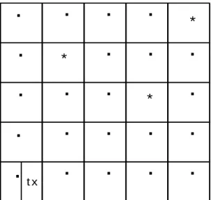
Figure 3.3: Coordinate based determined sink sites using squares
As it can be seen in Fig. 3.3, the distance between any two neighbor sink sites is R, where R is the maximum transmission range. Each sink site is ideally placed at the center of the allocated area. The detailed algorithm is given in Algorithm 2. After determining the centers of each sub square, sparse areas are eliminated if their density is below the threshold, where threshold is determined by dividing the number of nodes to the number of sub squares.
Since each node’s coordinate is known by sink node, the area is not needed to be regularly allocated to the squares in order to use this algorithm. The sink node can choose the node that has minimum (x,y) pair and assumes that it located on the left lower corner of the imaginary sub square. Then it chooses the center of this sub square as candidate migration point, and continues this operation, until all the nodes in the area are covered. Since the algorithm iterates two times over the number of sub squares, its complexity is O(s), where s is the number of sub
CHAPTER 3. OUR SOLUTION 28
squares and is calculated as (edgeLengthOf Square/transmissionRange)2
. A dynamic sink site selection algorithm (either neighborhood or coordinate based) provides us to eliminate the areas that are on inaccessible terrains which prevents sink to move and stay at that point. For instance, in Fig. 3.3, the ones with * are inaccessible areas that have hard physical conditions (boggy area, hills, so on) are eliminated before network operation starts. We also eliminate the parts (in coordinate based part, either square or circle) that do not have any node in the sub area during the algorithm.
Algorithm 2: Coordinate based sink site determination algorithm (nodeCoordinates, txRange)
numberOf Subsquares ←
square(edgeLengthOf Square/transmissionRange); ind = 1;
foreach i ≤ numberOf Subsquares do precmp(i, :) = [xcenterycenter]
end ind = 1;
foreach i ∈ precmp do
if precmp(i, :) is accessible and density ≥ threshold then candidateMigrationP oints(ind, :) = precmp(i, :); ind = ind + 1;
end end
return (candidateMigrationP oints);
3.3.4
Sojourn Time and Movement Criterion
After candidate sink sites are determined, the sink node moves to the densest point of the area (first migration point) and the routing topology (i.e. tree) is constructed (either via broadcasting, or some intelligent topology construction mechanism). Sink gets the remaining energy values from its neighbors in order to learn the minimum energy level in the one-hop neighbors before packets start arriving. Since energy levels are piggybacked in each packet, sink can have the chance of comparing the current minimum energy value and the starting one. If
the difference between them is one or more levels, then the sink starts the decision process to determine the location to move for the next round. The number of energy levels (L) determine the sojourn time of the sink for that location, which is the time until any node spends 1
L of its energy. Too many levels means shorter
sojourn times. For example, if we have small number of energy levels, like 4, then 25% of the node’s energy must be depleted in order to trigger another migration process. Some applications should require a minimum sojourn time on a site in order to ensure data quality. For these cases, we introduce the value tmin, which
is defined as the minimum time that a sink should stay on the current site. Such a dynamic approach is more advantageous than a static approach where fixed number of rounds are used. For instance, sink can immediately move to another site if a sink neighbor has tremendous packet load and dramatically looses its energy, however fixed round approach will wait there until the number of rounds are completed and possibly causes the node to die.
If sojourn time expires (either exceeds tmin or a change in energy level
oc-curs), the sink examines the minimum remaining energy value in each candidate migration point, which means the minimum energy value among the nodes’ en-ergy values that fall into the circles or the squares, using the information in the last received packets. Then it moves to the point where the minimum remaining energy level is maximum among the sites that have not been visited yet (max-min approach). When we say ’have not been visited ’, we mean a site cannot be visited until sink has moved to all of the candidate migration points once. After all visits are done, then the visited flag will be set to zero for all of the sink sites and they all become available to visit again. The motivation behind this approach is this: if we just use max-min approach then we may stuck to a single local maximum and cannot focus more into a general picture. In other words, when we are only interested in energy dimension of the problem, then we can ping pong among a few sink sites and have similar packet load patterns (if a deterministic topology construction algorithm is used like in the next section). However, if we visit different sites, then we can achieve more uniform packet load distribution. Therefore this visit added max-min approach, which is summarized in Algorithm 3, corresponds to visiting possible sink sites with an order in which the node with
CHAPTER 3. OUR SOLUTION 30
maximum of the minimum energy values in the sites takes precedence. Since the algorithm iterates over the number of migration points (m), and calculates minimum energy among the nodes on each site, its complexity is O(m · n) (where n is the number of nodes) in the worst case.
Algorithm 3: Migration criterion - visit added max-min approach notV isitedList = migrationP oints;
start with migrationP oints[0];
notV isitedList = notV isitedList − 0; while first nodes depletes its energy do
update EnergyList after transmissions;
if energyLevelChange of any node j >= 1 then foreach point i in notV isitedList do
neighbors[i] = nodes in transmission range of migrationP oints[i];
foreach node k in neighbors[i] do energyList(k) = energy of node k end
end
minimumEnergyNode = index of min(energyList)
minimumEnergyList[i] = minimumEnergyNode newIndex = index of max(minimumEnergyList);
nextSite = notV isitedList[newIndex]
notV isitedList = notV isitedList − newIndex; if notV isitedList == φ then
notV isitedList = migrationP oints; end
migrate to nextSite; end
end
3.3.5
Introducing Cost Function
Some applications can require high number of sensor nodes that are deployed to an area that can be order of tens of kilometers square. In that case, movement time of the sink from one point to another should increase dramatically. This situ-ation directly affects other nodes since they continue sensing the environment and generating packets. Because of not using data aggregation, high data generation
rate (like a packet for each second) causes each node to buffer many packets until the sink node reaches the new site for the next round. In previous sections, it is assumed that nodes have unlimited buffer capacity and do not loose packets, and therefore the sink node can move to any migration point in the area. However, in real scenarios, this is not the case. Sensor nodes have limited buffer capacity and after a while they start loosing packets when new packets enter to the queue. For some critical applications, including battlefield surveillance, earthquake and fire detections, it is generally undesirable to loose any single packet. This forces us to define a cost function. For instance, assume that the sink node is on a vehicle which has a speed of 1 m/s. Each sensor node has buffer capacity of, say 50 packets, and packet generation rate Qi is 1 packet per second. In this case,
if we ignore the topology reconstruction time, this means that the sink node can move to a point that is at most 50 meters (called dmax) away from its current
position without loosing any packet. For such cases, we propose to consider only the set of nodes inside a circle of dmax radius as candidate migration points, and
try to move to one of them which is the most energy efficient. This approach is summarized in Algorithm 4. In the worst case scenario, its complexity is O(m · n) where m is the number of migration points and n is the number of nodes.
Algorithm 4: Centralized migration algorithm with cost function foreach point i in migrationP oints do
neighbors[i] = nodes in transmission range of migrationP oints[i]; foreach node k in neighbors[i] do
energyList(k) = energy of node k end
minList[i] = index of min(energyList); end
maxIndex = index of max(minList) ; newSite = migrationP oints(maxIndex); migrate to newSite
CHAPTER 3. OUR SOLUTION 32
3.4
Load Balanced Topology Construction
Al-gorithm
Usually tree-based routing topology is constructed using a broadcast mechanism as follows: after the mobile sink moves to its initial location, it broadcasts mes-sages in order to construct the topology from up to bottom. Each node that receives the message, which means the node is in the transmission range of the sender, re-broadcasts the message after putting its ID as ’parent ID’ to a field of the packet. Each node that receives the broad-cast packet saves the parent ID.
In the approach above, current energy levels of the nodes are not taken into consideration. Proposing an intelligent algorithm, which considers the current energy level and packet load of the nodes should yield a better network lifetime. Algorithm 5 gives a balanced tree based topology construction mechanism. Sink’s neighbors are in the first level in the logical tree, neighbors of its neighbors are in the second level, and so on. For each node in level l, if a neighbor node is in the logical level l − 1, it becomes a candidate parent and its ID is put into the parent list. After calculating these values, the algorithm is started to run in the last logical level of the tree, namely leaves. Nodes in the last level of the tree are sorted according to the number of candidate parents in ascending order. The main motivation behind sorting the nodes is to give priority to the nodes with less number of options. By this way, when we come to nodes with more options, nodes have updated packet loads, that’s why a better decision can be made among many options. If a node has only one parent in its list, then this node is assigned as the parent node and its packet load is also incremented by the packet load of the child. If a node has more than one candidate parent, the ratio of energylevel/packetLoad2
is calculated for each candidate. The candidate with maximum ratio value is assigned as the current node. Since the algorithm is run from bottom to up, the packet load of the most critical nodes (i.e. sink neighbors) can be determined using the full information of the nodes below.
The algorithm consists of two main for loops. The first loop’s complexity is O(n). The second loop iterates for each candidate parent of each node in
each level in the tree. The outer two loops iterate over the all nodes in the area (iteration is over the nodes level by level). In the worst case, a node can access to all nodes in one hop, therefore its number of neighbors can be equal to n − 1. In this case, we have two loops which iterate for n and n − 1 nodes, respectively, which yields O(n2
) complexity.
Algorithm 5: Load balanced topology construction algorithm sink initiates broadcast;
foreach node i in area do
logicalLevel[i] = hop distance to sink node ;
parentList[i] = nodes which packets reach from upper level; end
for level = bottom to first do
sortedNodeInCurrentLevel = sort(size(ParentList), ’ascendingOrder’); foreach node i in sortedNodeInCurrentLevel do
if size(parentList[i]) == 1 then
nodes[i].parentId = parentList(1, 1); end
else
foreach node j in parentList do
ratio(j) = energylevel(j)/currentP acketLoad2
end
maxRatioIndex = index of max(ratio)
nodes[i].parentId = parentList(maxRatioIndex); end
update packetLoad for the parent end
end
3.5
Local Tree Topology Reconstruction
One of the disadvantages in sink mobility scheme is to re-construct the topol-ogy for each movement of the sink. This will increase the number of con-trol/management packets in the system, which also implies higher overhead. Since each node transmits (broadcasts) and receives a packet during the topol-ogy re-construction process, for short period of sojourn times the number of sink
CHAPTER 3. OUR SOLUTION 34
movements will be increased and energy of each node will be wasted for con-trol packets. For higher number of nodes, this process will be annoying and will take more time and will prevent the sensor nodes from transmitting data packets (instead store them in the buffer) until the topology is fully constructed. This can be a problem for some applications, such as earthquake and fire detection, which do not tolerate delay in transmission of packets. Therefore, for both en-ergy and application specific purposes, local tree topology re-construction can be a necessity in some cases as part of a sink mobility scheme in order to improve network lifetime and decrease data latency. Details of such an algorithm is given in Algorithm 6. When a node receives a packet from sink, it always rebroadcasts the packet, even it was one of the sink’s neighbors in previous round. For others that receive packet from non-sink nodes (i.e. ordinary nodes), it checks whether the sender was its parent in the previous round or not. If it was, then it stops to rebroadcasting packet to the network, otherwise rebroadcasting continues. Since the algorithm iterates over the number of nodes in the area, its complexity is O(n).
Algorithm 6: Local tree re-construction algorithm sink initiates broadcast;
foreach node i in area do
if packet received from sink then re-broadcast the packet with id i end
else
if packet received from parent in the previous round then stop broadcasting
end else
re-broadcast the packet with id i end
end end
The main disadvantage of a local update algorithm is having longer paths than its fully reconstructed counterpart. This can increase the energy needed for a packet while reaching to the sink (number of transmissions should increase). However, for highly mobile environments (sink’s sojourn time is very short or it is
continuously moving), local update mechanism become more advantageous, since topology construction cost increases for full update one.
In this chapter, we define the problem of sink mobility and give the general solution scheme that is used in the thesis. Two different sink site determination algorithms are given for each of the cases that either the sink node does not know the exact coordinates of the nodes (neighborhood based) or it can calculate these coordinate values either with a GPS module or a localization algorithm (coordinate based). After the selection of candidate sink sites, sojourn time expiration and movement criteria are given to answer the when and where to move during the network lifetime.
Since topology is reconstructed after each sink movement, it should be advan-tageous to do it with an energy efficient mechanism in order to increase network lifetime. Load balanced topology construction algorithm is proposed in order to reduce the related cost by using current energy levels of nodes in the network. Finally, local tree topology reconstruction algorithm is given for reducing the number of messages exchanging during the topology reconstruction period. By this algorithm only local changes are made in the topology instead of the whole topology reconstruction from the beginning.