Gazi University Journal of Science GU J Sci
29(2):343-363 (2016)
Corresponding author, e-mail: [email protected]
Determining Relative Weights of Inflation Uncertainty in
Turkey via CPI and Its Components
Pınar GÖKTAŞ
1,, Ali ÇIMAT
21
Muğla Sıtkı Koçman University, 48000, Muğla, Turkey
2 Department of Economy, Faculty of Economy and Administration, Muğla Sıtkı Koçman University, 48000
Muğla, Turkey
Received: 26/01/2016 Accepted: 31/03/2016 ABSTRACT
This study aims to investigate the interaction of main expenditures groups of CPI with the fluctuations taking place at the level of general prices and calculate the relative weights of theirs uncertainties within inflation uncertainty. Since there might be structural breaks in the investigated variables, Bai-Perron test, GARCH-type models are constructed by including the breaks in the fluctuation measurement and ARDL approach has been used to determine the long-term relationship between the variables. Contrary to expectations, it was revealed that the expenditure group having the greatest impact on inflation uncertainty is not “food, beverage and tobacco” expenditure group but “transportation”.
Keywords: GARCH-type models with multiple structural breaks, Bai-Perron method, Inflation uncertainty, main
expenditure group uncertainties, ARDL method
1. INTRODUCTION
The desire to account for the price fluctuations experienced in economies has been one of the most important goals of almost all economic approaches. Though there are some downward changes in these price fluctuations, prices generally show tendency to increase particularly in underdeveloped and developing countries and this has made inflation an important phenomenon. Because of many different reasons (structural, political, and conjectural), changes are observed in many macroeconomic indicators such as inflation. Even in economies that are similar on economic ground, macroeconomic indicators may show variation depending on their own dynamics. Therefore, it is clear that variation is an indispensible economic reality and it is almost impossible to get rid of it. As the variation in inflation stems from its own dynamics,
there is no possibility of intervening with the occurring changes; yet, it is possible to reduce uncertainty. Furthermore, forecasting, estimating and managing multi-faceted and profound effects that can be created by price increases are of great concern to both macro and micro units. Without doubt, first and most important step in the management of uncertainty is the determination of the level of the uncertainty; that is, measurement of the uncertainty.
In Turkey, as the general level of prices, Consumer Price Index (CPI) is used and inflation is calculated on the basis of the value changes in this index. Therefore, CPI was used for the analysis of inflation uncertainty in the present study that has focused on the main expenditure groups of CPI. Furthermore, in the analysis of inflation uncertainty between 1994:01 and 2013:12,
besides the data related to the general index, the data about 10 different expenditure groups; “Food, Beverage and Tobacco”, “Clothing and Footwear”, “Housing,
Water, Electricity and Gas”, “Health”,
“Transportation”, “Recreation and Culture”,
“Education”, “Hotels, Cafes, and Restaurants” and “Miscellaneous Goods and Services” were used as representative of CPI data with based year of 1994. As inflation is a value found through the combination of these expenditure groups, it can be argued that inflation uncertainty is the function of uncertainties experienced in these groups.
While examining these sub-indices, it was seen that the expenditure groups having the greatest average weight in the inflation basket of the period under investigation are respectively “food, beverage and tobacco”, “housing” and transportation”. Thus, the main hypothesis of the study requires the investigation of whether the relative weights of the fluctuations caused by the main expenditure groups on inflation uncertainty are congruent with the weights of main expenditure groups on the index. In this regard, the current study is
the first study conducted to determine the relative weights of main expenditures group uncertainties within inflation uncertainty and believed to be of great importance to help fill this void by exploring the interaction between the components of CPI and fluctuations occurring in general price levels.
Methodologically, since there can be structural changes within the investigated variables, volatility forecast models are constructed and estimated by including their dates of break. While conducting structural break studies in the series, in inflation and all of the main expenditure groups inflation series, one or more than one break was detected in different dates.
At the same time, cointegration relationship between inflation uncertainty and its own components’
uncertainties were investigated by means of
Autoregressive Distributed Lag (ARDL) and the obtained uncertainty series were observed to be interrelated and move together. Then, using the obtained standardized uncertainty series in the long run equation, the relative weight of the main expenditure groups within inflation uncertainty was determined. Contrary to expectations of money authorities in Turkey, it was revealed that the expenditure group having the greatest impact on inflation uncertainty is not the uncertainty within “food, beverage and tobacco” group but the uncertainty within “transportation” expenditure group.
2. LITERATURE REVIEW
Considered to be the measurement of a deviation of a random variable from its mean from statistical point of view, “volatility”; for example, for inflation from economics point of view represents fluctuations or instability (Omotosho ve Daguwa, 2013). Thus, Banerjee (2013) defines inflation volatility as the measurement of the severity of the unexpected changes in inflation and unforeseen components of inflation stemming from recurring external shocks in the series.
On the other hand, as uncertainty stems from the difficulty of estimating the future values of the variable under investigation, it means inability of predicting the likelihood of future incidences (Grier ve Perry, 1998). In this connection, inflation uncertainty can be roughly defined as unpredictability of the future price level. Here, unpredictability means uncertainty in forecasting. It also represents the spread of forecast or the extent of uncertainty (Tsyplakov, 2010).
The research on the concept of inflation having a long and rich history has focused on three basic features of inflation dynamics that are level of inflation, permanence of inflation and variability of inflation. While there is a great amount of research on the first two features of inflation, there is a limited amount of research on variability of inflation, particularly in developing countries (Banerjee, 2013). The first argument of possible correlation between inflation and its uncertainty, has a long and well-known history. (See for example, Friedman, 1977; Ball, 1992; Cukierman-Meltzer, 1986, Pourgerami-Maskus, 1987 and Holland 1995). There is an extensive literature of studies addressing this relationship from many different perspectives.
The research aiming to determine the best
representative of inflation uncertainty that is the second important stage of the discussions in the literature focuses on the measurement of uncertainty. On the other hand, as inflation uncertainty is not a directly observable variable, many econometric methods have been proposed to forecast uncertainty.
As Engle (1982) proposed the ARCH model for determining volatility, it has become a powerful method for the analysis of economies and financial markets of all the other developed countries and many researchers have employed GARCH-type models to test inflation uncertainty (Bollerslev, 2007). Therefore, they have become the basis of dynamic modeling. Moreover, in addition their practicality in forecasting, they allow the application of diagnostic tests (Drakos et al. (2010). Therefore, inflation uncertainty is generally expressed as conditional volatility obtained from GARCH models (Zapodeanu et al., 2013) and ARCH models are preferred in the literature more than standard heteroscedasticity (nonconstant variance) methods calculated as the moving average of error squares. Similarly, when the other studies dealing with the situation in Turkey are examined, it is seen that mostly ARCH and GARCH methods are used to obtain inflation uncertainty.
3. MATERIALS AND METHODS
3.1. Volatility Forecasting Models with Structural Break
Revelation some weakness of standart unit root tests in applications has led to the development of tests considering potential structural breaks in time series. One of these determination methods is called Bai-Perron (BP) structural break test. It was introduced to the literature by Bai (1997) and Bai and Perron (1998,
GU J Sci, 29(2):343-363 (2016) / Pınar GÖKTAŞ, Ali ÇIMAT 345
2003a, 2003b and 2004) and has many advantages compared to other tests (See for example, Endresz, 2004; Enders and Sandler, 2005; Antoshin, Berg and Souto, 2008).
As also it is known, univariate GARCH models consist of two different equations. The first is called the mean equation describing the data observed as the function of the other variables and error term. The second one is the variance equation indicating the variation of the conditional variance of errors from the mean equation as the function of the past conditional variance and lagged error terms (Hentschel, 1995). Therefore, first it should be checked whether there exists any break in mean parameters (intercept and/or slope) and then if there is, in the variance. As known, it would also be possible to observe changes in variance if breaks in mean were detected. With the incorporation of breaks into mean and variance equations, transition to GARCH forecasting models will be realized.
In this context, the models have been converted to mean and variance model with structural breaks as in the following Equations 1 to 3:
(1)
Since the “number of breaks” is n, Di takes the value
“1” for the break occurs in mean between ith and (i-1)th break. The series becomes Di=0, out of the location
space indicated in the series and kmean,0 =1. Whereas the
parameter represents the slope of each period
between sequential two breaks, gives the deviation
from the mean between ith sub-period and n+1th period (Endresz, 2004; Pelipas, 2012).
After that the determination of the number of breaks of the mean of the variance (m) and their locations (kvar),
for illustration, one of the GARCH-type models GARCH(1,1) model is obtained with mean equation as follows (Endresz, 2004).
(2)
(3)
(4)
Where are the square of the residuals obtained
from the mean equation, has standart normal
distribution and being the dummy variable takes the
value of D
i=1 for kvar,i-1 ≤ t <kvar,i and when
(no break) the null hypothesis is rejected, there will be m number of breaks.
3.2. Investigating Long-Term Relationship With Autoregressive Distributed Lag (ARDL) Method
The structure of the relationship between time series can be investigated through co-integration tests (Engle-Granger, 1987; Phillips and Hansen, 1990; Johansen, 1988; 1991; 1995 and Johansen-Juselius,1990) that require the constraints of integration of the same order for instance I(1). Yet, when multiple variables are involved, mostly all of the investigated series are not I(0) or I(1) simultaneously, and they even display different degrees of co-integration. In order to come up with solutions to such problems encountered in applications, Pesaran and Shin (1998) and Pesaran et al. (2001) proposed ARDL approach based on OLS and it has become quite popular in addressing the issue of cointegration in recent years. Moreover, ARDL modeling has many advantages compared to other co-integration tests (See for example, Pesaran, Shin and Smith, 1999; Laurenceson and Chai 2003; Narayan and Narayan, 2005; Frimpong and Oteng-Abayie, 2006; Shahbaz, Adnan ve Kumar, 2012; Banerjee and Rahman, 2012).
As it is already known ARDL method works with two stages. In the first stage whether there is a long run relationship between the investigated variables has been researched. If there exists an evidence of co-integration between the variables under investigation, in the next stage it is possible to model and estimate both the long run and short run coefficients.
4. EMPIRICAL ANALYSIS 4.1 Data
In inflation modeling, one may wonder which inflation measurement should be used. First, the inflation measurement to be utilized in the determination of the extent of inflationist pressure on the economy, it must possess some basic characteristics. In this regard, much of the literature focuses on Consumer Price Index (CPI) as the index and rather than its disadvantages such as its content and calculation, it focuses on its advantages. Its main advantages are that it is the only scalar proposed to reveal a general overview of multi-dimensional price movements (Larsen, 2004), it can be used faster than the other indicators by the state, it is known well among the public, it is easy to calculate and it has a long history, it can show the effects of price changes on living standards, it is frequently revised and it can be measured monthly with small intervals (Petursson, 2000). Moreover, it is less sensitive to the manipulations of central banks and this increases its reliability and there is no better alternative to CPI as it is the existing best and the most up-to-date price index (Carare, et al. 2002).
It also provides some other advantages such as making comparisons in the international literature using primarily CPI as a dependent variable (Norman ve Richards, 2012). Moreover, as it interests consumers representing the majority of economic units, Mankiw (2006) pointed out that CPI is used to measure inflation in majority of studies. In Turkey, as the general level of prices, CPI is used and inflation is calculated over the changes in this index. Central Bank of Republic of Turkey-(CBRT) (2006) stated that as perceived in all
over the world, the best measurement in terms of scope, calculation method and representation value is CPI. Furthermore, by considering the reasons such as the use of CPI in most of the inflation targeting regimes, in the present study, with the base year of 1994 monthly Consumer Price Index data set covering 1994:01-2013:12 period was used. The data set obtained from the official web site of The Turkish Statistical Institute (TUIK). Inflation series are obtained through the differentiation of monthly indexes. For the easiness of display, if not the opposite is stated, CPI will be used as “inflation” and main expenditure groups will be shown
with the following abbreviations: “FBT_INF”,
“CAF_INF”, “HWEG_INF”, “FHE_INF”, “H_INF”, “T_INF”, “RAC_INF”, “HAR_INF”, “E_INF” and “MGS_INF”.
4.2 Descriptive Statistics and Stationarity Detection
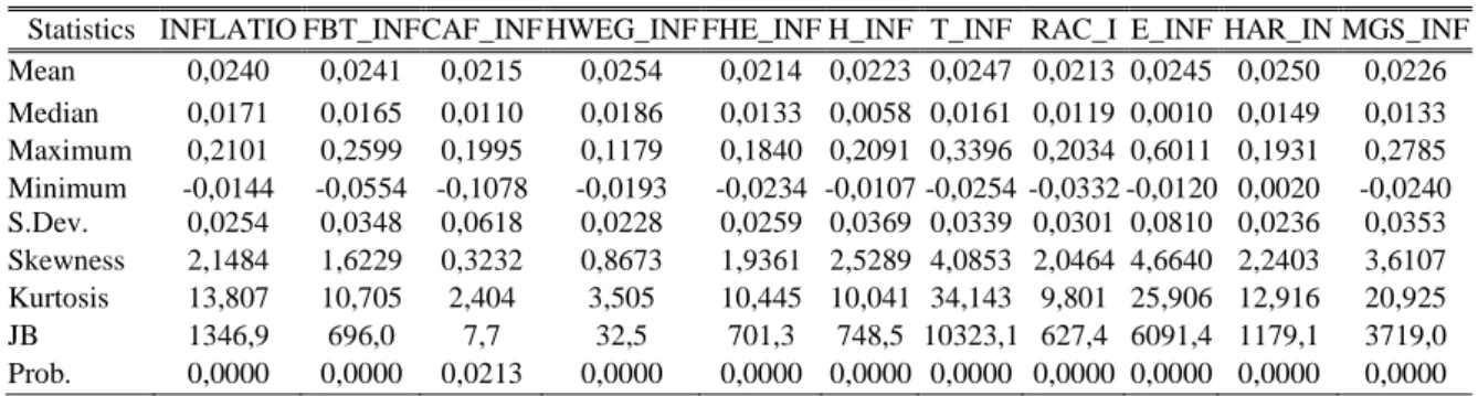
The descriptive statistics belonging to the variables involved in the study are presented in Table 1 and evaluate from statistical and economic point of view. It is seen that monthly mean inflation for the period of 1994:01-2013:12 is in the range of 2-2.5% and the main expenditure groups having the highest monthly mean inflation are housing (2.54%), restaurants (2.5%) and transportation (2.47%) and the main expenditure groups having the lowest monthly mean inflation are recreation (2.13%), furnishings (2.14%) and clothing (2.15%). The positiveness of the mean of the series indicates that there was a general tendency of increase in each of these expenditure groups in the period under investigation.
Table 1: Descriptive Statistics of Both the Inflation and Its Main Expenditure Groups
Statistics INFLATIO N
FBT_INF CAF_INF HWEG_INF FHE_INF H_INF T_INF RAC_I N E_INF HAR_IN F MGS_INF Mean 0,0240 0,0241 0,0215 0,0254 0,0214 0,0223 0,0247 0,0213 0,0245 0,0250 0,0226 Median 0,0171 0,0165 0,0110 0,0186 0,0133 0,0058 0,0161 0,0119 0,0010 0,0149 0,0133 Maximum 0,2101 0,2599 0,1995 0,1179 0,1840 0,2091 0,3396 0,2034 0,6011 0,1931 0,2785 Minimum -0,0144 -0,0554 -0,1078 -0,0193 -0,0234 -0,0107 -0,0254 -0,0332 -0,0120 0,0020 -0,0240 S.Dev. 0,0254 0,0348 0,0618 0,0228 0,0259 0,0369 0,0339 0,0301 0,0810 0,0236 0,0353 Skewness 2,1484 1,6229 0,3232 0,8673 1,9361 2,5289 4,0853 2,0464 4,6640 2,2403 3,6107 Kurtosis 13,807 10,705 2,404 3,505 10,445 10,041 34,143 9,801 25,906 12,916 20,925 JB 1346,9 696,0 7,7 32,5 701,3 748,5 10323,1 627,4 6091,4 1179,1 3719,0 Prob. 0,0000 0,0000 0,0213 0,0000 0,0000 0,0000 0,0000 0,0000 0,0000 0,0000 0,0000
When the standard deviation values that can give some insights into the volatility of the variables are examined, education (8.1%) and clothing (6.2%) come to the fore and except for housing and restaurants, all the groups have standard deviations quite higher than the mean. Based on the highness of this value showing the distribution of the series in relation to the mean, it is possible to claim that many values are higher than the mean value of all the series depending on a distribution quite far away from the means of all the series. At the same time, this may indicate that the series are under the influence of volatility. In a similar manner, the size of the difference between the minimum and maximum values of all the main expenditure groups supports the finding that price changes have high volatility. When the skewness values are examined, it is seen due to fact that positivity of skewness distribution of all the main expenditure groups are skewed towards right. This shows that unusual large shocks occurring in the series are more pervasive than small shocks and positive price changes are more likely than negative price changes. Moreover, lower median values than the means indicates the rightward skewness of the series. Jarque-Bera statistics do not confirm normal distribution of any series.
On the basis of all this information, in order to reveal whether the variables under investigation are stationary or not, ADF, PP and KPSS unit root test was conducted and the results are presented in Appendix 1. It is seen that those unit root tests have revealed different results from each other. As the obtained conflicting results indicate that there may be break in the series, whether any structural changes occurred in the inflation series in the period under investigation needs to be researched.
4.3. Conditional Volatility Estimates in Inflation and the Main Expenditure Groups Inflation Series With Structural Break At Mean and Mean of Variance Equation
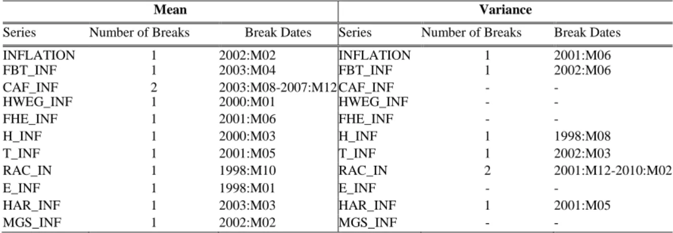
At that stage, BP method was employed to detect whether there are structural breaks in the mean and variance equation of inflation series.While conducting the application, as there might be heterogeneity in the error, the standard correction parameter was taken as 0.15 and the maximum number of breaks is allowed to be no more than 5 (Bai Perron, 2003a). While determining its location through the number of breaks, sequential testing was preferred and the results are presented in Table 2.
Table 2: The Results of Bai-Perron Structural Break Test for Inflation and the Main Expenditure Groups Inflation Series
GU J Sci, 29(2):343-363 (2016) / Pınar GÖKTAŞ, Ali ÇIMAT 347
Mean Variance
Series Number of Breaks Break Dates Series Number of Breaks Break Dates
INFLATION 1 2002:M02 INFLATION 1 2001:M06 FBT_INF 1 2003:M04 FBT_INF 1 2002:M06 CAF_INF 2 2003:M08-2007:M12 CAF_INF - - HWEG_INF 1 2000:M01 HWEG_INF - - FHE_INF 1 2001:M06 FHE_INF - - H_INF 1 2000:M03 H_INF 1 1998:M08 T_INF 1 2001:M05 T_INF 1 2002:M03 RAC_IN 1 1998:M10 RAC_IN 2 2001:M12-2010:M02 E_INF 1 1998:M01 E_INF - - HAR_INF 1 2003:M03 HAR_INF 1 2001:M05 MGS_INF 1 2002:M02 MGS_INF - -
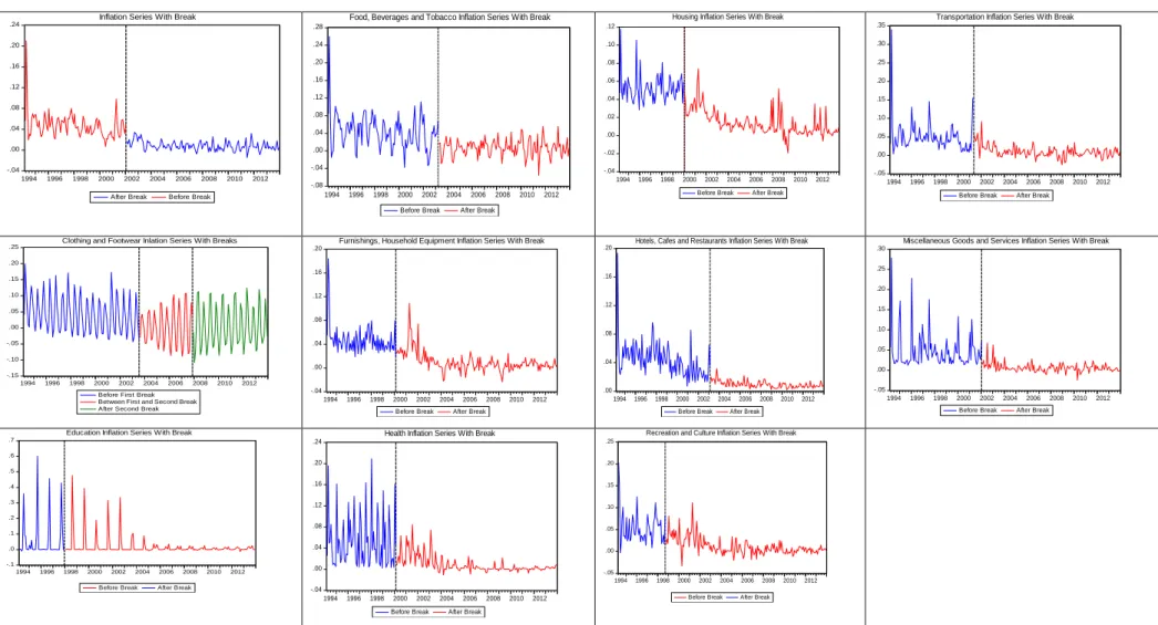
It is known that the Turkish economy has been deeply affected from crises, internal dynamics, conjectural changes in the world and has undergone many structural changes. This is clear in Tab. 2, which shows at least one break experienced in mean by all the indicators. Moreover, graphical representation of these breaks was displayed in Figure 1. For a variable experiencing breaks in its mean, it is usual to experience breaks in its error variance. In addition to this, not each inflation series experiencing a break in its mean experienced a break in the variance, only in the error variance of inflation and 5 different main expenditure groups, breaks were detected.
When the developments that may have changed the structure of the series are examined, the date 2001 is seen to be a turning point in terms of the implementation of monetary and fiscal policies. Moreover, these break periods indicate years considered to be turning points of the Turkish economy and some crisis periods. This finding supports that in Turkey, price changes have undergone important transformation and this mostly happened in crisis periods. These detected breaks need to be taken into consideration in volatility forecasts for inflation series.
In this first stage, the displays of the mean equations with the breaks are presented in Appendix 2 including
seasonal term in order to remove the seasonality effect. Furthermore, whether the errors of these mean equations are under the influence of stationarity and/or ARCH effect was investigated and the obtained results are presented in Appendix 3. As a result of the autocorrelation test administered, it was found that though all the residuals are stationary, they are under the influence of ARCH.
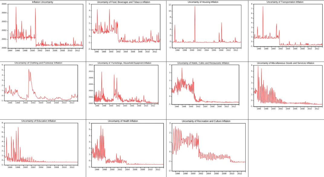
In the second stage, for each main expenditure group inflation, model searching was performed over all the uncertainty series obtained through ARCH, GARCH, EGARCH and TGARCH volatility forecasting models satisfying the model requirements. Thus, the main expenditure group volatility forecasts explaining inflation uncertainty in the modeling were preferred and the models having these characteristics are presented in Table 3 and their graphical display is presented in Figure 2.
In addition, in the suitable lag length of ARCH-LM test of all the models, it is seen that there is no ARCH effect remained in the residuals. This confirms that the models best filter the ARCH effect in the series and reflect in its own model. Furthermore, as a result of autocorrelation tests, stationarity of model residuals was detected and this clearly demonstrates the suitability of the models.
Table 3: The Most Representative Uncertainty Models Detected for Inflation and the Main Expenditure Groups Inflation
Series
Variables ARCH-LM(1) Stationarity of Residuals(2) Selected Model
INFLATION 0.212247 (0.6454) Stationary EGARCH(1,1)
FBT_INF 12.15273 (0.1445) Stationary EGARCH(1,0)
CAF_INF 2.782834 (0.7334) Stationary GARCH (1,1)
HWEG_INF 0.818772 (0.3655) Stationary EGARCH (2,0)
FHE_INF 2.876571 (0.0899) Stationary EGARCH (2,5)
H_INF 0.194895 (0.6589) Stationary EGARCH(2,5)
T_INF 0.048214 (0.9762) Stationary EGARCH(1,0)
RAC_INF 0.428466 (0.9997) Stationary EGARCH (1,5)
E_INF 2.876227 (0.7191) Stationary EGARCH (0,6)
MGS_INF 0.055199 (0.8143) Stationary EGARCH (4,5) (1
) Values between brackets represent the significant p level.
(2)
Stationarity of selected the model residuals has been diagnosed using ADF, PP and KPSS unit root tests with 5% significance level.
GU J Sci, 29(2):343-363 (2016) / Pınar GÖKTAŞ, Ali ÇIMAT 349 -.04 .00 .04 .08 .12 .16 .20 .24 1994 1996 1998 2000 2002 2004 2006 2008 2010 2012
After Break Before Break Inflation Series With Break
Figure 1: The Graphical Representations For Each Main Expenditure Group with Specification of Break Points. -.08 -.04 .00 .04 .08 .12 .16 .20 .24 .28 1994 1996 1998 2000 2002 2004 2006 2008 2010 2012 Before Break After Break
Food, Beverages and Tobacco Inflation Series With Break
-.04 -.02 .00 .02 .04 .06 .08 .10 .12 1994 1996 1998 2000 2002 2004 2006 2008 2010 2012 Before Break After Break Housing Inflation Series With Break
-.05 .00 .05 .10 .15 .20 .25 .30 .35 1994 1996 1998 2000 2002 2004 2006 2008 2010 2012 Before Break After Break
Transportation Inflation Series With Break
-.15 -.10 -.05 .00 .05 .10 .15 .20 .25 1994 1996 1998 2000 2002 2004 2006 2008 2010 2012
Before First Break Between First and Second Break After Second Break
Clothing and Footwear Inlation Series With Breaks
-.04 .00 .04 .08 .12 .16 .20 1994 1996 1998 2000 2002 2004 2006 2008 2010 2012 Before Break After Break
Furnishings, Household Equipment Inflation Series With Break
.00 .04 .08 .12 .16 .20 1994 1996 1998 2000 2002 2004 2006 2008 2010 2012 Before Break After Break
Hotels, Cafes and Restaurants Inflation Series With Break
-.05 .00 .05 .10 .15 .20 .25 .30 1994 1996 1998 2000 2002 2004 2006 2008 2010 2012
Before Break After Break
Miscellaneous Goods and Services Inflation Series With Break
-.1 .0 .1 .2 .3 .4 .5 .6 .7 1994 1996 1998 2000 2002 2004 2006 2008 2010 2012
Before Break After Break
Education Inflation Series With Break
-.04 .00 .04 .08 .12 .16 .20 .24 1994 1996 1998 2000 2002 2004 2006 2008 2010 2012 Before Break After Break
Health Inflation Series With Break
-.05 .00 .05 .10 .15 .20 .25 1994 1996 1998 2000 2002 2004 2006 2008 2010 2012
Before Break After Break
Figure 2: Graphical Representations of Inflation Uncertainty and Uncertainty of Each Main Expenditure Groups Series .0000 .0001 .0002 .0003 .0004 .0005 1994 1996 1998 2000 2002 2004 2006 2008 2010 2012 Inflation Uncertainty -2 -1 0 1 2 3 4 5 1996 1998 2000 2002 2004 2006 2008 2010 2012 Uncertainty of Food, Beverages and Tobacco Inflation
-2 0 2 4 6 8 10 12 1996 1998 2000 2002 2004 2006 2008 2010 2012 Uncertainty of Housing Inflation
-1 0 1 2 3 4 5 6 7 8 1996 1998 2000 2002 2004 2006 2008 2010 2012 Uncertainty of Transportation Inflation
-1 0 1 2 3 4 5 6 1996 1998 2000 2002 2004 2006 2008 2010 2012
Uncertainty of Clothing and Footwear Inflation
.0000 .0002 .0004 .0006 .0008 .0010 .0012 1996 1998 2000 2002 2004 2006 2008 2010 2012
Uncertainty of Furnishings, Household Equipment Inflation
-1 0 1 2 3 4 1996 1998 2000 2002 2004 2006 2008 2010 2012 Uncertainty of Hotels, Cafes and Restaurants Inflation
-1 0 1 2 3 4 5 6 1996 1998 2000 2002 2004 2006 2008 2010 2012 Uncertainty of Miscellaneous Goods and Services Inflation
-1 0 1 2 3 4 5 6 7 8 1996 1998 2000 2002 2004 2006 2008 2010 2012 Uncertainty of Education Inflation
-1 0 1 2 3 4 5 6 1996 1998 2000 2002 2004 2006 2008 2010 2012 Uncertainty of Health Inflation
-2 -1 0 1 2 3 1996 1998 2000 2002 2004 2006 2008 2010 2012 Uncertainty of Recreation and Culture Inflation
GU J Sci, 29(2):343-363 (2016) / Pınar GÖKTAŞ, Ali ÇIMAT 351
4.5. Determining Relative Importance of Main Expenditure Groups Uncertainties on Inflation Uncertainty
In the current study, inflation uncertainty series and 10 main expenditure groups uncertainties series were used
as the dependent variable being and the independent
variables being obtained using
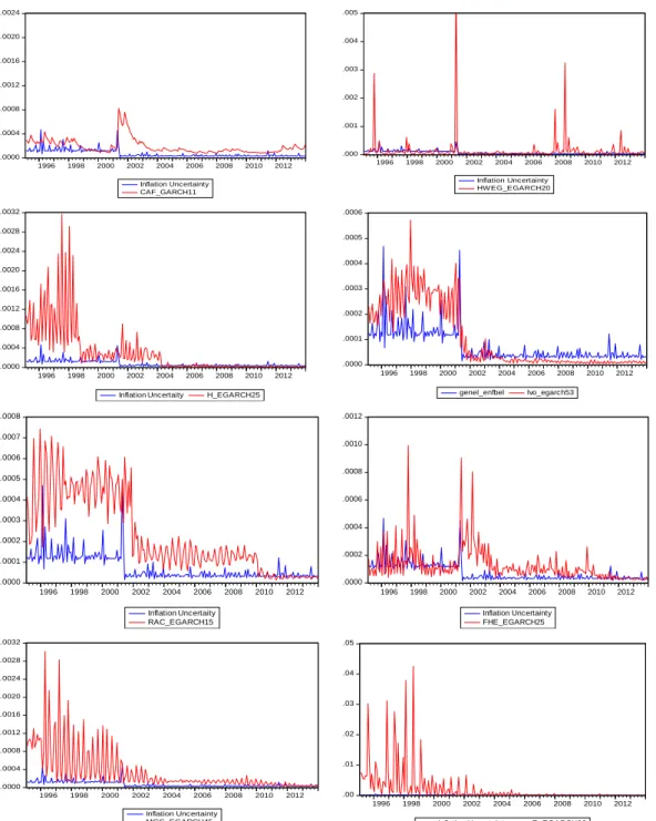
volatility forecasting models with structural break. Their names and definitions are presented in Appendix 4 and graphical display of plotting of inflation
uncertainty with the uncertainty for each of the main expenditure groups is presented in Figure 3. ARDL approach is also explained considering the number of these variables to preserve the integrity of information. As inflation is a value found through the combination of these expenditure groups, it can be argued that inflation uncertainty is the function of uncertainties experienced in these groups. In order to reveal the uncertainty of the main expenditure groups having the greatest effect on
the inflation uncertainty in the long run;
(5) Econometric display of the model can be expressed as below;
𝑌𝑡= 𝛾0+ 𝛾1𝑋1𝑡+ 𝛾2𝑋2𝑡+ 𝛾3𝑋3𝑡+ 𝛾4𝑋4𝑡+ 𝛾5𝑋5𝑡+ 𝛾6𝑋6𝑡+ 𝛾7𝑋7𝑡+ 𝛾8𝑋8𝑡+ 𝛾9𝑋9𝑡+ 𝛾10𝑋10𝑡+ 𝜀𝑡 (6)
When the series are in a co-integration relationship, the long run relationship between the variables can be revealed through the co-integration model obtained
without administering differentiation accordingly
without loss of any information. The long run coefficients at the same time show the weights of the uncertainties belonging to the main expenditure groups’ inflations within the inflation uncertainty here. However, for the order of importance (relative weights) of the variables involved in the co-integration equation showing that the series act simultaneously, all the variables in the regression (dependent and independent) should be standardized and then the regression should be reestimated with the standardized variables. As known, it is very simple to evaluate the relative importance of two independent variables measured with the same units on the y dependent variable. In the comparisons made, the one whose absolute regression coefficient is higher is considered to be more important. However, in practice and applications, the measurement units of the explanatory variables are not the same and
this makes it difficult to determine the relative weight order of the explanatory variables with ordinary regression coefficients. In order to deal with this problem, the variables are standardized and moved to the same unit measurement.
In this regard, the obtained standardized coefficients allow us make comparisons among the relative impacts of the independent variables on the dependent variable (Y) without relying on measurement units. They also provide the relative weights of each explanatory variable; namely, their partial contributions to unit change taking place in the dependent variable. At the same time, by using standardized coefficients, the contribution of each variable can be compared with the contributions of the other variables (Greene and D’Olivera, 2005). Therefore, in the current study, the co-integration equation was estimated over the standardized variables and the main expenditure group uncertainty having the greatest effect on inflation uncertainty was calculated with this method.
.0000 .0004 .0008 .0012 .0016 .0020 .0024 1996 1998 2000 2002 2004 2006 2008 2010 2012
Inflation Uncertainty T_EGARCH10
.0000 .0004 .0008 .0012 .0016 .0020 .0024 1996 1998 2000 2002 2004 2006 2008 2010 2012 Inflation Uncertinty FBT_EGARCH10
Figure 3: Plotting of Inflation Uncertainty with the Uncertainty For Each of The Main Expenditure Groups
4.5.1. Investigation of the co-integration relationship between the variables
ARDL methodology is performed across the stages presented below. In its basic form, ARDL model is as follows; .0000 .0004 .0008 .0012 .0016 .0020 .0024 1996 1998 2000 2002 2004 2006 2008 2010 2012 Inflation Uncertainty CAF_GARCH11 .000 .001 .002 .003 .004 .005 1996 1998 2000 2002 2004 2006 2008 2010 2012 Inflation Uncertainty HW EG_EGARCH20 .0000 .0004 .0008 .0012 .0016 .0020 .0024 .0028 .0032 1996 1998 2000 2002 2004 2006 2008 2010 2012
Inflation Uncertaity H_EGARCH25
.0000 .0001 .0002 .0003 .0004 .0005 .0006 1996 1998 2000 2002 2004 2006 2008 2010 2012 genel_enfbel lvo_egarch53 .0000 .0001 .0002 .0003 .0004 .0005 .0006 .0007 .0008 1996 1998 2000 2002 2004 2006 2008 2010 2012 Inflation Uncertaity RAC_EGARCH15 .0000 .0002 .0004 .0006 .0008 .0010 .0012 1996 1998 2000 2002 2004 2006 2008 2010 2012 Inflation Uncertainty FHE_EGARCH25 .0000 .0004 .0008 .0012 .0016 .0020 .0024 .0028 .0032 1996 1998 2000 2002 2004 2006 2008 2010 2012 Inflation Uncertainty MGS_EGARCH45 .00 .01 .02 .03 .04 .05 1996 1998 2000 2002 2004 2006 2008 2010 2012
GU J Sci, 29(2):343-363 (2016) / Pınar GÖKTAŞ, Ali ÇIMAT 353 𝑌𝑡= 𝜑 + ∑ 𝛾0𝑖𝑌𝑡−𝑖 𝑝 𝑖=1 + ∑ 𝛾1𝑖𝑋1𝑡−𝑖 𝑞1 𝑖=0 + ∑ 𝛾2𝑖𝑋2𝑡−𝑖 𝑞2 𝑖=0 + ∑ 𝛾3𝑖𝑋3𝑡−𝑖 𝑞3 𝑖=0 + ∑ 𝛾4𝑖𝑋4𝑡−𝑖 𝑞4 𝑖=0 + ∑ 𝛾5𝑖𝑋5𝑡−𝑖 𝑞5 𝑖=0 + ∑ 𝛾6𝑖𝑋6𝑡−𝑖 𝑞6 𝑖=0 + ∑ 𝛾7𝑖𝑋7𝑡−𝑖 𝑞7 𝑖=0 + ∑ 𝛾8𝑖𝑋8𝑡−𝑖 𝑞8 𝑖=0 + ∑ 𝛾9𝑖𝑋9𝑡−𝑖 𝑞9 𝑖=0 + ∑ 𝛾10𝑖𝑋10𝑡−𝑖 𝑞10 𝑖=0 + 𝜀𝑡 (7)
since the lag of the dependent variable is added to the first part of the model, it represents autogressive term and successive lags of the independent variable
in the second part represent distributed lag and represents white noise error term.
As known, though the bound test approach allows the series to be integrated at different levels, as it is based on the assumption that the variables are I(0) and I(1) and when the variables have greater integration level order, the t and F statistics in Pesaran et al. (2001) become invalid. Thus, in order to test the constraint, unit root tests were implemented and the obtained
results are presented in Appendix 5.It can be seen that
while some of the series are stationary at the level, some others are not stationary and when the first difference of all is considered, they become stationary. In such cases, co-integration analysis is suggested to prevent the problem of losing the long run relationship when the first differences are used (Gujarati, 2004).
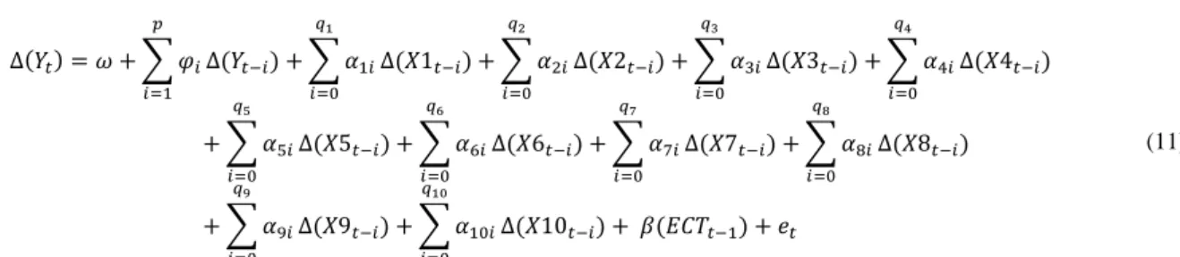
For the variables between which long run relationship is investigated, when the Unrestricted Error Correction
Model appearance in the
Eq. 8 is considered; ∆(𝑌𝑡) = 𝜔 + ∑ 𝜑𝑖 𝑝 𝑖=1 ∆(𝑌𝑡−𝑖) + ∑ 𝛼1𝑖 𝑞1 𝑖=0 ∆(𝑋1𝑡−𝑖) + ∑ 𝛼2𝑖 𝑞2 𝑖=0 ∆(𝑋2𝑡−𝑖) + ∑ 𝛼3𝑖 𝑞3 𝑖=0 ∆(𝑋3𝑡−𝑖) + ∑ 𝛼4𝑖 𝑞4 𝑖=0 ∆(𝑋4𝑡−𝑖) + ∑ 𝛼5𝑖 𝑞5 𝑖=0 ∆(𝑋5𝑡−𝑖) + ∑ 𝛼6𝑖 𝑞6 𝑖=0 ∆(𝑋6𝑡−𝑖) + ∑ 𝛼7𝑖 𝑞7 𝑖=0 ∆(𝑋7𝑡−𝑖) + ∑ 𝛼8𝑖 𝑞8 𝑖=0 ∆(𝑋8𝑡−𝑖) + ∑ 𝛼9𝑖 𝑞9 𝑖=0 ∆(𝑋9𝑡−𝑖) + ∑ 𝛼10𝑖 𝑞10 𝑖=0 ∆(𝑋10𝑡−𝑖) + 𝛽0𝑌𝑡−1+ 𝛽1𝑋1𝑡−1+ 𝛽2𝑋2𝑡−1+ 𝛽3𝑋3𝑡−1 + 𝛽4𝑋4𝑡−1+ 𝛽5𝑋5𝑡−1+ 𝛽6𝑋6𝑡−1+ 𝛽7𝑋7𝑡−1+ 𝛽8𝑋8𝑡−1+ 𝛽9𝑋9𝑡−1+ 𝛽10𝑋10𝑡−1+ 𝜀𝑡 (8)
In the equation, “∆” represents difference operator, β0⋯β10 coefficients represent long run relationships
and the remaining terms represent short run dynamics.
Null hypothesis H0: β0=β1=…=β10=0 showing the
absence of co-integration is tested with F-test shown as 𝐹(Yt|X1, X2,……,X10) versus alternative hypothesis
H1:β0≠β1≠…≠β10≠0. For the dependent variable, in
the testing of H0: β0=0 ve
H1: β0≠0 hypothesis, t-test is run. The calculated test
statistics must be compared with the critical values presented in Pesaran (2001).
As the variables used in the study are monthly series, maximum lag length is considered as 12. In this case, in order to be able to find the suitable lag length, different regressions will be estimated. Selection of the suitable criteria can be performed by using SBC and AIC criteria. In this connection, to
determine the optimum lag lenght of the model presented in Eq. (5), every single model with SBC and AIC up to 12 lag lenght has been performed. As a result of the model searching, OLS estimates obtained from
ARDL resulted in model having
the lowest AIC and SBC values are presented in Appendix 6.
For ARDL bound test approach, by using the coefficients in Table 5 must be tested. As known, if both of the hypotheses are rejected, then it can be claimed that the independent variables have a co-integration relationship with the dependent variable in the long run. For the testing of the first established hypothesis, Wald t statistics and for the second hypothesis, Wald F statistics must be calculated. The calculated test statistics are compared with the critical values presented in Pesaran (2001).
Table 5: ARDL Bound Test Co-integration Results
Hypothesis (2) k(1) Test statistic Lower Bound I(0)
(3)
Upper Bound I(1)(4)
1 10 -9.151678 -3.43 -2.86 -2.57 -5.68 -5.03 -4.69
2 10 9.840998 2.54 2.06 1.83 3.86 3.24 2.94
Note: (1) “k” represents (The number of parameters-1)
(2)
Critical values for the calculated t statistics of the first hypothesis have been obtained from the study of Pesaran (2001), page 303 of Table CII(iii) for the Case III and Critical values for the calculated F statistics of the second hypothesis have also been obtained from the study of Pesaran (2001), page 300 of Table CI(iii) for the Case III
(3, 4)
The percentage results represent the significance levels.
According to Wald t or F statistical values, both in the first and the second hypotheses, it is seen that the null hypothesis was rejected. Thus, it was proved that there is a long run co-integration between the main expenditure group uncertainty series and inflation uncertainty and these variables are not independent from each other and act simultaneously.
When a cointegreation is detected between the variables, from the long run regression equation, which is the normalized version of the Eq. 4, the ARDL model can be given below;
(9) From Eq. 6, the obtained residual series with one-lag that is used as an error correction term (ECT) may be presented in Eq. 7.
ECTt-1=(Yt-1- θ0-θ1X1t-1-θ2X2t-1-θ3X3t-1-θ4X4t-1-θ5X5t-1-θ6X6t-1-θ7X7t-1-θ8X8t-1-θ9X9t-1-θ10X10t-1) (10)
Following the Eq. 7, the given term is incorporated into the short run ARDL model as follows:
∆(𝑌𝑡) = 𝜔 + ∑ 𝜑𝑖 𝑝 𝑖=1 ∆(𝑌𝑡−𝑖) + ∑ 𝛼1𝑖 𝑞1 𝑖=0 ∆(𝑋1𝑡−𝑖) + ∑ 𝛼2𝑖 𝑞2 𝑖=0 ∆(𝑋2𝑡−𝑖) + ∑ 𝛼3𝑖 𝑞3 𝑖=0 ∆(𝑋3𝑡−𝑖) + ∑ 𝛼4𝑖 𝑞4 𝑖=0 ∆(𝑋4𝑡−𝑖) + ∑ 𝛼5𝑖 𝑞5 𝑖=0 ∆(𝑋5𝑡−𝑖) + ∑ 𝛼6𝑖 𝑞6 𝑖=0 ∆(𝑋6𝑡−𝑖) + ∑ 𝛼7𝑖 𝑞7 𝑖=0 ∆(𝑋7𝑡−𝑖) + ∑ 𝛼8𝑖 𝑞8 𝑖=0 ∆(𝑋8𝑡−𝑖) + ∑ 𝛼9𝑖 𝑞9 𝑖=0 ∆(𝑋9𝑡−𝑖) + ∑ 𝛼10𝑖 𝑞10 𝑖=0 ∆(𝑋10𝑡−𝑖) + 𝛽(𝐸𝐶𝑇𝑡−1) + 𝑒𝑡 (11)
In light of the above, as a result of model searching conducted by using AIC and SBC information criteria on the Eq. (7), ARDL(2,0,0,0,0,0,0,1,0,0,0) was obtained. The estimated results of the model are shown in Appendix 7. By including one lag of the residuals of
this model into the Eq. (8), the re-estimation was conducted. After normalization was administered to the model, the obtained long run co-integration results are presented in Table 6.
Table 6: Parameter Estimates of Long Run Co-integration Equation
Dependent Variable
Variable Coefficient Standardized Coefficient Test Statistic P-value
0.0000108 --- 2.412396 0.0167 0.1623479 0.3558991 7.014110 0.0000 -0.1704214 -0.3253826 -7.912309 0.0000 0.0119463 0.0841174 2.244549 0.0258 0.0835068 0.1668403 2.503045 0.0131 0.0354218 0.2725039 9.526206 0.0000 0.1269189 0.4512709 8.889989 0.0000 0.0291217 0.2290639 9.361180 0.0001 -0.0691100 -0.2043759 -3.599195 0.0004 0.0391511 0.0777966 2.182651 0.0302
GU J Sci, 29(2):343-363 (2016) / Pınar GÖKTAŞ, Ali ÇIMAT 355
0.0003455 0.0303646 0.844175 0.3995
Short-Term Error Correction Term
-0.854599 (0.0000)
It is seen that the error correction term (ECT) coefficient in the model is negative and significant as expected. As known, a coefficient of this term shows how much of the volatility occurring in the short run will reach equilibrium in the long run. It indicates that nearly 85% of the uncertainty that will be experienced in the long run will reach equilibrium one period later. When the coefficients belonging to the main expenditure group inflation uncertainties are examined, it is notable that the long run coefficients of the “clothing and footwear” and “recreation and culture” sub-groups are negative. This finding shows that customers’ reactions to the price increases and decreases in these groups, which are not considered to be primary needs by the customers, are in the reverse direction in response to price changes in the economy.
For instance, when uncertainty increases in the inflation, the price changes in the expenditure groups viewed to be less important by consumers seem to decrease. Uncertainties experienced in the other expenditure groups move in the same direction with inflation uncertainty.
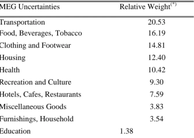
After this stage, relative weights of the main expenditure groups on inflation uncertainty that is the main focus of the study will be determined. Following the standardization of all the variables (dependent and independent variables), regression model was estimated with the standardized variables. In this regard, the main expenditure groups and uncertainty relative weights calculated for the period of 1994-2013 are reported in Table 7.
Table 7: Relative Weights of the Main Expenditure Groups Uncertainties on Inflation Uncertainty For The Period of
1994-2013
MEG Uncertainties Relative Weight(*)
Transportation 20.53
Food, Beverages, Tobacco 16.19
Clothing and Footwear 14.81
Housing 12.40
Health 10.42
Recreation and Culture 9.30
Hotels, Cafes, Restaurants 7.59
Miscellaneous Goods 3.83
Furnishings, Household 3.54
Education 1.38
(*)
Relative weights are obtained from the absolute standardized coefficients as contribution to uncertainty of inflation in percentages.
When the weights of expenditure groups uncertainties between the years of 1994 and 2013 are considered, it is seen that the “transportation” has the highest relative importance on price instability different from the expectation. The uncertainty of “food, beverages, tobacco” main expenditure group is in the second order in terms of relative importance. Besides, it is clearly observed from Figure 3 that in the long run, price fluctuations in the sectors moving most obviously together with inflation uncertainty are in fact “transportation” and “food, beverage and tobacco” uncertainties.
5. RESULTS AND FINDINGS
Changes taking place in price movements should be comprehensively addressed to enhance the efficiency
and permanency of the economic policy to be implemented in disinflation. In addition to this, in the international literature, the phenomenon of inflation is generally explained over the general level of prices and mostly the changes taking place at lower levels are overlooked.
In Turkey, as the general level of prices, Consumer Price Index (CPI) is used and inflation is calculated on the basis of the value changes in this index. Therefore, CPI was used for the analysis of inflation uncertainty in the present study; however, while doing this, the measurements considering not only the price changes in CPI but also price fluctuations experienced in all the lower levels.
From the long run established by using the standardized uncertainty series determined to have co-integration between them through ARDL approach, relative weights of the main expenditure group inflation
uncertainties within inflation uncertainty were
determined. It was observed that long run inflation uncertainty and “clothing and footwear” and “recreation
and culture” sub-groups price uncertainties move in reverse direction and the uncertainties experienced in the other main expenditure group move in the same direction. Moreover, the average weight of the main group expenditure groups CPI in 1994-2013 is presented in Table 8.
Table 8: The Average Weight of The Main Group Expenditure Groups in CPI in 1994-2013
MEG Average Weight (*)
Food, Beverages, Tobacco 32.07
Housing 20.87
Transportation 11.30
Clothing and Footwear 8.57
Furnishings, Household 8.05
Miscellaneous Goods 6.88
Hotels, Cafes, Restaurants 4.64
Recreation and Culture 3.05
Health 2.63
Education 1.95
(*)
It states that average weight of main expenditure groups of CPI for the period of 1994-2013 in percentages. Source: Turkish Statistical Institute
The sectors having the highest mean weight in the investigated period and explaining nearly 64% of the index are food, beverage, tobacco, housing and transportation and these main groups are expected to have a strong effect on inflation. That is, in the last 20 years, consumers spend 64% of their expenditures on these groups.
On the other hand, within fluctuations seen in the general level of prices, the weight of these groups in inflation uncertainty corresponds to only 49.1% (See Tab. 7). Therefore, almost half of the price fluctuations experienced in the last twenty years have resulted from the volatilities in these three main expenditure groups. Moreover, in Figure 3, it is illustrated that there is a parallelism between one expenditure group uncertainty and inflation uncertainty. It is clearly seen that in the long run, price fluctuations in the sectors moving most obviously together with inflation uncertainty are in “transportation” and “food, beverage and tobacco”. In addition, the sector moving together most obviously with inflation uncertainty in the long run and giving the fastest response to changes in inflation uncertainty is transportation.
Thus, when the weight of an expenditure group is high on CPI; that is, it constitutes a great portion of the consumption pattern of a citizen and when some changes occur in this group that does not mean that it would create a change at the same ratio in general inflation.
In this regard, contribution to inflation and contribution to inflation uncertainty are different things. As stated
before, as most of the groups having greater weight in consumption are required and cannot be substituted, sensitivity to increasing prices is restricted due to reasons such as deeply-rooted consumption patterns. Therefore, price changes taking place in these groups do not lead to uncertainty as large as expected.
As known, in recent years, it has been emphasized by both CBRT and economic circles that high inflation figures have resulted from the negative direction of food prices and failure in achieving the inflation targets has been explained by the increases in food prices. However, the present study also revealed that this assumption made on the basis of the high ratio of foods in CPI may not be true. However, after 2001 Turkey has made a fair success in terms of price stability and managed to keep inflation below 10%. This is why the study should be reperformed for the period after 2002 to check if there is a difference in the sources of price instability.
In the meanwhile, one of the most outstanding outcomes of the current study is revelation of the relative importance of the transportation main expenditure group in price uncertainties. It has been ignored for years that oil prices have been a key role in affecting inflation. For CPI inflation, there is a direct relationship between changes in oil prices and inflation itself. Shocks occurring in oil prices speed up CPI inflation in proportion to the weight of automotive fuel within the CPI (Norman and Richards, 2012, p. 71). It is clear that liquid fuel which is itself a cost and the large consumption proportion of it has a significant role on price instability in developing countries like Turkey.
GU J Sci, 29(2):343-363 (2016) / Pınar GÖKTAŞ, Ali ÇIMAT 357
Moreover in most of non-oil producing countries such as Turkey, these developments become even more obvious.
As a conclusion, in countries like Turkey implementing inflation targeting and experiencing some difficulties in achieving the target, policies for solutions should be created considering price movements particularly in
sectors having relatively higher importance in price uncertainties.
CONFLICT OF INTERESTS
The authors declare that there is no conflict of interests
regarding the publication of this paper.
REFERENCES
[1] Antoshin, S. Berg, A. & Souto, M. (2008). Testing For Structural Breaks In Small Samples.
International Monetary Fund (IMF) Working Paper African Department, 75
[2] Bai, J. (1997). Estimating Multiple Breaks One At A Time. Econometric Theory, 13 (3), 315-352 [3] Bai, J., Perron, P. (1998). Estimating and Testing
Lineer Models With Multiple Structural Change.
Econometrica, 66 (1), 47-78
[4] Bai, J., Perron, P. (2003a). Computation and Analysis of Multiple Structural Change Models,
Journal of Applied Econometrics, 18, 1-22.
[5] Bai, J., Perron, P. (2003b). Critical Values For Multiple Structural Change Tests. Econometrics
Journal, 6, 72–78
[6] Bai, J., Perron, P. (2004). Multiple Structural
Change Models: A Simulation Analysis.
http://www.columbia.edu/~jb3064/papers/2006_M ultiple_structural_changes_models_a_simulation_a nalysis.pdf.
[7] Ball, L. (1992). Why Does Higher Inflation Raise Inflation Uncertainty? Journal of Monetary
Economics, 29(3), 371-388
[8] Banerjee, S. (2013). Essays on inflation volatility (Doctoral dissertation, University of Durham) [9] Banerjee, P. & A., Rahman, M. (2012). Carbon
Emissions and Environment: Evidences from Three Selected SAARC Countries. Southwest
Business and Economics, 1-13.
[10] Bollerslev, T. (2007). Glossary to ARCH (GARCH). Center for Research in Econometrics
Analysis of Time Series Research Paper
[11] Carare, A., Schaechter, A., Stone , M.ve Zelmer, M.(2002). Establishing Initial Conditions in Support of Inflation Targeting. IMF Working
Paper, 102
[12] Cukierman A. & Meltzer A.H. (1986). A Theory of Ambiguity, Credibility and Inflation Under
Discretion and Asymmetric Information.
Econometrica, 54( 5), 1099-1128
[13] Dickey, D. A. & W. A. Fuller (1981). Likelihood Ratio Statistics for Autoregressive Time Series with a Unit Root. Econometrica, 49 (4), 1057-1072 [14] Drakos, A.A., Kouretas, G.P. & Zarangas, L.P. (2010). Forecasting financial volatility of the Athens stock exchange daily returns: An application of the Asymmetric normal mixture GARCH model. International Journal of Finance
and Economics, 15, 331–350
[15] Endresz, M. V. (2004). Structural Breaks And Financial Risk Management. Magyar Nemzeti
Bank, MNB Working Paper, 11, 1-56
[16] Enders, W.& Sandler, T. (2005). After 9/11: Is It
All Different Now?. Journal of Conflict
Resolution, 49 (2), 259-277
[17] Engle, R. F. (1982). Autoregressive Conditional Heteroscedasticity with Estimates of the Variance of United Kingdom Inflation. Econometrica, 50
(4), 987-1007
[18] Engle, R.F. & Granger, C.W.J. (1987). Co-integration and Error Correction: Reprenetationi Estimation, And Testing. Econometrica, 55(2), 251-276
[19] Friedman, M. (1977). Nobel Lecture: Inflation and Unemployment. Journal of Political Economy,
85(3), 451-472
[20] Frimpong, J.M.& Oteng-Abayie, E.F. (2006). Bounds Testing Approach: An Examination of Foreign Direct Investment, Trade, and Growth Relationships. Munich Personel RePEc Archive
(MPRA), 352
[21] Greene, J. & D’Olivera, M. (2005), Learning to
use statistical tests in psychology, New York:
[22] Grier K.B. & Perry M.J. (1998). On Inflation and Inflation Uncertainty in the G7 Countries. Journal
of International Money and Finance, 17, 671-689
[23] Gujarati, D. N. (2004). Temel Ekonometri. (Ü. Şenesen ve G. Günlük Şenesen, Çev.). İstanbul: Literatür Yayınları.
[24] Hentschel, L. (1995). All In The Family Nesting Symmetric And Asymmetric GARCH Models.
Journal of Financial Economics, 39, 71-104
[25] Holland, A.S. (1995). Inflation and Uncertainty: Tests for Temporal Ordering. Journal of Money,
Credit and Banking, 27(3), 827-837
[26] Johansen, S. (1988). Statistical Analysis of Cointegration Vectors. Journal of Economic
Dynamics and Control, 12(2–3), 231–254
[27] Johansen, S. (1991). Estimation and Hypothesis Testing of Cointegration Vectors in Gaussian Vector Autoregressive Models. Econometrica,
59(6), 1551-1580
[28] Johansen, S. (1995). Identifying Restrictions of
Linear Equations With Applications To
Simultaneous Equations and Cointegration.
Journal of Econometrics, 69(1), 111–132
[29] Johansen, S. & Juselius, K. (1990). Maximum
Likelihood Estimation And Inference On
Cointegration – With Applcations To The Demand For Money. Oxford Bulletin Of Economics and
Statistics, 52(2), 169-210
[30] Kwiatkowski, D., Phillips, P.C.B., Schmidt,P. & Shin, Y. (1992): Testing the Null Hypothesis of Stationarity against the Alternative of a Unit Root. Journal of Econometrics, 54, 159-178.
[31] Larsen, E.R. (2004). Does the CPI Mirror Costs-ofLiving? Engel's Law Suggests Not in Norway.
Statistics Norway, Research Department, Discussion Papers, 368
[32] Laurenceson J. & Chai J. (2003). Financial reform
and economic development in China. Advance in
Chinese Economic Studies Series, Cheltenham, UK: Edward Elgar Publishing Limited
[33] Mankiw, N.G. (2006). Principles of
macroeconomics, Sixth Edition. United States of
America: Worth Publishers.
[34] Narayan, P.K.& Narayan, S. (2005). Estimating Income And Price Elasticities of Imports for Fiji in A Cointegration Framework. Economic Modelling
22, 423– 438
[35] Norman, D. & Richards, A. (2012). The Forecasting Performance of Single Equation Models of Inflation. Economic Record, 88(280), 64-78
[36] Omotosho, B.S. & Doguwa, S.I. (2013). Understanding the Dynamics of Inflation Volatility in Nigeria: A GARCH Perspective. CBN Journal
of Applied Statistics, 3(2), 51-74
[37] Pelipas, I. (2012). Multiple Structural Breaks And Inflation Persıstence in Belarus. Belarusian
Economic Research and Outreach Center, Working Paper Series, BEROC WP, 021
[38] Pesaran, M.H.& Shin, Y. (1998). An
autoregressive distributed lag modelling approach to cointegration analysis. S. Strom (Ed.),
Econometrics and Economic Theory in the 20th
Century: The Ragnar Frisch Centennial
Symposium (pp. 371-413). UK: Cambridge University Press.
[39] Pesaran, H.M.; Shin Y. & Smith R. (1999). Bounds Testing Approaches to the Analysis of Level Relationships. Journal Of Applied Econometrics,
16, 289-326
[40] Pesaran, M.H., Shin, Y. & Smith, R.J. (2001). Bounds Testing Approaches to the Analysis of
Level Relationships. Journal of Applied
Econometrics, 16 (3), 289-326
[41] Petursson, T.G. (2000). Exchange rate or inflation targeting in monetary policy? Monetary Bulletin, 1, 36-45
[42] Phillips, P.C.B. & Hansen, B.E. (1990). Statistical Inference in Instrumental Variables Regression with I(1) Processes. Review of Economic Studies,
57, 99-125
[43] Phillips , P.C.B., Perron, (1988). Testing For A in time Series Reggression. Biometrica, 75(2), 335-346
[44] Pourgerami, A. & Maskus, K.E. (1987). The Effects of Inflation on the Predictability of Price Changes in Latin America: Some Estimates and Policy Implications. World Development, 15(2), 287-290
[45] Shahbaz, M., Adnan, H. Q. M. & Kumar, T.A. (2012). Economic Growth, Energy Consumption, Financial Development, International Trade and CO2 Emissions in Indonesia. Munich Personel
RePEc Archive (MPRA), 43294
[46] Tsyplakov, A. (2010). The Links Between Inflation And Inflation Uncertainty At The Longer Horizon. Economics Education and Research
Consortium: Russia and CIS, Working Paper No10/09E
[47] Türkiye Cumhuriyet Merkez Bankası (2001). Türkiye’nin Güçlü Ekonomiye Geçiş Programı. [48] Türkiye Cumhuriyet Merkez Bankası, (2006).
GU J Sci, 29(2):343-363 (2016) / Pınar GÖKTAŞ, Ali ÇIMAT 359
[49] Zapodeanu, D., Cociuba, M.I. and Petris, S. (2014), The Inflation- Inflation Uncertainty Nexus In Romania. International Conference “Monetary,
Banking and Financial Issues in Central and Eastern EU Member Countries: How Can Central and Eastern EU Members Overcome the Current Economic Crisis?. Iaşi, Romania, 10-12 April
APPENDIX
Appendix 1: Unit Root Examination of the Inflation Series belonging to Inflation and the Main Expenditure Groups
(1994:01-2013:12)(1,2)
Method M INFLATION FBT_INF CAF_INF HWEG_INF FHE_INF H_INF T_INF RAC_IN E_INF HAR_INF MGS_INF
ADF) N -2.194 -2.470 -3.591 -2.198 -4.500 -1.799 -2.867 -2.776 -1.531 -2.419 -2.540 I -1.871 -2.677 -2.632 -2.620 -5.120 -1.199 -4.632 -3.130 -1.430 -2.889 -2.339 IT -7.911 -8.902 -1.623 -7.051 -9.289 -1.460 -9.862 -10.704 -2.625 -6.500 -13.904 PP) N -4.584 I -5.756 -6.809 -9.626 -3.152 -8.269 -9.017 -5.462 -4.304 -6.704 -10.050 -7.332 -5.871 -11.453 -2.706 -12.278 -10.106 -8.085 -11.985 -5.925 -10.110 -12.498 IT -9.831 -8.948 -8.530 -11.324 -10.612 -15.565 -12.309 -10.950 -15.265 -12.061 -14.163 KPSS I 2.012 2.178 0.496 1.886 1.735 2.185 1.885 1.880 1.391 1.912 2.024 IT 0.459 0.233 0.182 0.329 0.297 0.213 0.279 0.341 0.109 0.472 0.266 (1)
Bold values refers to existance of unit root.
(2) N, I and IT represent “None”, “Intercept” and “Intercept and Trend” components respectively.
Appendix 2: The Mean Equations with Structural Breaks of Inflation and Main Expenditure Groups Series
Dependent Var. Mean Equation
INFLATION
0.0169298993153*D1+0.460244976123*D1*INF(-1) +0.0935416263364*D1* INF(-5) +
0.444756240424*D2*INF(-1) + 0.129792604227*D2* INF(-5) + 0.0113324816663*@SEAS(1) + 0.00856340452899*@SEAS(4) - 0.00963173113866*@SEAS(6) + 0.0124226359211*@SEAS(9) + 0.0137850863729* @SEAS(10)
FBT_INF
0.016*D1 + 0.489*D1*FBT_INF(-1) - 0.282*D1*FBT_INF(-4) + 0.270*D1* FBT_INF(-5) + 0.006*D2 - 0.134*D2*FBT_INF(-4) - 0.190*D2*FBT_INF(-12) + 0.024*@SEAS(1) +0.0171* @SEAS(2) + 0.013*@SEAS(3) - 0.014*@SEAS(5) - 0.031*@SEAS(6) + 0.010*@SEAS(9) + 0.022*@SEAS(10) + 0.012*@SEAS(11)
CAF_INF
0.014*D1 + 0.170*D1*CAF_INF(-1) + 0.161*D1*CAF_INF(-4) + 0.197*D1*GV A_ENF(-5) - 0.169*D1*CAF_INF(-10) + 0.098*D1*CAF_INF(-11) + 0.256*D1* CAF_INF(-12) + 0.005* D2 + 0.563*D2*CAF_INF(-1) - 0.399*D2*CAF_INF(-2) - 0.321*D2*CAF_INF(-3) + 0.180* D2*CAF_INF4) - 0.229*D2*CAF_INF6) + 0.253*D2*CAF_INF7) + 0.288 *D2*GVA_ ENF (-11) - 0.203*D2*CAF_INF(-12) + 0.007*D3 +0.244*D3*CAF_INF(-1) - 0.374*D3*GVA _ENF(-2) + 0.197*D3*GV A_ENF(-3) - 0.321*D3*CAF_INF(-4) + 0.257*D3 *CAF_INF(-10) + 0.439*D3*G VA_ENF(-12) - 0.044*@SEAS(1) - 0.043*@SEAS(2) - 0.034*@SEAS(3) + 0.048* @SEAS(4) + 0.020*@SEAS(5) - 0.018*@SEAS(7) - 0.024*@ SEAS(8) +0.041*@ SEAS(10)
HWEG_INF
0.061*D1 - 0.176*D1*HWEG_INF3) - 0.195*D1*HWEG_INF8) + 0.089*D1*KS EG_ENF (-11) - 0.002*D2 + 0.392*D2*HWEG_INF(-1) + 0.173*D2*HWEG_INF(-4) + 0.202*D2* HWEG_INF(-6) + 0.012*@SEAS(1) + 0.005*@SEAS(6) + 0.005*@ SEAS(7) + 0.007*@SEAS(8) + 0.014*@SEAS(9) + 0.012*@SEAS(10) + 0.005*@SEAS(11)
FHE_INF
0.025*D1 - 0.312*D1*FHE_INF(-1) + 0.170*D1*FHE_INF(-2) + 0.212*D1* MO BILYA_ ENF(-3) + 0.322*D1*FHE_INF(-4) + 0.449*D2* MO BILYA_ENF(-1) + 0.207* D2* FHE_INF(-2) + 0.145*D2*FHE_INF(-9) + 0.0124*@SEAS(1) + 0.005*@SEAS(9) + 0.005*@SEAS(10)
T_INF
0.031*D1 + 0.473*D1*T_INF(-1) + 0.212*D1*T_INF(-3) - 0.253*D1*T_INF(-4)+0.185*D1 *U _ENF(-5) - 0.241*D1*T_INF(-6) - 0.078*D1*T_INF(-11) + 0.353*D2*T_INF(-1) + 0.178* D2* T_INF(-5) + 0.125*D2*T_INF(-9) + 0.019*@SEAS(1) + 0.009*@SEAS(4) + 0.010*@SEAS(7)
H_INF
0.0233*D1 - 0.279*D1*H_INF(-1) + 0.364*D1*H_INF(-6) + 0.278*D1*H_INF(-7) - 0.232* D1*H_INF(-9) + 0.362*D1*H_INF(-12) + 0.325*D2*H_INF(-1) - 0.156*D2*H_INF(-2) + 0.213*D2*H_INF(-3) + 0.132*D2*H_INF(-4) + 0.266*D2*H_INF(-6) - 0.195*D2*H_INF (-9) + 0.167*D2*H_INF(-12) + 0.0145*@SEAS(1) + 0.008*@SEAS(3) + 0.0010*@SEAS(4)
RAC_INF
0.065*D1 + 0.514*D1*RAC_INF(-1) - 0.234*D1*RAC_INF(-2) - 0.230*D1*RAC_INF(-4) +
0.176*D1*RAC_INF(-5) - 0.191*D1*RAC_INF(-6) - 0.160*D1*RAC_INF(-8) -
0.337*D1*RAC_INF(-10) + 0.274*D1*RAC_INF(-11) - 0.092*D1*RAC_INF(-12) +
0.344*D2*RAC_INF(-1) + 0.245*D2*RAC_INF(-4) + 0.148*D2* RAC_INF(-5) +
GU J Sci, 29(2):343-363 (2016) / Pınar GÖKTAŞ, Ali ÇIMAT 361
E_INF
0.242*D1 - 0.236*D1*E_INF(-1) - 0.370*D1*E_INF(-2) - 0.339*D1*E_INF(-3) -
0.388*D1*E_INF(-4) - 0.370*D1*E_INF(-5) - 0.362*D1*E_INF(-6) - 0.407*D1*E_INF(-7) - 0.344*D1*E_INF(-8) - 0.399*D1*E_INF(-9) - 0.328* D1*E_INF(-10) - 0.416*D1*E_INF(-11) + 0.248*D1*E_INF(-12) - 0.106*D2 *E_INF(-1) + 0.282*D2*E_INF(-11) + 0.499*D2*E_INF(-12) - 0.0419*@ SEAS(7) + 0.0302*@SEAS(8) + 0.051*@SEAS(9)
HAR_INF
0.223*D1*HAR_INF(-1) + 0.404*D1*HAR_INF(-3) + 0.136*D1*HAR_INF(-7) +
0.131*D1*HAR_INF(-11) + 0.637*D2*HAR_INF(-1) + 0.013*@SEAS(1) + 0.006* @SEAS(2) + 0.005*@SEAS(4) + 0.005*@SEAS(8) + 0.006*@SEAS(9) + 0.006* @SEAS(10)
MGS_INF 0.0353*D1 + 0.108*D1*MGS_INF(-12) + 0.267*D2*MGS_INF(-6) + 0.216* D2*MGS_INF(-9) +
0.033*@SEAS(1)
Appendix 3: Stationarity and ARCH Effect Diagnosis of the Residuals Obteained From Mean Equations of Inflation Itself
and Inflation From Expenditures Variables
Breusch-Godfrey
Serial Correlation LM Test Breusch-Pagan-Godfrey Heteroskedasticity Test
F-statistic Obs*R-squared F-statistic Obs*R-squared
FBT_INF 0.138188 (0.9974) 1.134861 (0.9972) 2.647475 (0.0045) 24.83254 (0.0057) CAF_INF 0.433048 (0.5112) 0.464932 (0.4953) 2.231025 (0.0078) 29.14966 (0.0100) HWEG_INF 0.431408 (0.9568) 6.749883 (0.9146) 2.177953 (0.0009) 56.75343 (0.0022) FHE_INF 0.085028 (0.3736) 0.091408 (0.3565) 2.198205 (0.0192) 20.92778 (0.0216) H_INF 1.656097 (0.1995) 1.661407 (0.1974) 3.068080 (0.0008) 30.83328 (0.0012) T_INF 1.812861 (0.1459) 5.148086 (0.1613) 7.448952 (0.0000) 82.18703 (0.0000) RAC_INF 1.034498 (0.3103) 1.039639 (0.3079) 3.326678 (0.0001) 38.33001 (0.0003) FBT_INF 0.397118 (0.6720) 0.179321 (0.5293) 2.012893 (0.0137) 30.18430 (0.0171) RAC_INF 0.651194 (0.4206) 0.648137 (0.4208) 4.191362 (0.0000) 40.10583 (0.0000) E_INF 2.843228 (0.0605) 6.095640 (0.0475) 5.938328 (0.0000) 80.08051 (0.0000) MGS_INF 1.637566 (0.1816) 4.979899 (0.1733) 4.656691 (0.0005) 21.63611 (0.0006) *
Values between brackets represent the significant p level..
Appendix 4 Definitions of Uncertainty Series to be Used in the Modeling of Inflation Uncertainty
Variable Names Description
Inflation Uncertainty Y
Uncertainty of Food, Beverages and Tobacco Inflation X1
Uncertainty of Clothing and Footwear Inflation X2
Uncertainty of Miscellaneous Goods and Services Inflation X3
Uncertainty of Hotels, Cafes and Restaurants Inflation X4
Uncertainty of Housing Inflation X5
Uncertainty of Transportation Inflation X6
Uncertainty of Health Inflation X7
Uncertainty of Recreation and Culture Inflation X8
Uncertainty of Furnishings, Household Equipment Inflation X9
Appendix 5: Unit Root Detection For the Inflation Uncertainty and The Uncertainty of Main Sub-Groups(1)
Method ADF PP KPSS
Variable Level DI(2) Düzey DI DI Decision
Y -1.9918 I(1) -11.047 I(0) 1.51445 I(1)
X1 -1.7778 I(1) -5.2389 I(0) 1.47829 I(1)
X2 -3.5473 I(0) -3.4918 I(0) 0.68516 I(1)
X3 -2.6266 I(1) -13.7496 I(0) 1.49149 I(1)
X4 -1.1551 I(1) -2.7606 I(1) 1.51407 I(1)
X5 -14.598 I(0) -14.6001 I(0) 0.066064 I(0)
X6 -2.1142 I(1) -7.0713 I(0) 1.51436 I(1)
X7 -1.7599 I(1) -11.1607 I(0) 1.39955 I(1)
X8 -1.0643 I(1) -4.2359 I(0) 1.6931 I(1)
X9 -2.612 I(1) -12.8693 I(0) 0.9351 I(1)
X10 -1.2908 I(1) -13.0916 I(0) 1.75658 I(1)
(1)
Bold values refer to existence of unit root.
(2) “DI” refers the degree of integration.
Appendix 6: The Results of Unrestricted Error Correction Model From ARDL (1,1,6,0,3,3,0,1,0,0,1)
Dependent Variable
Variable Coefficient St. Error t-statistic p-value
1.52E-05 5.06E-06 3.003666 0.0030 -0.266716 0.060367 -4.418204 0.0000 0.193240 0.022770 8.486507 0.0000 0.061676 0.024174 2.551360 0.0116 0.153193 0.048666 3.147859 0.0019 0.006866 0.048381 0.141920 0.8873 -0.023621 0.044709 -0.528325 0.5979 -0.066901 0.041555 -1.609952 0.1091 -0.129474 0.032770 -3.951051 0.0001 -0.099750 0.032667 -3.053558 0.0026 -0.082574 0.032672 -2.527353 0.0123 0.005547 0.005284 1.049938 0.2951 0.107413 0.050777 2.115368 0.0358 0.122278 0.065447 1.868352 0.0633 0.126543 0.062950 2.010217 0.0459 0.140320 0.050540 2.776398 0.0061 0.033386 0.003268 10.21492 0.0000
GU J Sci, 29(2):343-363 (2016) / Pınar GÖKTAŞ, Ali ÇIMAT 363 -0.013157 0.007402 -1.777498 0.0772 -0.020481 0.005928 -3.455112 0.0007 -0.018753 0.004205 -4.460271 0.0000 0.100189 0.014146 7.082700 0.0000 0.008502 0.005415 1.569896 0.1182 0.009537 0.005481 1.739913 0.0836 -0.032877 0.021724 -1.513370 0.1319 0.004197 0.017266 0.243073 0.8082 8.98E-05 0.000411 0.218812 0.8270 -0.000544 0.000374 -1.455296 0.1473 -0.970326 0.106027 -9.151678 0.0000 0.086155 0.034592 2.490628 0.0136 -0.080956 0.028931 -2.798262 0.0057 0.010765 0.007788 1.382164 0.1686 0.131180 0.049658 2.641659 0.0090 0.038277 0.009095 4.208751 0.0000 0.113761 0.019349 5.879378 0.0000 0.016417 0.008539 1.922515 0.0561 -0.039576 0.023778 -1.664412 0.0978 -0.018655 0.025378 -0.735090 0.4632 0.000797 0.000657 1.212895 0.2267
R-square 0.906851 Akaike İnformation Criterion -18.46312
Adjusted R-square 0.887914 Schwarz Bayesian Criterion -17.87695
St. Error of Reg. 2.19E-05 Durbin-Watson statistic 2.128172
F-statistic 47.88790 Probability(F-stat) 0.000000 Breusch-Godfrey Autocorrelation LM(2) Testi 6.382787 (0.0411) ARCH Heteroscedasticity test 0.003674 (0.9517) Breusch-Godfrey Autocorrelation LM(12) Testi 16.80622 (0.1570) Ramsey-Reset F(1,181) test 13.49654 (0.0003)
Appendix 7 The Estimated Results of ARDL(2,0,0,0,0,0,0,1,0,0,0) Model
Dependent Variable
Variable Coefficient Standard Error t-statistic p-value
1.04E-05 4.31E-06 2.412396 0.0167 -0.140160 0.039564 -3.542628 0.0005 0.179113 0.042725 4.192201 0.0000 0.156024 0.022244 7.014110 0.0000 -0.163783 0.020700 -7.912309 0.0000 0.011481 0.005115 2.244549 0.0258
0.080254 0.032063 2.503045 0.0131 0.034042 0.003574 9.526206 0.0000 0.121975 0.013720 8.889989 0.0000 0.013368 0.004542 2.943619 0.0036 0.015140 0.005473 2.766375 0.0062 -0.066418 0.018454 -3.599195 0.0004 0.037626 0.017239 2.182651 0.0302 0.000332 0.000394 0.844175 0.3995
R-square 0.852720 Akaike İnformation Criterion -18.25092
Adjusted R-square 0.843646 Schwarz Bayesian Criterion -18.03836
St. Error of Reg. 2.56E-05 Durbin-Watson istatistiği 1.925516
F-statistic 93.97287 Olasılık(F-istatistiği) 0.000000 Breusch-Godfrey Serisel Autocorrelation LM(2) Testi 3.692767 (0.1578) ARCH Heteroscedasticity testi 0.008354 (0.9272) Breusch-Godfrey Serisel Autocorrelation LM(12) Testi 8.640282 (0.7333) Ramsey-Reset F(1,210) test 15.72869 (0.0001)