The Relationship between Inflation and the Budget Deficit in Turkey Author(s): Kivilcim Metin
Source: Journal of Business & Economic Statistics, Vol. 16, No. 4 (Oct., 1998), pp. 412-422 Published by: American Statistical Association
Stable URL: http://www.jstor.org/stable/1392610 .
Accessed: 03/05/2011 18:24
Your use of the JSTOR archive indicates your acceptance of JSTOR's Terms and Conditions of Use, available at .
http://www.jstor.org/page/info/about/policies/terms.jsp. JSTOR's Terms and Conditions of Use provides, in part, that unless you have obtained prior permission, you may not download an entire issue of a journal or multiple copies of articles, and you may use content in the JSTOR archive only for your personal, non-commercial use.
Please contact the publisher regarding any further use of this work. Publisher contact information may be obtained at .
http://www.jstor.org/action/showPublisher?publisherCode=astata. .
Each copy of any part of a JSTOR transmission must contain the same copyright notice that appears on the screen or printed page of such transmission.
JSTOR is a not-for-profit service that helps scholars, researchers, and students discover, use, and build upon a wide range of content in a trusted digital archive. We use information technology and tools to increase productivity and facilitate new forms of scholarship. For more information about JSTOR, please contact [email protected].
American Statistical Association is collaborating with JSTOR to digitize, preserve and extend access to Journal of Business & Economic Statistics.
The
Relationship
Between
Inflation
and
the
Budget
Deficit
in
Turkey
Kivilcim METINDepartment of Economics, Bilkent University, Ankara, Turkey ([email protected])
This article analyzes the empirical relationship between inflation and the budget deficit for the Turkish economy by a multivariate cointegration analysis. A single-equation model shows that the scaled budget deficit (as well as income growth and debt monetization) significantly affects inflation in Turkey. The conditional model of inflation is constant, and it encompasses a previously estimated model.
KEY WORDS: Cointegration; Encompassing; Exogeneity; Turkish inflation.
An extensive literature has examined the relationship be- tween the budget deficit and inflation. At a theoretical level, Sargent and Wallace (1981) showed that under certain con- ditions, if the time paths of government spending and taxes are exogenous, bond-financed deficits are nonsustainable, and the central bank should eventually monetize the deficit. This will increase the money supply and inflation in the long run. These findings have subsequently been general- ized for the open economy case and for alternative forms of financing (see Scarth 1987; Langdana 1990).
The empirical relationship between the deficit and in- flation in developed countries has been studied in detail (see Hamburger and Zwick 1981; Dwyer 1982; Hein 1983; Ahking and Miller 1985; King and Plosser 1985; Protopa- padakis and Siegel 1987; Burdekin and Wohar 1990; Ho
1990). Empirical studies of developing countries include those of Dornbush and Fisher (1981), Bhalla (1981), Sid- diqui (1989), Choudhary and Parai (1991), Buiter and Pa- tel (1992), Dogas (1992), Sowa (1994), Hondroyiannis and Papapetrou (1994), and Metin (1995). These studies did not yield conclusive results on the relationship between the bud- get deficit and inflation, either in the short run or in the long run. Specifically, Hamburger and Zwick (1981) found that growth in Federal Reserve debt holdings exerted a signif- icant inflationary impact on the U.S. economy over 1961- 1982, yet a growth in nonmonetized debt had a negative short-run effect on inflation. Ahking and Miller (1985) mod- eled deficits, money growth, and inflation over 1950-1980 as a trivariate autoregressive process. They found govern- ment deficits to be inflationary in the 1950s and 1970s but not in the 1960s. Using a rational-expectations macro model of Peruvian inflation, Choudhary and Parai (1991) found that budget deficits, as well as the growth rate of money supply, have significant impacts on inflation. Similarly, Do- gas (1992) found that the public deficit affects inflation in Greece. Hondroyiannis and Papapetrou (1994) also found a relationship between the Greek government budget and price level. Using an error-correction model, Sowa (1994) found that inflation in Ghana is influenced more by output volatility than by monetary factors, both in the long run and in the short run.
For Turkey, Metin (1995) analyzed inflation using a gen- eral framework of sectoral relationships and found that fis-
cal expansion was a determining factor for inflation. The excess demand for money affected inflation positively, but only in the short run. On the other hand, imported infla- tion, the excess demand for goods, and the excess demand for assets in the capital markets had little or no effect on inflation. A key policy implication of Metin (1995) is that Turkish inflation could be reduced rapidly by eliminating the budget deficit.
The aforementioned general literature influences the cur- rent study, which builds directly on Metin (1995). The large public-sector budget deficits and the relatively high inflation in Turkey during the last four decades have sparked de- bate on their consequences for the Turkish economy. The main question is whether bond-financed deficits are infla- tionary or whether only monetized deficits are inflationary. To answer this question, this article investigates the rela- tionship between Turkish inflation and budget deficits over 1950-1987. Although the government shifted from mone- tizing the deficit to bond financing in the mid-1980s, the short annual sample on Treasury bonds precluded sorting out the effects of this alternative means of deficit financing. Therefore, I have used Metin's (1995) dataset for analyz- ing the relationship between inflation and the public-sector budget deficit, considering a closed-economy public-finance approach. The closed-economy assumption may appear re- strictive, but Metin (1995) showed the lack of external ef- fects in the determination of Turkish inflation. The empiri- cal analysis herein is of general interest because many other developing countries have experienced budget and inflation difficulties similar to those in Turkey.
Section 1 presents a historical background to the Turk- ish economy for 1950-1987, and Section 2 develops a the- oretical framework based on the public-finance approach. Section 3 tests for budget deficits and inflation being coin- tegrated (and finds that they are). Although weak exogene- ity does not appear valid, a parsimonious conditional model is still developed (Sec. 4). This model is empirically con- stant, whereas the corresponding marginal model is not, thus showing super exogeneity for dynamics parameters.
?
1998 American Statistical Association Journal of Business & Economic Statistics October 1998, Vol. 16, No. 4 412Metin: The Relationship Between Inflation and the Budget Deficit in Turkey 413
Additionally, the new conditional model encompasses the model of Metin (1995).
1. HISTORICAL BACKGROUND
This section presents a brief economic history of Turkey, focusing on inflation and budget financing.
From the 1950s until 1980, the Turkish government con- sistently followed a policy of import substitution, with pro- hibitions on imports of commodities. State economic en- terprises (SEE's) were established to produce agricultural commodities, several manufactured goods, and minerals. In the late 1950s, the Turkish economy experienced se- vere balance-of-payment difficulties and rising inflation. Ef- forts to control inflation consisted largely of price controls. Private-sector firms responded either by shutting down or by selling on the black market. SEE's, however, sold at of- ficial prices and experienced losses. As inflation increased, these losses reached enormous amounts. The losses were automatically financed by the credits extended by the Cen- tral Bank to the SEE's, resulting in high money growth (see Aktan 1964; Okyar 1965; Fry 1972, 1980; Krueger 1974, 1995; Onis and Riedel 1993).
In 1958, Turkey implemented a fairly typical Interna- tional Monetary Fund (IMF)-supported stabilization pro- gram, which improved the foreign-exchange situation and drastically reduced inflation. The most important compo- nent of the program was an increase in the prices of SEE goods, a component that was featured prominently in the 1970 and 1980 reforms as well. Raising those prices in 1958 resulted in an immediate and once-and-for-all increase in the price level, after which the reduced rate of expansion of Central Bank credits reduced inflation. Although infla- tion dropped from 25% in 1958 to less than 5% in 1959, real gross domestic product (which had been declining) started growing immediately due to the greater availability of im- ports.
Turkey was among the more rapidly growing developing countries during most of the 1960s, with an annual infla- tion rate of 5%-10%. The nominal exchange rate was kept constant after the 1958 devaluation. Investment spending increased and was financed mainly by foreign aid. In the late 1960s, foreign aid did not increase, but the rate of in- vestment spending was maintained. In addition, some dif- ficulties appeared in obtaining imports, creating visible re- straints on economic activity and growth.
Although inflation was rising at the time, the main reason for the 1970 devaluation was foreign-exchange difficulties. After the devaluation, export earnings increased sharply, and Turkish workers in Germany and other western Eu- ropean countries started remitting a significant amount of foreign exchange. Because there was no mechanism read- ily at hand for the Central Bank to sterilize these inflows, the money supply expanded rapidly and inflation increased, reaching an annual rate of 25% by 1973. In the early and the mid-1970s, the problem of the growing public-sector deficit also arose from the expenditure side. In particular, large salary increases were granted to civil servants, and substantial increases in transfer payments were made to
SEE's, which had financial deficits due to both increased wage costs and a rise in the rate of investment by the SEE's (see Onis and Riedel 1993). The growth of government spending during a boom in the mid-1970s led to rising bud- get deficits, for which the Central Bank provided a major part of the financing. The public sector borrowing require- ment (PSBR) was 4.3% of gross national product (GNP) in
1973, more than doubling to 10.7% in 1979.
Inflation reached about 100% in 1980, apparently fed by monetization of the public-sector deficit. Policy changes in the early 1980s were designed to shift Turkey's growth strategy away from import substitution and toward greater integration with the international market. The 1980 stabi- lization program attempted to deal with inflation by cre- ating greater efficiency in operating the SEE's, restrain- ing the growth of public expenditure, reducing subsidies, and attempting to improve revenue collection. Under the government's liberalization program, the financial perfor- mance of SEE's improved substantially. Unlike their per- formance during the previous decades, SEE's appeared to have contributed positively to the financial position of the central government in the 1980s. The government's restric- tive stance could not be fully maintained, however. The PSBR remained at about 6% of GNP during the first half of the 1980s and rose to 8.3% in 1987, the highest since 1980. Contributing factors included slow growth of rev- enues, a strong increase in budget transfers to loss-making SEE's, higher than planned wage and salary raises in the public sector, and an election. After 1980, policy reforms continued. Although inflation fell to approximately 35% in
1982, it started rising again and continued to be a problem throughout the 1980s.
2. THE ECONOMIC FRAMEWORK
This section summarizes the theoretical model underlying the empirical analysis. In a closed economy, it is assumed that all public debt takes the form of noninterest-bearing money. The public sector budget identity is then
G - T = AH (1)
or
G-T AH
= (2)
py PY '
where G is public-sector expenditures, T is public-sector revenues, Y is real income, P is the price level, and H is base money. In a steady-state growing economy, it follows that A(H*) =(H*) Q4H zP LY AH S - H* (Ap + Ay), (3) pY
where A is the difference operator; H*, Ap, and Ay are scaled base money (H/PY), inflation, and the growth rate of real income, respectively; and variables in lower case are in logarithms. It is assumed that the long-run income elas- ticity of the demand for money is unity. Then the simplified
414 Journal of Business & Economic Statistics, October 1998
2.0
2.1
Figure !. Consumer Price Index and Base Money: p = , h = 1/.4 PY1 .78 - 4.2B = c + - (5) -4.9 1950 1955 1969" 1965 197 1975 1989 985 1999
Figure 1. Consumer Price Index and Base Money: p , h =
budget constraint is
A(H*) _B - H* (Ap + Ay). (4) Solving (4) for Ap, I obtain the following relation:
Ap = c + 1B - Vb2Ay, (5) where B is the scaled budget deficit (G - T)/H, c is the constant term (interpretable as the inertial inflation rate), and V) and V2 are slope coefficients associated with the scaled deficit and income growth. Here, V1 and 'Q2 are equal coefficients with an opposite sign [see Phelps (1973), Anand and van Wijnbergen (1989), and Rodrik (1990) for theory and empirical analysis]. The remainder of this article empir- ically analyzes the relationship between the budget deficit, inflation, base money, and real income growth.
3. THE DATA, UNIT-ROOT TESTS, AND COINTEGRATION ANALYSIS
This section tests for unit roots in the series of in- terest (Sec. 3.1) and for cointegration between the series (Sec. 3.2).
6.3-
1.8.
1959 1955 1969 1965 1979 1975 1989 1985 1999
Figure 2. Revenues and Taxes: g = , t = --.
.12
-.04
1950 1955 1960 1965 1970 1975 1980 1985 1990
Figure 3. The Growth Rate of Real Income: Ay =
3.1 The Data and Unit-Root Tests
The data used are annual over 1950-1987. Budget expen- ditures (G) and budget revenues (T) are from the budget and final accounts, respectively [Turkish lira (TL) Billion]. The general budget deficit (G - T) is the primary deficit, which excludes interest payments (TL Billion). The budget deficit does not include the SEE's deficit. Because reliable statistics about SEE's deficits are available only after the second half of the 1970s, the general budget deficit is there- fore used as a proxy for the total deficit. The price level (P) is the consumer price index with base year 1980, Y is real GNP (TL 1980 Billion), and H is base money. The compo- nents of base money are currency in circulation, vault cash, legal reserves, and Central Bank sight deposits (TL Billion). The Appendix describes the data in greater detail.
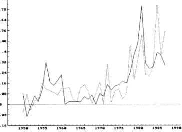
Figures 1--4 show (h, p), (t, g), Ay, and (Ap, B), respec- tively. Visually, all series appear at least I(1); the augmented Dickey-Fuller (1981) (ADF) test statistics in Table 1 sup- port the graphical explanation. p and h appear 1(2) (Fig. 1), and h* is I(1). Government expenditures (g) and revenues (t) also seem to be 1(2) (Fig. 2), but the scaled deficit B is clearly I(1). Ay is I(0) and, from its plot, looks like a
.64r- .56 .48
-.9.
1959 1955 1969 1965 1979 1975 1989 1985 1999
Figure 4. Inflation and the Rescaled Budget Deficit: zp = B =- -
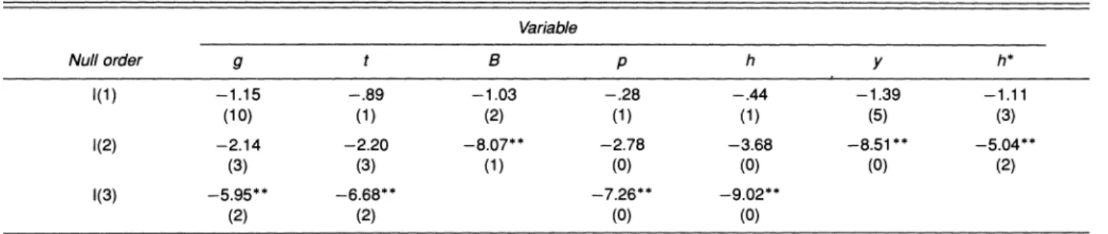
Metin: The Relationship Between Inflation and the Budget Deficit in Turkey 415 Table 1. Augmented Dickey-Fuller Test Statistics
Variable Null order g t B p h y h* I(1) -1.15 -.89 -1.03 -.28 -.44 -1.39 -1.11 (10) (1) (2) (1) (1) (5) (3) 1(2) -2.14 -2.20 -8.07** -2.78 -3.68 -8.51** -5.04** (3) (3) (1) (0) (0) (0) (2) I(3) -5.95** -6.68** -7.26** -9.02** (2) (2) (0) (0)
NOTE: For a given variable and null order, two values are reported. The first row is the t value, which is the ADF statistic, and the second row is the longest significant lag with significant t value. Five lags are allowed in each variable's ADF regression, but twelve lags are allowed for g and t. All regressions include a constant term and a trend. The sample is 1954-1987 (T = 34) if the variables are in their log levels (except B), 1955-1987 (T = 33) if they are in first differences, and 1956-1987 (T = 32) if variables are in second differences. The critical values are from MacKinnon (1991, table 1). Here and elsewhere in this article, ** and * denote rejection at the 1% and 5% critical values.
stationary heteroscedastic series (Fig. 3). Figure 4 captures the essence of the cointegration analysis: Both Ap and the scaled budget deficit B share the same upward trend over time.
3.2 System Cointegration Analysis
This subsection tests for cointegration among the se- ries (Ap, h*, B, Ay). I test for cointegration in a first-order vector autoregression (VAR), using the multivariate coin- tegration procedure of Johansen (1988) and Johansen and Juselius (1990). The VAR includes a constant term, a trend, and an impulse dummy (i1980). The impulse dummy rep- resents the structural change in the Turkish economy that took place in 1980. The constant and i 1980 enter the system unrestrictedly. The trend is restricted to lie in the cointegra- tion space because a quadratic deterministic trend in levels of economic variables is not usually a sensible long-run outcome (see Doornik and Hendry 1994). The cointegra- tion results are quite sensitive to the lag length of the VAR. Our choice of one lag is based on the Schwarz and Hannan- Quinn criteria, both of which pointed to a single lag. The estimation period is 1952-1987.
Table 2 summarizes the cointegration results. It includes the eigenvalues, the max and trace statistics, the standard- ized estimated feedback coefficients a and cointegrating vector p', and statistics for testing restrictions on a. The cointegration test statistics are corrected for sample size (see Reimers 1992), and they suggest three cointegrating vectors. The residual misspecification tests appear satisfac- tory. None of the equations exhibits autocorrelation, and the equations for B and Ay have nonnormal residuals.
Because I find three stationary relations, I need to identify the estimated cointegrating vectors before I interpret them. Assuming that Ay is trend stationary, the second row of the p3 is an inflation relation, and the third cointegrating vector is including just Ap and B, I test the identification of all cointegrating vectors. The expected /3' matrix will be
1 0 0 0
'= 01.*0 ,
0 ? 10,J
and implementing those identification restrictions leads to the restricted form /' and a matrix reported in Table 3. The likelihood ratio test statistic suggests that all three cointe-
grating vectors are identified X2(2) = 1.1559 [.5611] (see Johansen 1991, theorem 5.1).
From the standardized 3' eigenvectors, the first cointe- grating vector is the growth rate of real income. The second one is an inflation relation:
Ap = .58B + .35h*. (6) The public sector deficit B enters with a positive coefficient (.58), and scaled base money h* also has a positive coef-
Table 2. A Cointegration Analysis of {Ay, Ap, B, h*}
Eigenvalues .739 .662 .445 .085 Hypotheses r = 0 r < 1 r < 2 r < 3 Max statistic 40.4 32.5 17.7 2.7 95% critical value 27.1 21.0 14.1 3.8 Trace statistic 93.2 52.9 20.4 2.7 95% critical value 47.2 29.7 15.4 3.8 Standardized eigenvectors P' Variable Ay Ap B h* Trend 1 .188 -.124 -.088 .0006 -1.222 1 -2.515 -.769 .0128 -1.042 1.745 1 .009 -.0191 .125 .611 -.443 1 .0052
Standardized adjustment coefficients a
Ay -1.200 .097 .054 .006
Ap -.692 -.129 -.201 .042
B .079 .337 -.185 .071
h* -.016 .076 -.037 -.115
Weak exogeneity test statistics
Variable A y p B h* X2(5) 2.41 12.963 12.506 38.848 p value [.4911] [.0047]** [.0058]** [.000]** Diagnostic statistics Variable A y p B h* Normality X2(2) 11.35** .61 7.93* .24 ARCH 1 F(1, 25) 1.14 .58 .25 1.61 AR 1-2 F(2, 25) .86 1.29 1.27 1.44
NOTE: r is the hypothesized number of cointegrating vectors. The critical values for the cointe- gration tests are from Osterwald-Lenum (1992). The Jarque-Bera (1980) normality test statistic has a X2 distribution with 2 df under the null of normal errors. ARCH F(dfl, df2) refers to the test for ARCH errors, introduced by Engle (1982). The AR1 F(dfl, df2) is the test for residual
416 Journal of Business & Economic Statistics, October 1998 Table 3. A Restricted-Form Cointegration Analysis
Standardized eigenvectors /'
Variable Ay Ap B h* Trend
1.000 0.000 0.000 0.000 0.000
0.000 1.000 -0.585 -0.349 0.000
0.000 1.148 1.000 0.000 -0.012
Standardized adjustment coefficients a
Ay -1.348 -.024 -.038
Ap -.348 -.487 -.085
B -.157 .747 -.611
h* -.067 .162 -.134
Weak exogeneity test statistics Variable Ay Ap B
X2(6) 74.151 16.136 23.989
p value [.000] [.000] [.000]
ficient (.35). The third stationary relationship is between inflation and the scaled budget deficit.
The standardized a coefficients show that the main effect of the first cointegrating vector is on Ay. From the second column of a, feedback of the second cointegrating vector on both B and Ap is .75 and -.49, respectively. The third cointegrating vector primarily affects the scaled deficit B. Weak exogeneity for 3 can be tested using the Johansen (1992a,b) procedure. The results suggest that Ap, B, and h* cannot be assumed weakly exogenous for 0, but Ay can be (see Table 2). Weak exogeneity of the variables is also tested jointly with identification restriction and rejected for Ap, B, and Ay (see Table 3).
For inference, conditional models should have regressors that are weakly exogenous; see Engle, Hendry, and Richard (1983). In the context of cointegration, weak exogeneity means that inference about the cointegrating vector can be performed on the conditional model without loss of infor- mation relative to a system analysis. Even lacking weak exogeneity, single-equation modeling can proceed, treat- ing the system-based estimated cointegration coefficients as given; see Juselius (1992). Section 4 develops such a con- ditional model and examines its properties.
4. SINGLE-EQUATION MODELING
This section develops a parsimonious, conditional, single- equation model for inflation, in which inflation depends on the scaled budget deficit, the real growth rate of income, and scaled base money. Section 4.1 develops a parsimonious conditional model from a general autoregressive distributed lag and shows the constancy of this conditional model. Sec- tion 4.2 estimates some marginal equations and tests their constancy. Finally, Section 4.3 compares the model esti- mated by Metin (1995) with the conditional model devel- oped in this article, using the standard encompassing frame- work.
4.1 Single-Equation Analysis and the Constancy of a Conditional Model
Because weak exogeneity does not appear valid (except
for Ay), Juselius's (1992) approach is used for single- equation modeling. Recalling the cointegration analysis in the previous Section 3.2, a single inflation equation is con- structed. The inflation model includes the error-correction terms (ECM's) obtained from the earlier cointegration anal- ysis. The first ECM (CI2) is constructed using Equation (6), and the second ECM (CI3) is obtained from the third row of the f' matrix given in Table 3. Then the general ECM model involves A2p, AB, Ay (because it is stationary), Ah*, their lags, and the lagged ECM's. Here, single-equation model- ing starts with an unrestricted fourth-order autoregressive distributed lag (ADL) in the (log) levels of the variables, written as an error-correction model:
k-2 k-2 k-2
A2pt = E i=O liABt-Bi -E
S
i=O 2iAYt-i +5E
i=O 3iAh;-i k-2+ 5E04iA2pt-i + 5CI2t-1
i=o
+ 6CI3t-1 + c + ut, (7)
where k = 4 and c represents the constant term, trend, and impulse dummies i1980 and d55. The model suffered from a major outlier in 1955 that was not explained by the vari- ables in the information set and did not correspond to any previous historical events. Thus, I created a dummy (d55) to pick this up. This equation is a reparameterization of the ADL model and is in I(0) space. Furthermore, this equa- tion obviates the need for weak exogeneity with respect to the cointegrating estimates from the Johansen-system pro- cedure.
Equation (7) is fitted over 1954-1986. Estimation results and diagnostic statistics are reported in Table 4, column 2. The diagnostic statistics test against several alternative hypotheses-residual autocorrelation (DW and AR), skew- ness and excess kurtosis (normality), autoregressive con- ditional heteroscedasticity (ARCH), and heteroscedasticity (RESET). The estimated ECM model embodies the sensible long-run solution in (6) and has good diagnostic statistics. The RESET test suggested a possible nonlinearity in the model, however, perhaps because many of the disequilibria are likely to interact.
The general ECM can be simplified. Modeling general to specific, a parsimonious model of inflation is obtained (Table 4, col. 3):
A2pt = + .2487 + .002153trend + .3762i1980
[.1912] [.00142] [.0479] +.3357d55 - .3729A2pt_1 + .2031ABt
[.0583] [.1864] [.1451] -.704Ayt + .5179Ayt_2 + .5045Ah•_2
[.3809] [.3128] [.2884]
-.1772 CI2t-1 - .1062 CI3t_1 (8)
[.1110] [.0561],
where R2 = .89, & = .0476, DW = 1.60, AR(2, 20) = 1.77, ARCH: F(1,20) = .13, Normality: X2(2) = 1.85, and RESET: F(1, 21) = 4.57.
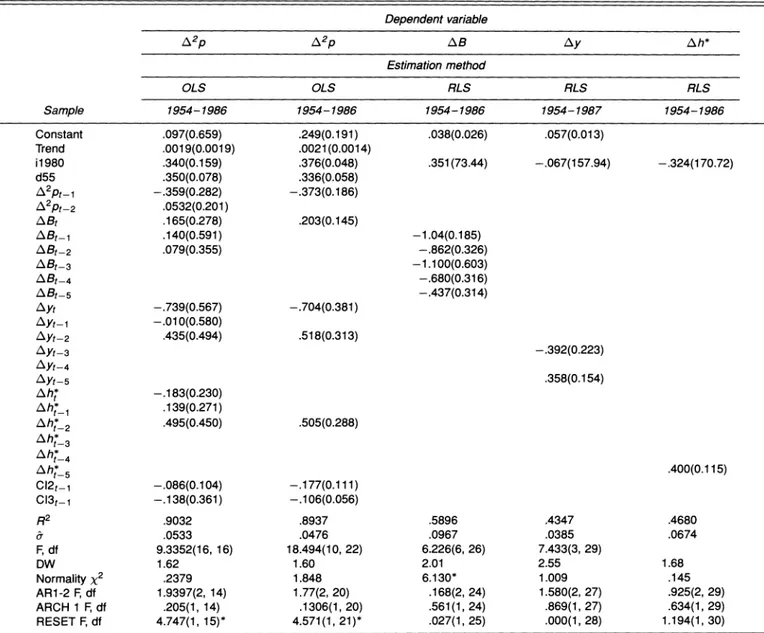
Metin: The Relationship Between Inflation and the Budget Deficit in Turkey 417 Table 4. The Conditional and Marginal Models
Dependent variable
A2p A2p AB Ay Ah*
Estimation method OLS OLS RLS RLS RLS Sample 1954-1986 1954-1986 1954-1986 1954-1987 1954-1986 Constant .097(0.659) .249(0.191) .038(0.026) .057(0.013) Trend .0019(0.0019) .0021(0.0014) il 1980 .340(0.159) .376(0.048) .351(73.44) -.067(157.94) -.324(170.72) d55 .350(0.078) .336(0.058) A2Pt-1 -.359(0.282) -.373(0.186) A2Pt-2 .0532(0.201) ABt .165(0.278) .203(0.145) ABt-1 .140(0.591) -1.04(0.185) ABt-2 .079(0.355) -.862(0.326) ABt-3 -1.100(0.603) A Bt4 -.680(0.316) ABt-5 -.437(0.314) Ayt -.739(0.567) -.704(0.381) Ayt-1 -.010(0.580) AYt-2 .435(0.494) .518(0.313) Ayt-3 -.392(0.223) AYt-4 Ayt-5 .358(0.154) Ahb* -.183(0.230) Aht,_ .139(0.271) Ah_2 .495(0.450) .505(0.288)
Ah_
t-3Ah_
t-4 Ah*_5 .400(0.115) CI2t-1 -.086(0.104) -.177(0.111) CI3t- -.138(0.361) -.106(0.056) R2 .9032 .8937 .5896 .4347 .4680 & .0533 .0476 .0967 .0385 .0674 F, df 9.3352(16, 16) 18.494(10, 22) 6.226(6, 26) 7.433(3, 29) DW 1.62 1.60 2.01 2.55 1.68 Normality X2 .2379 1.848 6.130* 1.009 .145 AR1-2 F, df 1.9397(2, 14) 1.77(2, 20) .168(2, 24) 1.580(2, 27) .925(2, 29) ARCH 1 F, df .205(1, 14) .1306(1, 20) .561(1, 24) .869(1, 27) .634(1, 29) RESET F, df 4.747(1, 15)* 4.571(1, 21)* .027(1, 25) .000(1, 28) 1.194(1, 30)NOTE: The diagnostic checks for residual autocorrelation (AR 1-2F test with the degrees of freedom shown) confirm the choice of relevant lag, residual heteroscedaticity of the ARCH form (ARCH 1 F test) suggested by Engle (1982). RESET-F is a regression specification test. It tests the null of correct specification of the original model against the alternative that powers of the dependent variable are present.
White (1980) estimated standard errors are in parenthe- ses. A2p depends on its own first lag and the current scaled public-sector deficit. It is also influenced by real income growth, its second lag, and the lagged monetization of the economy. The time trend and dummies have an impact on inflation. Equation (8) suggests a positive relationship between inflation and an appropriately scaled deficit. The ECM's explain the behavior of inflation by revealing rela- tively rapid reactions. This model closely matches the the- ory model and appears statistically satisfactory from the diagnostic tests except for the RESET F.
Parameter constancy is also an important statistical prop- erty. To examine constancy, recursive least squares is used because sequences of constancy tests yield tools for in- vestigating constancy from the corresponding one-step in- novations. From the sequence of innovations, Chow tests can be constructed for parameter constancy [distributed as F(1, t - k - 1) on the null]. Graphs provide a convenient way of portraying evidence about constancy. Figure 5 shows
the recursively estimated coefficients of variables in (8) and plus or minus twice their recursively estimated standard er- rors. Coefficients vary only slightly relative to their ex ante standard errors. Figure 5 also records one-step residuals and corresponding calculated equation standard errors for conditional inflation equation with 0 ? 2 estimated standard errors. The equation standard error varies little. Figure 5 finally plots the breakpoint Chow (1960) statistic for the inflation equation, which remains constant over the sample period considered.
4.2 Nonconstancy of Marginal Models
Nonconstancy of the marginal models is related to the concept of super exogeneity, which implies that the param- eters of the conditional model remain constant, even while those of the marginal model change (i.e., the Lucas critique does not hold). This subsection estimates marginal models for Ay, AB, and Ah*. Because of the results in Section 3.2, the parameters of interest here include just the parameters
418 Journal of Business & Economic Statistics, October 1998
Constant = Trend = A2LP.1=
+ 2S.E.= ... + 2S.E. = ... 2SE =.
.9 - . 8 - .6 "99 .4 . ..3. - , . ... ... . , 9.004- .3
4.3
.
S... ,':. ... ... ..' . .. . ... -. e99- -.6 -.3 .-.912 -9 1975 1980 1985 1990 1975 1980 1985 1998 1975 1980 1985 1990ABt = Ayt = Ayt-2 =.
+ 2S.E. =.. + 2SE. =... + 2SE.=
8 1 .6 - , .4 .8 .4 - .69 . - .2 - --.4 -.2-.8 ..2 .6 ... ? .. ... . -1.2 . Ah 2 012 = - Cl3' = - 6 .3 - 9 ... ... .'9 . .3 - -.1 / -.2... -.4 -.3 -.3- -.6 -.6 -.4 1975 1980 1985 1990 1975 1980 1985 1990 1975 1980 1985 1990 (a) .1 h - - Resi2StepW - CHOW
+22SE = .E.=..2 .. .. 1%crit= ...
-.1 -." ".. ---
Metin: The Relationship Between Inflation and the Budget Deficit in Turkey 419
ReslStep= N4 CHOWs=_ 1%. crit=...
S2 S. E ... 1.5- 18 1.2 ?0 .9 . .. .. .. . 1.2 . .. - ... t... .. . . ..6.- .09 ... -.18 -.27 0 1975 1980 1985 1990 1975 1980 .985 1990 (a) (b)
ReslStep= N4 CHOWs= I_.% cr it=
+ 2-S. E.=. .12- 1 - .08 - ... ... ... . ..8 .04 .6 1 /4 / .4 ..1 ... 1975 1980 1985 1990 1975 1980 1985 1990 (C) (d)
ReslStep=_ N4 CHOWs= IV. cit= ...
+ 2*S. E.-= .18 1- - 0..86 -.06 . ..4 -.18 .2 ... .... 1975 1980 1985 1990 1975 1980 t985 1990 (e) (f)
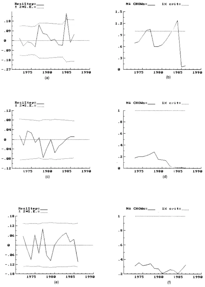
Figure 6. (a) One-Step Residuals From a Marginal Model for AB With 0 ? 2 Estimated Standard Errors; (b) Breakpoint Chow Statistics for a Marginal Model of AB Normalized by Their One-off 1% Critical Values; (c) One-Step Residuals From a Marginal Model for Ay With 0 f 2 Estimated Standard Errors; (d) Breakpoint Chow Statistics for a Marginal Model of Ay, Normalized by Their One-off 1% Critical Values; (e) One-Step Residuals From a Marginal Model for Ah* With 0 f 2 Estimated Standard Errors; (f) Breakpoint Chow Statistics for a Marginal Model of Ah*, Normalized by Their One-off 1% Critical Values.
for dynamics in the conditional model. For each marginal variable, we began with fifth-order autoregression (includ- ing a constant, trend, and i1980) and applied a sequential
reduction procedure. The results are reported in Table 4, columns 4-6. For AB all lags matter. The residuals are nonnormal. Figure 6, (a) and (b), graphs the one-step resid-
420 Journal of Business & Economic Statistics, October 1998 Table 5. Encompassing Test Statistics for Equation (8)
and Metin's (1995) Equation (9) Null hypothesis
Equation (8) Metin (1995) Statistic Distribution Distribution Cox N(0, 1) -2.75 N(0, 1) -7.39 Ericsson N(0, 1) 1.86 N(0, 1) 3.95 Sargan X2(6) 6.79 X2(9) 14.71 F F(6, 15) 1.19 F(9, 15) 2.63 & .0487% .0601% NOTE: T = 1954-1986.
uals and the sequence of breakpoint Chow statistics, which show considerable nonconstancy, with possible breaks in 1977 and 1984.
For Ay, the third and fifth lags matter. Statistically, the model appears well specified with no rejections from the diagnostic tests available. Figure 6, (c) and (d), plots the re- cursively estimated equation standard errors and the break- point Chow statistics. The marginal model of Ay appears constant.
For Ah*, only the fifth lag matters. The equation is sta- tistically satisfactory, and it appears constant [Fig. 6, (e) and (f)]. Because the conditional model for A2p is constant and the marginal model of AB is nonconstant, AB (at least) appears super exogenous for the dynamic parameters in the inflation equation.
4.3 Encompassing Implications of the Conditional Model A congruent model should encompass previous empir- ical findings explaining the same dependent variable (see Hendry and Richard 1982, 1989; Mizon and Richard 1986). Consider two rival explanations, denoted Ml and M2. The question was whether M2 can explain features of the data that Ml cannot. This can be a test of Ml, with M2 provid- ing an alternative to see whether M2 captures any specific information not embodied in Ml (see Doornik and Hendry 1994, p. 237). Several variants of encompassing have been proposed-variance (Cox 1961), parameter (Hendry 1983), reduced-form (Ericsson 1983), exogeneity (Hendry 1988), and forecast (Chong and Hendry 1986). In this subsection we compare Equation (8) with an inflation equation esti- mated by Metin (1995), using such encompassing tests. The model from Metin (1995) is
Apt = - .064 + 1.111Bt - 3.901A((G- T)/Y)t [.039] [.135] [.670] + 1.663Apv, + .229AECM-Mt [.362] [.099] - .272(ECM-UIP)t/2 + .074ECM-PPPt_1 [.093] [.044] + .257d55t - .234Ayt, (9) [.020] [.166]
where R2 = .8973,& = .0601, DW = 2.072, AR(2,26) = .55, ARCH: F(1,26) = 2.77, normality: X2(2) = 1.33, and RESET: F(1, 27) = 3.74. In the work of Metin (1995), ECM represents sectoral excess demands, where ECM-M,
ECM-PPP, and ECM-UIP were derived from the monetary sector, from purchasing power parity, and from uncovered interest-rate parity, and d55 is a dummy variable, which picks up a major outlier in 1955. Finally Ap, is consumer price index (CPI) inflation for industrial countries. Table 5 reports the encompassing test results. As shown in Table 5, Equation (8) variance dominates Equation (9) (.00487 vs. .0601). None of the encompassing tests reject (8), and all reject (9); the new model encompasses the old one. (Note that APtl was added to (8) to calculate the encompassing tests.)
5. CONCLUDING REMARKS
This article examines the relationship between the public- sector deficit and inflation. System cointegration analysis suggests three stationary relationships. Although weak ex- ogeneity does not hold for variables concerned (except Ay), one is still able to develop a conditional model for inflation. In that model, an increase in the scaled budget deficit imme- diately increases inflation. Real income growth has a nega- tive immediate effect and positive second-lag effect on in- flation. Monetization of the deficit also affects inflation at a second lag. These dynamics are consistent with institutional and general knowledge of the economy. The conditional model of inflation is constant over the sample period, even though several significant structural breaks occurred dur- ing the period. Breaks included three devaluations, struc- tural stabilization, and economic liberalization programs. As further evidence of its specification, the new conditional model of inflation encompasses the inflation equation of Metin (1995). The major finding from the new equation is that budget deficits (as well as real income growth and debt monetization) significantly affect inflation in Turkey.
ACKNOWLEDGMENTS
I am indebted to Neil Ericsson, David Hendry, and the referees for helpful comments. Ebru Voyvoda has provided valuable research assistance.
APPENDIX: DATA
This appendix describes the data, lists the definitions used, and gives their units and sources. The sample period is 1950-1987.
G, T: The budget expenditure (G) and the revenue (T) are the general budget expenditures and revenues from the bud- get and final accounts, respectively (TL Billion). Ministry of Finance and Custom General Directorate of Account- ing, Statistical Year Book of Turkey 1990, State Institute of Statistics Prime Ministry Republic of Turkey, Table No. 367, page 471.
G - T: The general budget deficit is the general budget ex- penditure minus the general budget revenue-that is, the primary deficit, which excludes interest payments (TL Bil- lion). The budget deficit does not include the SEE's deficit. Because reliable statistics about SEE's deficits are available only after the second half of the 1970s, the general budget deficit is therefore used as a proxy for the total deficit.
Metin: The Relationship Between Inflation and the Budget Deficit in Turkey 421
P: Price level is the CPI. The base year is 1980 (IMF In- ternational Financial Statistics, several issues).
Y: Y is nominal GNP, divided by the GNP deflator (TL Billion). Nominal GNP is obtained from IMF International Financial Statistics, several issues.
H: H is base money. The components of base money are currency in circulation, vault cash, legal reserves, and Cen- tral Bank sight deposits (TL Billion). Reserve money is ob- tained from the database of the Central Bank of Turkey.
[Received June 1995. Revised April 1998.]
REFERENCES
Ahking, F. W., and Miller, S. M. (1985), "The Relationship Between Gov- ernment Deficits, Money Growth and Inflation," Journal of Macroeco- nomics, 7, 447-467.
Aktan, R. (1964), "Analysis and Assessment of the Economic Effects, Pub- lic Law 480," The First Programme of Turkey, The State Planning Or- ganization Publication, Ankara.
Anand, R., and van Wijnbergen, S. (1989), "Inflation and the Financing of Government Expenditure: An Introductory Analysis With an Applica- tion to Turkey," The World Bank Economic Review, 3, 17-38.
Bhalla, S. S. (1981), "The Transmission of Inflation Into Developing Economies," in World Inflation and the Developing Countries, eds. W. R. Cline and Associates, Washington, DC: Brookings Institution, pp. 52-101.
Buiter, W. H., and Patel, U. R. (1992), "Debt, Deficits, and Inflation: An Application to the Public Finances of India," Journal of Public Eco- nomics, 47, 171-205.
Burdekin, R. C. K., and Wohar, E. M. (1990), "Deficit Monetisation, Output and Inflation in the United States, 1923-1982," Journal of Economic Studies, 17, 50-63.
Chong, Y. Y., and Hendry, D. F. (1986), "Econometric Evaluation of Linear Macro-Economic Models," Review of Economic Studies, 53, 671-690. Choudhary, M. A. S., and Parai, A. K. (1991), "Budget Deficit and Inflation:
The Peruvian Experience," Applied Economics, 23, 1117-1121. Chow, G. C. (1960), "Tests of Equality Between Sets of Coefficients in
Two Linear Regressions," Econometrica, 28, 591-605.
Cox, D. R. (1961), "Tests of Separate Families of Hypotheses," in Proceed- ings of the Fourth Berkeley Symposium on Mathematical Statistics and Probability (Vol. 1), ed. J. Neyman, Berkeley: University of California Press, pp. 105-123.
Dickey, D. A., and Fuller, W. A. (1981), "Likelihood Ratio Statistics for Autoregressive Time Series With a Unit Root," Econometrica, 49, 1057- 1072.
Dogas, D. (1992), "Market Power in a Non-monetarist Inflation Model for Greece," Applied Economics, 24, 367-378.
Doornik, J. A., and Hendry, D. F. (1994), PcGive Professional 8.0: An Inter- active Econometric Modelling System, London, International Thompson Publishing.
Dornbusch, R., and Fisher, S. (1981), "Budget Deficits and Inflation," in Development in an Inflationary World, eds. M. J. Flanders and A. Razin, New York: Academic Press.
Dwyer, G. P. (1982), "Inflation and Government Deficits," Economic In- quiry, 20, 315-329.
Engle, R. F. (1982), "Autoregressive Conditional Heteroscedasticity With Estimates of the Variance of United Kingdom Inflations," Econometrica, 50, 987-1007.
Engle, R. F., Hendry, D. F., and Richard, J.-F. (1983), "Exogeneity," Econo- metrica, 51, 277-304.
Ericsson, N. R. (1983), "Asymptotic Properties of Instrumental Variables Statistics for Testing Non-nested Hypotheses," Review of Economic Studies, 50, 287-304.
Fry, M. J. (1972), Finance and Development Planning in Turkey, Leiden: E. J. Brill.
- (1980), "Money, Interest, Inflation and Growth in Turkey," Journal of Monetary Economics, 6, 535-545.
Hamburger, M. J., and Zwick, B. (1981), "Deficits, Money and Inflation,"
Journal of Monetary Economics, 7, 141-150.
Hein, S. E. (1983), "Discussion," in The Economic Consequences of Gov- ernment Deficits, ed. L. H. Mayer, Boston: Kluwer Nijhoff, pp. 75-85. Hendry, D. F. (1983), "Comment," Econometric Reviews, 2, 111-114.
- (1988), "The Encompassing Implications of Feedback Versus Feed- forward Mechanism in Econometrics," Oxford Economic Papers, 40,
132-149.
Hendry, D. F., and Richard, J.-F. (1982), "On the Formulation of Empirical Models in Dynamic Econometrics," Journal of Econometrics, 20, 3-33. - 0(1989), "Recent Developments in the Theory of Encompassing,"
in Contributions to Operations Research and Economics: The Twentieth Anniversary of CORE, eds. B. Cornet and H. Tulkens, Cambridge, MA: MIT Press, pp. 393-440.
Ho, L. S. (1990), "Government Deficit Financing and Stabilisation," Jour- nal of Economic Studies, 17, 34-44.
Hondroyiannis, G., and Papapetrou, E. (1994), "Cointegration, Causality and Government Budget-Inflation Relationship in Greece," Applied Eco- nomic Letters, 1, 204-206.
Jarque, C. M., and Bera, A. K. (1980), "Efficient Tests for Normality, Homoscedasticity and Serial Independence of Regression Residuals," Economic Letters, 6, 255-259.
Johansen, S. (1988), "Statistical Analysis of Cointegration Vectors," Jour- nal of Economic Dynamics and Control, 12, 231-254.
- (1991), "Estimation and Hypothesis Testing of Cointegration Vec- tors in Gaussian Vector Autoregressive Models," Econometrica, 59,
1551-1580.
-0(1992a), "Cointegration in Partial Systems and the Efficiency of Single Equation Analysis," Journal of Econometrics, 52, 389-402. - (1992b), "Testing Weak Exogeneity and the Order of Cointegration
in UK Money Demand Data," Journal of Policy Modelling, 14, 313-334. Johansen, S., and Juselius, K. (1990), "Maximum Likelihood Estimation
and Inference on Cointegration-With Applications to the Demand for Money," Oxford Bulletin of Economics and Statistics, 52, 169-210. Juselius, K. (1992), "Domestic and Foreign Effects on Prices in an Open
Economy: The Case of Denmark," Journal of Policy Modelling, 14, 401- 428.
King, R. G., and Plosser, C. I. (1985), "Money Deficits and Inflation," in Understanding Monetary Regimes (Carnegie-Rochester Conference Series on Public Policy, 22), pp. 147-196.
Krueger, A. 0. (1974), Foreign Trade Regimes and Economic Development: Turkey, New York: National Bureau of Economic Research.
- (1995), "Partial Adjustment and Growth in the 1980s in Turkey," in Reform, Recovery, and Growth, eds. R. Dornbush and S. Edward, Chicago: University of Chicago Press, pp. 33-368.
Langdana, F. K. (1990), Sustaining Budget Deficits in Open Economies, London.
MacKinnon, J. G. (1991), "Critical Values for Cointegration Tests," in Long-run Economic Relationship: Readings in Cointegration, eds. R. F. Engle and C. W. J. Granger, Oxford, U.K.: Oxford University Press, pp. 267-276.
Metin, K. (1995), "An Integrated Analysis of Turkish Inflation," Oxford Bulletin of Economics and Statistics, 57, 513-533.
Mizon, G. E., and Richard, J.-F. (1986), "The Encompassing Principle and its Application to Testing Non-nested Hypotheses," Econometrica, 54, 657-678.
Okyar, O. (1965), "The Concept of Etatism," Economic Journal, 75, 99- 111.
Onis, Z., and Riedel, J. (1993), Economic Crisis and Long-Term Growth in Turkey (The Comparative Macro Economic Series), Washington, DC: The World Bank.
Osterwald-Lenum, M. (1992), "A Note With Quantiles of the Asymp- totic Distribution of the Maximum Likelihood Cointegration Rank Test Statistics," Oxford Bulletin of Economics and Statistics, 54, 461-472. Phelps, E. (1973), "Inflation and the Theory of Public Finance," Swedish
Journal of Economics, 75, 67-87.
Protopapadakis, A. A., and Siegel, J. J. (1987), "Are Money Growth and Inflation Related to Government Deficits? Evidence From Ten Industri- alized Economies," International Economic Journal, 3, 79-96.
Reimers, H.-E. (1992), "Comparisons of Tests for Multivariate Cointegra- tion," Statistical Papers, 33, 335-359.
422 Journal of Business & Economic Statistics, October 1998
Rodrik, D. (1990), "Premature Liberalization, Incomplete Stabilization: The Ozal Decade in Turkey," in Lessons of Economic Stabilization and its Aftermath, eds. M. Bruno, F. Stanley, E. Helpman, and N. Livitian, Cambridge, MA: MIT Press, pp. 323-353.
Sargent, T., and Wallace, N. (1981), "Some Unpleasant Monetarist Arithmetic," Quarterly Review, Federal Reserve Bank of Minneapolis, 5, 1-18.
Scarth, W. M. (1987), "Can Economic Growth Make Monetarist Arith-
metic Pleasant?" Southern Economic Journal, 53, 1028-1036.
Siddiqui, A. (1989), "The Causal Relation Between Money and Inflation in a Developing Economy," International Economic Journal, 3, 79-96. Sowa, N. K. (1994), "Fiscal Deficits, Output Growth and Inflation Targets
in Ghana," World Development, 22, 1105-1117.
White, H. (1980), "A Heteroskedasticity-consistent Covariance Matrix Es- timator and a Direct Test for Heteroskedasticity," Econometrica, 48, 817-838.