Growth optimal investment with threshold rebalancing portfolios under transaction costs

GROWTH OPTIMAL INVESTMENT WITH THRESHOLD REBALANCING PORTFOLIOS UNDER TRANSACTION COSTS

Sait Tunel, Mehmet A. Donmez2 and Suleyman S. Kozaf3

lGeorgia Institute of Technology, Industrial Engineering Department, Atlanta, USA 2Koc University, Electrical and Electronics Engineering Department, Istanbul, Turkey 3Bilkent University, Electrical and Electronics Engineering Department, Ankara, Turkey

ABSTRACT

We study how to invest optimally in a stock market having a finite number of assets from a signal processing perspective. In particular, we introduce a portfolio selection algorithm that maximizes the expected cumulative wealth in i.i.d. two­ asset discrete-time markets where the market levies propor­ tional trans action costs in buying and selling stocks. This is achieved by using "threshold rebalanced portfolios ", where trading occurs only if the portfolio breaches certain thresh­ olds. Under the assumption that the relative price sequences have log-normal distribution from the Black-Scholes model, we evaluate the expected wealth under proportional trans­ action costs and find the threshold rebalanced portfolio that achieves the maximal expected cumulative wealth over any investment period.

Index Terms- Portfolio management, threshold rebal­ ancing, transaction cost, discrete-time market, continuous dis­ tribution.

1. INTRODUCTION

Recently financial applications attracted a significant interest from the signal processing community since the recent global crises demonstrated the importance of sound financial mod­ eling and reliable data processing [1, 2]. Stock markets pro­ duce vast amount of temporal data ranging from stock prices to interest rates making them ideal mediums to apply signal processing methods. Furthermore, due to the integration of high performance, low-Iatency computing recourses and fi­ nancial data collection infrastructures, a wide range of signal processing algorithms could be readily leveraged with full po­ tential in stock markets. This paper specifically focuses on the portfolio selection problem, wh ich is one the most important financial applications and has already attracted substantial in­ terest from the signal processing cOlmnunity [3-8].

Determination of the optimum portfolio and the best port­ folio rebalancing strategy that maximize wealth in discrete­ time markets with no transaction lees is heavily investigated

in information theory [9, 10], machine learning [11-l3] and

signal processing [14-17] fields. Assuming that the portfolio rebalancings, i.e., adjustments to the portfolio by buying and selling stocks, require no transaction fees and with some fur­ ther mild assumptions on the stock prices, the portfolio that achieves the maximum expected wealth is shown to be a con­ stant rebalanced portfolio (CRP) [10, 18]. A CRP is a portfo­ lio strategy where the distribution of funds over the stocks are

reallocated to a predetermined structure, also known as the target portfolio, at the start of each investment period. How­ ever, we emphasize that maintaining a CRP requires poten­ tially significant trading due to possible rebalancings at each investment period [14]. As shown in [14], even the perfor­ mance of the best CRP is severely affected by moderate trans­ action fees rendering CRPs ineffective in real life stock mar­ kets. Clearly, one can potentially obtain significant gain in wealth by incIuding unavoidable transactions fees in the mar­ ket model and perform reallocation accordingly.

In these Iines, the optimal portfolio selection prob­ lem under transactions costs is extensively investigated for continuous-time markets [19-22], where growth optimal poli­ cies that keep the portfolio in cIosed compact sets by trading only when the portfolio hits the compact set-boundaries are introduced. It has been shown in [23] that under certain mild assumptions on the sequence of stock prices, similar no trade zone portfolios achieve the optimal growth rate even for discrete-time markets under proportional transaction costs. For markets having two stocks, i.e., two-asset stock markets, these no trade zone portfolios correspond to threshold port­ folios, i.e., the no trade zone is defined by thresholds around the target portfolio. In particular, unlike a calendar rebalanc­ ing portfolio, e.g., a CRP, a threshold rebalanced portfolio (TRP) rebalances by buying and selling stocks only when the portfolio breaches the preset boundaries, or "thresholds ", and otherwise does not perform any rebalancing. Intuitively, by limiting the number of rebalancings due to these non rebal­ ancing regions, threshold portfolios are able to avoid hefty transactions costs associated with excessive trading unlike calendar portfolios. Although TRPs are shown to be opti­ mal in i.i.d. discrete-time two-asset markets (under certain technical conditions) [23], finding the TRP that maximizes the expected growth of wealth under proportional transaction costs is not solved, except for basic scenarios [23], to the best of our knowledge.

In this paper, we first evaluate the expected wealth achieved by a TRP over any finite investment period given any target portfolio and threshold for two-asset discrete-time stock markets subject to proportional transaction fees. We emphasize that we study the two-asset market for notation al simplicity and our derivations can be readily extended to markets having more than two assets as provided in the paper where needed. We consider i.i.d. discrete-time markets repre­ sented by the sequence of price relatives (defined as the ratio of the cIosing prices of stocks in consecutive days), where

the sequence of price relatives follow log-normal distribu­ tions. Note that the log-normal distribution is the assumed statistical model for price relative vectors in the well-known Black-Scholes model [24, 25] and this distribution is shown to accurately model real life stock prices by many empirical studies [24]. Under this setup, we provide an iterative relation that efficiently and recursively calculates the expected growth over any period in any i.i.d. discrete-time market. This ex­

pected growth is then optimized by a brute force method to yield the optimal target portfolio and threshold to maximize the expected wealth over any investment period. We also illustrate the performance of our algorithm under different scenarios demonstrating its effectiveness.

We begin with the detailed description of the market and the TRPs in Section 2. We then calculate the expected wealth using a TRP in an i.i.d. two-asset discrete-time market un­ der proportional transaction costs over any investment period in Section 3. We provide an iterative relation to recursively calculate the expected wealth growth. The paper is then con­ cluded with the simulations of given algorithm in Section 4.

2. PROBLEM DESCRIPTION

In this paper, all vectors are column vectors and represented by lower-case bold letters. Consider a market with m stocks and let { x( t)

h>

1 represent the seq uence of price relative vec­ tors in this market, where x(t) = [X1(t),X2(t), ... , Xm(t)]T with Xi(t) E lR+ for i E {l, 2, ... , m} such that Xi(t) rep­ resents the ratio of the closing price of the ith stock for the tth trading period to that from the (t - 1 )th trading period. At each investment period, say period t, b ( t) represents the vector of portfolios such that bi (t) is the fraction of money in­ vested on the ith stock. We allow only long-trading such that

2::;:1 bi (t) = 1 and

b

i (t) ;::: O. After the price relative vector x(t) is revealed, we earn bT(t)x(t) at the period t.

We denote a TRP with a target vector b and a threshold

_E

(with certain abuse of notation) as "TRP with (b ,

E)".

For a sequence of price relatives vectors xn

�

[x(1), x(2), ... , x( n )] with x E lR;t;" a TRP with (b ,

E)

rebalances the portfolio to b at the first time T satisfying

bj

n;=l X

j

(t) ,-f

[ ]

,\,m

b

nr x (t) 'F-

bj -Ej, bj + Ej

�k=l k t=l k

(1)

for any j E {1, 2, ... , m}, thresholds

Ej,

and does not re­ balance otherwise, i.e., while the portfolio vector stays in the no rebalancing region. Starting from the first period of a no rebalancing region, i.e., where the portfolio is rebalanced to the target portfolio b, say t = 1 for this example, the wealth gained during any no rebalancing region is given by

m _n

S(xnlbn E

[�C)

=

L

b

k

rr

Xk(t), (2) k=l t=l

where bn = [b(1), b(2), ... , b(n)], b(t) is the portfolio at the period t and

[�C

is the length n no rebalancing region defined as

[�C

= {bn

I

b(1) = b ,

bj(t)

E

(bj -Ej, bj + Ej),

jE{1,2, ... ,m},tE{1,2, ... ,n}}. (3)

A TRP pays a transaction fee when the portfolio vector leaves the predefined no rebalancing region, i.e., goes out of the no rebalancing region

[�C,

and rebalanced back to its target port­ folio vector b. Since the TRP may avoid constant rebalanc­ ing, it may avoid excessive trans action fees while securing the portfolio to stay close to the target portfolio b, when we have heavy trans action costs in the market.

For notational clarity, in the remaining of the paper, we assume that the number of stocks in the market is equal to 2, i.e., m = 2. Note that our results can be readily extended to the case when m > 2. Then, the threshold rebalanced portfolios are described as folIows.

Given a TRP with target portfolio b = [b,1 - b]T with

b

E [0,1] and a threshold

E,

the no rebalancing region of a TRP with (b ,

E)

is represented by

(b -E, b + E).

Given a TRP with

_{(b - E, b + E),}

we only rebalance if the portfolio leaves this region, which can be found using only the first entry of the portfolio (since there are two stocks), i.e., if

_{b1,old (t) rf­}

(b -E, b + E).

In this case, we rebalance

b1,old (t)

to

b.

In this paper, we assume that the price relative vectors have a log-normal distribution following the well-known Black-Scholes model [24]. This distribution, wh ich is ex­ tensively used in the financial literature, is shown to model empirical price relative vectors close to accurate in many tests [26]. Hence, we assume that x(t) = [Xl (t), X2(t)]T has an i.i.d. log-normal distribution with mean

I.L

= [Ml, M2l and standard deviation a = [0'1,0'2], respectively, i.e., x(t) rv

InN(I.L,

a2).

3. THRESHOLD REBALANCED PORTFOLIOS

In this section, we analyze the TRPs in a discrete-time mar­ ket with proportional transaction costs as defined in Section 2. We first introduce an iterative relation, as a theorem, to recur­ sively evaluate the expected achieved wealth of a TRP over any investment period. The terms in this iterative equation are calculated using a certain form of multivariate Gaussian integrals. We then use the given iterative equation to find the optimal

_E

and

_b

that maximize the expected wealth over any investment period.

3. 1. An Iterative Relation to CaIculate the Expected Wealth

In this section, we introduce an iterative equation to evaluate the expected cumulative wealth of a TRP with

(b -E, b + E)

over any period n, i.e., E[S(n)]. For a TRP with

_{(b-E, b+E),}

any investment scenario can be decomposed as the union of consecutive no-crossing blocks such that each rebalancing in­ stant, to the initial b, signifies the end of a block. Hence, based on this observation, the expected gain of a TRP between consecutive crossings, i.e. the gain during the no-rebalancing regions, is directly proportional to the overall wealth growth. Therefore, in the next we first calculate the conditional ex­ pected gain of a TRP over no rebalancing regions and then introduce the iterative relation based on these derivations.

For a TRP with

_{(b - E, b + E),}

we call a no rebalancing region of length n as "period n with no-crossing " such that the TRP with the initial and target portfolio b = [b, 1 - b] stays in the

(b -E, b + E)

interval for n - 1 consecutive investment periods and crosses one of the thresholds at the nth period.

We next calculate the expected gain of a TRP over any no­ crossing period as follows.

The wealth growth of a TRP with (b- E, b+E) for a period T with no-crossing can be written as [27]

T T

(4)

t=l

t=l

!:::,. !:::,.

where

(1

= b - 2c(b - b2), (2 = 1 - b + 2c(b - b2) for b + E hitting and

_{(1 �}

b+2c(b- b2), (2

_�

1- b- 2c(b- b2) for b- E hitting and c represents the symmetrical commission cost, to rebalance two stocks, i.e.,

bl,old

(T + 1) to b, and

b2,old

(T +

1) = 1-

h,old

(T + 1) to 1- b. Thus, the conditional expected

gain of a TRP conditioned on that the portfolio stays in a no rebalancing region until the last period of the region can be found by calculating the expected value of (4).

In order to calculate the expected wealth E[S(n)] itera­ tively, let us first define the variable R(T), wh ich is the ex­ pected cumulative gain of all possible portfolios that hit any of the thresholds first time at the Tth period, i.e.,

(5) where

E�c

denotes the set of all possible portfolios with initial portfolio band that stay in the no rebalancing region for T -1 consecutive periods and hits one of the b - E or b + E boundary at the Tth period, i.e.,

E!C

_�

{bT E ßT(b, E)

I

b(l) = b, b(i) E (b - E, b + E) ViE{2, . . . , T- 1} , b(T)if-(b- E, b + E) }. (6) Here, ßT(b, E) is defined as the set of all possible threshold rebalanced portfolios with initial and target portfolio band a no rebalancing interval (b - E, b + E). Similarly we define the variable T( T), which is the expected growth of all possible portfolios of length T with no threshold crossings, i.e.,

(7)

where

E�c

denotes the set of portfolios with initial portfolio band that stay in the no rebalancing region for T consecutive periods, i.e., I

E�C

�

{bT E ßT(b, E)

I

b(l) = b, b(i) E [b - E, b + E] Vi E {2, . . . , Tn. (8) Given the variables R(T) and T(T), we next introduce a theorem that iteratively calculates the expected wealth growth of a TRP over any period n. Hence, to calculate the expected achieved wealth, it is sufficient to calculate R( T), T( T), threshold crossing probabilities P

(

bn E

E:n

and P (bn E

E�C),

which are explicitly evaluated in the next section.

'nlis is the special case of the definition in (3) for m = 2.

Theorem 3. 1 The expected wealth growth of a TRP (b-E, b+ E) , i.e., E[S(n)], over any i.i.d. sequence of price relative vectors xn = [x(l) , x(2) , . . . , x(n)], satisfies

n

E[S(n)] =

L

P(E;C)R(i)E[S(n -i)]

+

P(E�C)T(n), (9)

i=l

where we define So = 1, R(n) in (5) , T(n) in (7) ,

Efc

in (6) and

E�c

in (8).

The proof of the Theorem 3.1 can be found in [27]. Theo­

rem 3.1 provides a recursion to iteratively calculate the ex­

pected wealth growth E[S(n)], when R(T) and T(T) are ex­ plicitly calculated for a TRP with (b - E, b + E). Hence, if we can obtain P

(E�c)

R( T) and P

(E�C)

T( T) for any T, then (9) yields a simple iteration that provides the expected wealth growth for any period n. We next give the explicit definitions of the events b T E

E�c

and b T E

E�c

in order to calculate the conditional expectations R( T) and T( T). Following these definitions, we calculate P

(E�c)

R(T) and P

(E�C)

T(T) to evaluate the expected wealth growth E[S( T)], iteratively from Theorem 3.1 and find the optimal TRP, i.e., optimal band E,

by using a brute force search.

We next provide the conditions for the market portfolios to cross the corresponding thresholds and calculate the prob­ abilities for the events bT E

E�c

and bT E

E�c.

We then calculate the conditional expectations R( n) and T( n) as cer­ tain multivariate Gaussian integrals.

Hence, we can explicitly describe the event that the mar­ ket threshold portfolio (b - E, b + E) does not hit any of the thresholds for T consecutive periods, b T E

E�c,

as the inter­ section of the events as [27]

bT E E�c ==

n

h2Ih(i) ::::; Ih(i) ::::; '")'1Ih(i)}, (10) i=l

where Ih(i)

_�

_n�=l

_X

_l

_{(t), Ih(i)}

_�

_n�=l

_X2(t) ,"1'1 !:::,.

b(1-b+E)

_{d !:::,.}

_b(1-b-E)

_{S' '1 1 h f h}

(l-b)(b-E)

an '"'(2 =

(l-b)(bH)'

11lll ar y, t e event 0 t e

market threshold portfolio (b - E, b + E) hitting any of the thresholds first time at the T-th period, bT E

E�c,

can be de­ fined as the intersections of the events [27]

T-1

bT E [�C ==

n

h2II1(i) ::::; II2(i) ::::; 11II1(i)} i=l

(11)

yielding the explicit definitions of the events b T E

E�c

in (11)

and bT E

E�c

in (10). The definitions of _bT E

E�c

and bT E

E�c

can be readily extended for the case m > 2 by using the updated definitions of IIl, II2, . . . , IIm.

Using the quantitative definitions of the events bT E

E�c

and bT E

E�c,

we can express P

(E�C)

T(T) as [27]

P (E�C) T(T) =

{OO

j"Y17l"1

(b1l"l

+ (1-

b)1l"2) P(II1(T) = 1l"1,

Jo

/'27rl

II2(T) = 1l"2)P

(

�; E [�-(h, � -82], �3 E [�-81, � -82],

wh ich follows from the definition of

��

_< where

r;,

�

In

71"2

71"1

• The first probability in (12) can be caIculated as [27]

wh ich follows since

II1(T)

_�

n;=1 Xl(t)

and

II2 (T)

_�

n;=IX2(t)

and we have

II1(T)

rv

InN (TJ-il,mi)

and

II2(T)

rv

InN(TJ-i2, Td).

Similarly we can express

P ([�C) R (T)

as [27] P

_([;c)

R(T) =

r= 1=

((17l"1 + (27l"2) P(Ih(T) = 7l"1,

Ja ')'17("1

Ih(T) =7l"2)P

₍

�; E [1\;-81,1\;-82],�� E [1\;-81,1\;-82]

r=

('I27r1

, ... ,�� E [I\;-81,1\;-82]

₎

d7l"2d7l"1+

Ja Ja

((37l"1 + (47l"2)

P(Ih(T) = 7l"1, Ih(T) = 7l"2)P

₍

�; E [I\; -81, K -82],

... ,�� E [1\;-81,1\;-82]

₎

d7l"2d7l"1 , (14)

where the probability

P(II1 (T)

=

7l"1,II2(T)

=

7l"2)

can be obtained via (l3).

Hence to caIculate

P ([�C)T(T)

and

P ([�C) R(T),

we need to caIculate the probability

_p(

�2

E

[r;, BI, r;,

-B2],�3

E

[r;,-Bl,r;,-B2], . . . ,��

E

[r;,-B1,r;,-B2l

₎

in (12)

and (14). We emphasize that the given multivariate probabil­ ity cannot be caIculated in a closed form [28], however there are some algorithms proposed in the literature to caIculate it with small errors. In this paper, we use the randomized Quasi-Monte Carlo (QMC) algorithm, provided in [27, 28].

4. SIMULATIONS

In this section, we illustrate the performance our algorithm under different scenarios. We use our algorithm over the his­ torical data set collected from the New York Stock Exchange over a 22-year period [9, 14] and illustrate the average perfor­ mance. In these simulations, we compare the performance of our algorithm with portfolio selection strategies from [9, 14, 29].

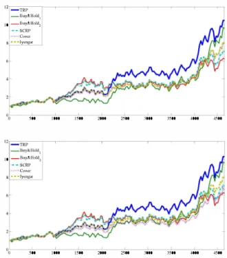
To remove any bias on a particular stock pair, we show the average performance of the TRP algorithm over randomIy selected stock pairs from the historical data set from [9]. The total set includes 34 different stocks, where the Iroquois stock is removed due to its peculiar behavior. We first randomly se­ lect pairs of stocks and invest using: the sequential TRP al­ gorithm with the sequential ML estimators, the Cover's uni­ versal portfolio algorithm, the Iyengar's universal portfolio algorithm and the SCRP algorithm. The sequential selection of the optimal TRP parameters are performed similar to the previous case, i.e., we use ML estimators on an investment block of 1000 days and use the caIculated optimal TRP in the next block of 1000 days. For each stock pair, we simulate the performance of the algorithms over 4651 days. In Fig. 1, we

12_TRP _Buy&Holdl IO-Buy&Hold1 '·'·'SCRP """'Cover s···lyengar 500 1000 1500 2000 2500 3000 3500 4000 4500 12'_---=TR�P -,--,---,---,----,----,---,--,----,-, _ßuy&Holdl 10 _ßuy&Hold1 '·'·'SCRP 1I"'''Cover S·· .. lycngar 500 1000 1500 2000 2500 3000 3500 4000 4500

Fig. 1. Average performance of various portfolio invest­

ment algorithms on independent stock pairs under a moderate (c=O.OI) and a hefty transaction cost (c=0.025).

present the wealth achieved by these algorithms, where the results are averaged over 10 independent trials. We present the achieved wealth over random sets of stock pairs under a hefty transaction cost c = 0.025 and a moderate transaction cost c = 0.01, where c is the fraction paid in commission for each transaction, i.e., c = 0.01 is a 1 % cOlmnission, in Fig. 1. We observe that the performance of the TRP algorithm read­ ily outperforms the other algorithms for different transaction costs on this historical data set. Moreover, the relative gain is larger for the large transaction cost since the TRP approach, with the optimal parameters chosen as in this paper, can hedge more effectively against the trans action costs.

5. CONCLUSION

In this paper, we studied an important financial application, the portfolio selection problem, from a signal processing per­ spective. We investigated the portfolio selection problem in i.i.d. discrete-time markets having a finite number of assets, when the market levies proportional transaction fees for both buying and selling stocks. We introduced algorithms based on threshold rebalanced portfolios that achieve the maximal growth rate when the sequence of price relatives have the log-normal distribution from the well-known Black-Scholes model [24]. Under this setup, we provide an iterative relation that efficiently and recursively caIculates the expected wealth in any i.i.d. market over any investment period. As predicted from our derivations, we significantly improve the achieved wealth over portfolio selection algorithms from the literature on the historical data set from [9].

6. REFERENCES

[1] IEEE Journal of Selected Topics in Signal Processing, "Special issue on signal processing methods in finance and electronic trading, " .

[2] IEEE Signal Processing Magazine, "Special issue on signal processing for financial applications, " .

[3] A. J. Bean and A. C. Singer, "Universal switching and side information portfolios under transaction costs us­ ing factor graphs," IEEE Journal of Selected Topics in Signal Processing, vol. 6, no. 4, pp. 351-365, August 2012.

[4] A. Bean and A. C. Singer, "Factor graphs for universal portfolios, " in Proceedings of the Forty-Third Asilomar Conference on Signals, Systems and Computers, 2009, pp. 1375-1379.

[5] M. U. Torun, A. N. Akansu, and M. AvelIaneda, "Port­ folio risk in multiple frequencies, " IEEE Signal Pro­ cessing Magazine, vol. 28, no. 5, pp. 61-71, Sep 2011.

[6] A. Bean and A. C. Singer, "Universal switching and side information portfolios under transaction costs using factor graphs, " in Proceedings ofthe ICASSP, 2010, pp.

1986-1989.

[7] A. Bean and A. C. Singer, "Portfolio selection via con­ strained stochastic gradients, " in Proceedings of the SSP, 2011, pp. 37-40.

[8] M. U. Torun and A. N. Akansu, "On basic price model and volatility in multiple frequencies, " in Proceedings ofthe SSP, June 2011, pp. 45-48.

[9] T. Cover, "Universal portfolios, " Mathematical Fi­ nance, vol. 1, pp. 1-29, January 1991.

[10] T. Cover and E. Ordentlich, "Universal portfolios with side-information, " IEEE Transactions on Information Theory, voI. 42, no. 2, pp. 348-363, 1996.

[11] D. P. Helmbold, R. E. Schapire, Y. Singer, and M. K.

Warmuth, "Online portfolio selection using multiplica­ tive updates, " Mathematical Finance, vol. 8, pp.

325-347, 1998.

[12] Y. Singer, "Swithcing portfolios, " in Proc. of Conj. on Uncertainty in AI, 1998, pp. 1498-1519.

[13] V. Vovk and C. Watkins, "Universal portfolio selection, " in Proceedings ofthe COLT, 1998, pp. 12-23.

[14] S. S. Kozat and A. C. Singer, "Universal semiconstant rebalanced portfolios, " Mathematical Finance, vol. 21,

no. 2, pp. 293-311, 2011.

[15] S. S. Kozat and A. C. Singer, "Switching strategies for sequential decision problems with multiplicative loss with application to portfolios, " IEEE Transactions on Signal Processing, vol. 57, no. 6, pp. 2192-2208, 2009.

[16] S. S. Kozat and A. C. Singer, "Universal switching port­ folios under trans action costs, " in Proceedings of the ICASSP, 2008, pp. 5404-5407.

[17] S. S. Kozat, A. C. Singer, and A. 1. Bean, "A tree­

weighting approach to sequential decision problems with multiplicative loss, " Signal Processing, vol. 92,

no. 4, pp. 890-905, 2011.

[18] T. M. Cover and C. A. Thomas, Elements of Information Theory, Wiley Series, 1991.

[19] M. H. A. Davis and A. R. Norman, "Portfolio selec­ tion with transaction costs, " Mathematics of Operations Research, vol. 15, pp. 676713, 1990.

[20] M. Taksar, M. Klass, and D. Assaf, "A diffusion model for optimal portfolio selection in the presence of broker­ age fees, " Mathematics ofOperations Research, vol. 13, pp. 277-294, 1988.

[21] A. J. Morton and S. R. Pliska, "Optimal portfolio man­ angement with transaction costs, " Mathematical Fi­ nance, vol. 5, pp. 337-356, 1995.

[22] M. J. P. Magill and G. M. Constantinides, "Portfolio

selection with transactions costs, " Journal of Economic Theory,vol. 13, no. 2, pp. 245-263, 1976.

[23] G. Iyengar, "Discrete time growth optimal investment with costs, " hup:/ /www.ieor.columbia.eduJ gi 1 O/Papers/stochastic. pdf. [24] D. Luenberger, Investment Science, Oxford University

Press, 1998.

[25] H. Markowitz, "Portfolio selection, " Journal of Fi­ nance,vol. 7, no. 1, pp. 77-91, 1952.

[26] Z. Bodie, A. Kane, and A. Marcus, Investments, McGraw-Hill/lrwin, 2004.

[27] S. Tunc and S. S. Kozat, "Optimal investment under transaction costs: A threshold rebalanced portfolio ap­ proach, " http://arxiv.org/pdf/1203.4156v1.pdf.

[28] A. Genz and F. Bretz, Computation of Multivariate Nor­ mal and t Probabilities, Springer, 2009.

[29] G. lyengar, "Universal investment in markets with trans­ action costs, " Mathematical Finance, vol. 15, no. 2, pp.