Bounding volume hierarchy-tetrahedralization hybrid acceleration structure for ray tracing

(1)

BOUNDING VOLUME

HIERARCHY-TETRAHEDRALIZATION

HYBRID ACCELERATION STRUCTURE

FOR RAY TRACING

a thesis submitted to

the graduate school of engineering and science

of bilkent university

in partial fulfillment of the requirements for

the degree of

master of science

in

computer engineering

By

Serkan Demirci

December 2020

(2)

Bounding Volume Hierarchy-Tetrahedralization Hybrid Acceleration Structure for Ray Tracing

By Serkan Demirci December 2020

We certify that we have read this thesis and that in our opinion it is fully adequate, in scope and in quality, as a thesis for the degree of Master of Science.

U˘gur G¨ud¨ukbay(Advisor)

¨

Ozcan ¨Ozt¨urk

Yusuf Sahillio˘glu

Approved for the Graduate School of Engineering and Science:

Ezhan Kara¸san

(3)

ABSTRACT

BOUNDING VOLUME

HIERARCHY-TETRAHEDRALIZATION HYBRID

ACCELERATION STRUCTURE FOR RAY TRACING

Serkan Demirci

M.S. in Computer Engineering Advisor: U˘gur G¨ud¨ukbay

December 2020

The computational cost of the ray-tracing method is directly proportional to the number of ray-surface intersection tests. The naive ray-tracing algorithm requires _{O(N) computational cost for the ray-surface intersection calculations} where N is the number of primitives in the scene. Ray tracing acceleration data structures like the regular grid, bounding volume hierarchy (BVH), kd-tree, constrained tetrahedralization, has been developed to reduce the number of ray-object intersection tests to speed-up ray tracing.

We propose a hybrid acceleration structure, the Bounding Volume Hierarchy-Tetrahedral mesh hybrid (BTH) acceleration structure, that can be used to speed-up ray tracing. BTH structure is composed of a BVH hierarchy where some of the leaves of the BVH hierarchy contain tetrahedralizations. We propose an algorithm for the construction of the BTH structure. We describe methods for approximating the average nearest-hit cost of a tetrahedralization, which we use for the construction of BTH. Besides, we can adapt the proposed BTH structure for dynamic scenes with hierarchical motion. We describe a two-level BVH-BTH acceleration structure for rendering animated scenes.

We test the proposed BTH structure using various scenes. For some of the experiments, the BTH structure performs better against other acceleration struc-tures in terms of rendering times. We perform experiments for animated scenes. We show that the two-level BTH structure outperforms the two-level BVH struc-ture for the tested dynamic scenes.

Keywords: Ray tracing, acceleration structure, tetrahedralization, Bounding Vol-ume Hierarchy, k-d tree.

(4)

¨

OZET

IS¸IN ˙IZLEME ˙IC

¸ ˙IN SINIRLAYICI HAC˙IM

H˙IYERARS¸˙IS˙I-D ¨

ORTY ¨

UZLEME H˙IBR˙IT

HIZLANDIRICI YAPISI

Serkan Demirci

Bilgisayar Mühendisli˘gi, Yüksek Lisans Tez Danı¸smanı: U˘gur Güdükbay

Aralık 2020

I¸sın izleme yönteminin hesaplama maliyeti ı¸sın-yüzey kesi¸sim testlerinin sayısı ile do˘gru orantılıdır. I¸sın izleme i¸cin ı¸sın-yüzey kesi¸sim testlerinin hesaplama za-manı naif algoritma i¸cin_{O(N) olup N sahnedeki nesne sayısıdır. Düzenli ızgara,} sınırlayıcı hacim hiyerar¸sisi (BVH), kd a˘gacı, kısıtlı dört yüzlüle¸stirme gibi ı¸sın izleme hızlandırma veri yapıları, ger¸cek zamanlı ı¸sın izleme elde etmek i¸cin ı¸sın-nesne kesi¸sim testlerinin sayısını azaltmak i¸cin geli¸stirilmi¸stir.

I¸sın izlemeyi hızlandırmak i¸cin kullanılabilecek bir hibrit hızlandırma yapısı, Sınırlayıcı Hacim Hiyerar¸sisi-D¨orty¨uzleme hibrit (BTH) hızlandırma yapısı ¨

oneriyoruz. BTH yapısı, BVH hiyerar¸sisinin bazı yapraklarının dörtyüzlü örgüler i¸cerdi˘gi bir BVH hiyerar¸sisinden olu¸sur. BTH yapısının olu¸sturulması i¸cin bir algoritma öneriyoruz. BTH yapısının olu¸sturulması i¸cin kullandı˘gımız, dörtyüzlüle¸stirmenin ortalama en yakın isabet maliyetini tahmin etmek i¸cin yöntemler sunuyoruz. Ayrıca, önerilen BTH yapısını hiyerar¸sik hareketli dinamik sahneler i¸cin uyarlıyoruz. Dinamik sahneleri olu¸sturmak i¸cin iki seviyeli bir BVH-BTH hızlandırma yapısı sunuyoruz.

¨

Onerilen BTH yapısını ¸ce¸sitli sahneler kullanarak test ediyoruz. Bazı durum-larda BTH yapısı, i¸sleme süreleri a¸cısından di˘ger hızlandırma yapılarına göre daha iyi performans göstermektedir. Hareketli sahneler i¸cin deneyler yapıyoruz. ˙Iki seviyeli BTH yapısının iki seviyeli BVH yapısından daha iyi performans göstermektedir.

Anahtar sözcükler : I¸sın izleme, hızlandırıcı yapısı, dörtyüzleme, Sınırlayıcı Hacim Hiyerar¸sisi, k-d a˘gacı.

(5)

Acknowledgement

I would like to thank my advisor Prof. Dr. U˘gur G¨ud¨ukbay for his invaluable guidance throughout my research.

I would like to thank Aytek Aman providing feedback throughout all phases of my work.

I would like to thank all my friends for being helpful and supportive during my thesis study. Finally, my greatest thanks to my family. I am forever grateful. This work is supported by the Scientific and Technological Research Council of Turkey (T ¨UB˙ITAK) under Grant No. 117E881.

(6)

List of Figures

2.1 A uniform grid structure . . . 5

2.2 A k -d tree structure . . . 6

2.3 A bounding volume hierarchy (BVH). . . 8

2.4 Nearest-hit query on tetrahedralization . . . 10

3.1 Bounding Volume Hierarchy-Tetrahedralization hybrid (BTH) ac-celeration structure. . . 13

3.2 Finding the initial tetrahedron in a bounded tetrahedralization. . 17

4.1 The average depth estimation using depth map. . . 21

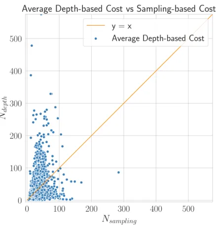
4.2 The comparison of the estimated tetrahedron count using the av-erage depth-based method and the sampling-based method. . . . 22

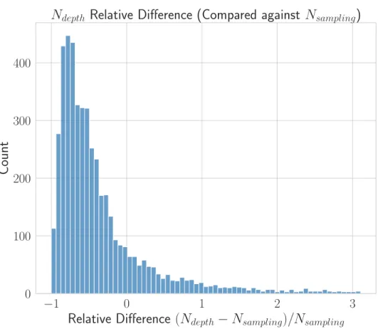
4.3 The histogram of the relative difference of the tetrahedron count between the average depth-based and sampling-based estimation methods. . . 23

4.4 The comparison of the estimated tetrahedron count using the av-erage depth-based method and the sampling-based method. . . 24

(9)

LIST OF FIGURES ix

4.5 The histogram of the relative difference of the tetrahedron count between the primitive count-based and the sampling-based estima-tion methods. . . 25

5.1 An instancing example. . . 28 5.2 Two-Level BVH-BTH structure. . . 29

6.1 Tetrahedralizations of the BTH structure constructed using differ-entCtet values. . . 32

6.2 Rotating armadillo animated scene rendered using the two-level BVH-BTH structure. . . 40 6.3 Random motion animated scene rendered using the two-level

BVH-BTH structure. . . 41 6.4 Falling airballs animated scene rendered using the two-level

(10)

List of Tables

6.1 BTH32 statistics for varyingCtet. . . 33

6.2 BTH20 statistics for varyingCtet. . . 34

6.3 The comparison of the construction and rendering times for dif-ferent acceleration structures on scenes that cannot be directly tetrahedralized. . . 37 6.4 The comparison of the construction and rendering times for

differ-ent acceleration structures on scenes that can be directly tetrahe-dralized. . . 38 6.5 The comparison of the construction and rendering times for

(11)

Chapter 1 Introduction

1.1 Motivation

Ray tracing [1] is a rendering method that generates photo-realistic images by simulating the interaction of lightpaths between objects. One of the most fun-damental operations used in ray tracing is ray-surface intersection tests. In ray tracing, a significant amount of computational time is dedicated to finding the nearest surface that a ray hits. With the introduction of path tracing [2] for global illumination, the importance of fast nearest hit tests increased. Path tracing is a form of ray tracing that uses Monte Carlo method to generate realistic images. Path tracing requires large number of lightpaths to be simulated. The quality of the generated image in path tracing directly depends on the number of simulated lightpaths.

Given a scene and a ray, a naive way to find the nearest-hit requires Θ(N ) time, where N is the number of primitive surfaces in the scene. Θ(N ) time is slow for most of the ray-tracing algorithms. To speed-up the ray-surface intersection tests, various spatial acceleration structures, such as regular grids, octrees, k-d trees, bounding volume hierarchies, are proposed in the literature. Such spatial acceleration structures reduce the number of ray-surface intersection tests by

(12)

eliminating some of the candidate primitives. In ray tracing, substantial gains can be achieved by using such acceleration structures.

One alternative spatial acceleration structure is tetrahedralizations. Lagae and Dutr´e [3] proposed the use of constrained tetrahedralizations as spatial ac-celeration structure. Although constrained tetrahedralizations are alternatives to well-known acceleration structures, the limitations of tetrahedralization algo-rithms make them limited in real-world applications.

We propose a BVH-Tetrahedral mesh hybrid acceleration structure (BTH) as a spatial acceleration structure. BTH structure combines the strength of two acceleration structures BVH and tetrahedralizations.

1.2 Contributions

The main contributions of the thesis are as follows.

• We propose a hybrid acceleration structure, BTH, which is composed of a BVH and tetrahedralizations.

• We propose a construction method for the new hybrid structure

• propose methods to find approximate nearest-hit cost for the tetrahedral-ization acceleration structure.

• We show that just like BVH structure, hybrid structure can be adapted to the dynamic scenes.

(13)

1.3 Organization of the Thesis

The organization of the thesis is as follows. Chapter 2 summarizes the existing acceleration structures, their strengths, and weaknesses. Chapter 3 introduces introduces construction and nearest-hit traversal algorithms of the BTH acceler-ation structure. Chapter 4 describes the nearest-hit cost approximacceler-ation methods for tetrahedralization acceleration structure, which is used by BTH construction algorithm. Chapter 5 shows how BTH structure can be modified to be used for dynamic scenes. Chapter 6 presents the experimental setup and results of the experiments.

(14)

Chapter 2 Background and Related Work

The visibility test is one of the most fundamental operations for ray tracing. The naive, brute-force, visibility test algorithm checks every primitive in the scene with the ray to find the nearest intersection. The time complexity of the naive visibility algorithm (Θ(N )) makes it impractical for complex scenes. Acceleration structures reduce the complexity of visibility tests by decreasing the number of ray-primitive tests required. In this section, we discuss grids, k -d trees, and BVHs that are widely used in modern ray tracers. We also discuss tetrahedralizations as another acceleration structure for ray-surface intersections. We discuss the strengths and weaknesses of different acceleration structures.

2.1 Grids

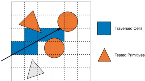
One of the basic nearest hit acceleration structure is uniform grids. Uniform grids [4] subdivide the scene space into uniform-sized cells (cf. Figure 2.1). Each cell stores a list of primitives that occupy the cell. Multiple cells can contain the same primitive if such primitive spans multiple cells. The nearest-hit traversal algorithm on grids, often referred to as the three-dimensional digital differential

(15)

Traversed Cells

Tested Primitives

Figure 2.1: A uniform grid structure

analyzer (3D-DDA) algorithm, visits each cell along the ray. In nearest-hit traver-sal, as each cell is traversed, all of the primitives in the cell’s list are checked for intersections. The traversal stops when a cell contains a primitive that intersects the ray. Since cells are checked in ray’s order, starting from the cell that ray’s origin resides in, along the ray’s direction.

The nearest-hit performance of uniform grids directly depends on the size of the cells. If cells are large, the grid will be less effective in reducing the number of ray-primitive intersection tests. On the other hand, if cells are small, more cells are needed to be traversed before finding the nearest-hit.

One other factor that affects the performance of uniform grids is the dis-tribution of primitives in the scene. Since uniform grids do not adapt to the distribution of primitives in the scene, the distribution of primitives in the scene directly affects the performance of the uniform grid. If primitives in the scene are distributed unevenly, occupancy of the cells will also be unevenly distributed. Empty cells and overpopulated cells will decrease the performance of the cells.

For the optimal grid sizes, different analyses are done in the literature ([5], [6], [7] and [8]). Clearly and Wyvill [5] showed that for scenes with N evenly distributed small, equally sized primitives, optimal case is to subdivide each axis

(16)

Tested Primitives

Figure 2.2: A k -d tree structure into √3 N cells, with minimum average Θ(√3

N ) time and O(N) space complexity.

2.2 K -d Trees

In k -d trees [9] scene is recursively divided into two half-spaces (cf. Figure 2.2). A primitive is associated with a half-space if the half-space contains a part of the primitive. If a primitive lies in both half-spaces it is included in both sub-trees.

The nearest-hit traversal in k -d trees starts from the root, in each split, half-spaces are tested for intersection in the ray’s traversal order. Traversal descends through the tree until a terminal node is reached. If a terminal node is encoun-tered, each primitive inside the terminal node is tested for intersection. Similar to grids, traversal stops when the first primitive intersection is found in a terminal node. The structure of the k -d trees and the axis and position of the splitting planes affect the nearest-hit test performance. In general, k -d trees are con-structed in a top-down manner using heuristics to find the best splitting plane. Given a split, heuristics estimate the cost of nearest-hit tests. Heuristics are also used as a terminating criterion for k -d tree construction.

(17)

Surface area heuristic (SAH) [10, 11] is the most commonly used heuristic for the construction of k -d trees. SAH estimates the expected cost of the nearest-hit test for a long uniformly distributed random ray. Given a split s, the SAH cost is calculated as

CostSAH(s) =

Ci

SA(s)(nlSA(l) + nrSA(r)) + Ct, (2.1) where the SA function calculates the surface area of the node’s bounding box. Ci constant is the cost of the ray-primitive intersection, Ct constant is the

cost of traversing a node. nl, and nr are the number of primitives in the left

and right half-spaces. The SAH-based k -d tree construction further improved by [12] and [13].

2.3 Bounding Volume Hierarchies

One of the popular spatial acceleration structures is bounding volume hierarchies (BHVs). BVHs are composed of a hierarchy of partitions where each partition is represented by a volume that encloses all of the primitives in that partition (cf. Figure 2.3). Unlike other acceleration structures, BVHs partition primitives instead of subdividing the scene space. Therefore, bounding volumes can inter-sect. Because BVHs partition primitives, primitives are not duplicated in BVHs, unlike k -d trees.

Bounding volumes in the hierarchy provide a simple method for finding the nearest-hit. If a ray does not pass through a bounding volume, primitives rep-resented by such bounding volume are not needed to be tested. Therefore, the nearest-hit algorithm (see Algorithm 1) recursively traverses the hierarchy in depth-first order. If the algorithm encounters an inner node, the algorithm checks whether a ray passes through the bounding volume. If the ray does not pass through the bounding volume, the algorithm does not traverse its children. If the algorithm encounters a leaf node, the algorithm checks each primitive with

(18)

Tested Primitives

Figure 2.3: A bounding volume hierarchy (BVH).

the ray for an intersection. Since BVHs bounding volumes can intersect, unlike space subdivision acceleration structures, the algorithm does not stop when the first intersection is found. The algorithm needs to test all possible nodes, before finding the nearest-hit.

Algorithm 1 Recursive BVH Nearest-hit traversal

1: _{procedure BVHIntersect(node, ray)} 2: if node is a leaf then

3: for all primitive in node do

4: _{Intersect(primitive, ray)} 5: else

6: for all children c of node do

7: _{BVHIntersect(c, ray)}

BVHs are first used by Clark [14] for visible surface determination. Later Rubin and Whitted [15] used them to accelerate ray tracing. In early BVH research, BVHs are constructed by hand. Kay and Kajiya [16] proposed an automatic top-down construction of BVHs using median splits. Goldsmith and Salmon [10] proposed SAH measure and used incremental insertions for construc-tion. Incremental construction with SAH measure leads to poor quality BVHs. M¨uller and Fellner [17] used SAH to build a BVH in a top-down manner. Later Wald et al. [18] used centroid-based SAH partitioning to improve top-down con-struction with Θ(N log2_{(N )) average construction complexity. Later streamed}

(19)

binning idea from k -d trees [19] are applied to BVHs by Wald [20] to further improve the runtime of the construction algorithm.

In general, modern BVH structures use Axis Aligned Bounding Boxes (AABB) as bounding volumes. The BVH tree is constructed from top to bottom using Surface Area Heuristics (SAH) to find the good primitive partitions.

2.4 Tetrahedralizations

Lagae and Dutr´e [3] first proposed constrained tetrahedralizations to accelerate nearest-hit tests for ray tracing. In two dimensions, the various forms of triangu-lation algorithms are defined as follows.

• Triangulation of a set of points S in a plane is a partition of the region of the convex hull of S into non-overlapping triangles, such that vertices of triangles are a superset of S.

• Delaunay triangulation of set of points S is a triangulation of S such that every triangle is Delaunay [21].

• Constrained Triangulation of points S, segments P is a triangulation that conforms points and segment constraints. A triangulation conforms to a constraint if it contains that constraint as a part of a triangle.

• Constrained Delaunay Triangulation of S points and constraints is a trian-gulation that whose triangles are constrained Delaunay and it conforms to given constraints.

Tetrahedralizations are three-dimensional equivalents of triangulations in a plane. Similarly, constrained tetrahedralization of a set of points, segments, and faces is a tetrahedralization that conforms to given constraints; points, segments, and faces. Many tetrahedralization algorithms assume that input constraints

(20)

Figure 2.4: Nearest-hit query on tetrahedralization

are formalized as Piecewise Linear Complex (PLC) [22]. A PLC in the three-dimensional context consists of simplices; points, segments, and faces, such that the intersection of simplices in PLC is also in the PLC. If the two faces of a PLC intersect, its intersection (a point or line) must also be present inside the PLC. In the context of ray tracing, scenes are usually represented as a triangle soup. A triangle soup can trivially be converted into a PLC if the soup does not contain intersections. If a triangle soup contains intersections, these self-intersections must be eliminated by triangulating input triangles. TetGen [23] is a popular tool that is commonly used for constrained tetrahedralization of arbi-trary meshes. Given a PLC, TetGen uses a combination of boundary constrained methods [24] and Delaunay refinement method described by Ruppert [25] and Shewchuk [26] to calculate constrained Delaunay triangulation. For robustness, TetGen uses a mixture of static filters and Shewchuk’s filtered exact geometric predicates [27]. Recently, Hu et al.’s TetWild [28] and fTetWild [29] tetrahe-dralization algorithms reformulated the constrained tetrahetetrahe-dralization problem to allow triangle soup inputs. Although their algorithm accepts any kind of geometry that can be represented by a triangle soup, their algorithm outputs approximate tetrahedralization of the input geometry.

(21)

In the context of ray tracing, constrained tetrahedralizations are used as an acceleration structure as follows (cf. Figure 2.4). Given a scene, a constrained tetrahedralization of the scene is constructed. Faces in the scene are considered as constrained faces in tetrahedralization. Nearest-hit tests in the tetrahedraliza-tion structure are similar to grids. Starting from the source tetrahedron, which is a tetrahedron that contains the origin of the ray, each tetrahedron is traversed in order using shared faces, one tetrahedron at a time. Unlike grids, instead of storing input faces inside cells, in constrained tetrahedralization, input faces are stored as some of the faces of tetrahedra. When a ray hits such a face, the traver-sal is stopped and the face is reported as nearest-hit. For the determination of the next tetrahedron in traversal, Lagae and Dutr´e [3] used the scalar triple product method. To improve traversal efficiency Maria et al. [30] proposed the use of Pl¨ucker coordinates for determination of next tetrahedra. Aman et al. [31] pro-posed an efficient and compact tetrahedralization structure for ray tracing. They proposed Tet32, Tet20, Tet16 tetrahedron storage schemes, along with nearest-hit traversal algorithms for their proposed structures. Their traversal method uses projected 2D ray’s coordinates to efficiently traverse the tetrahedralization. They also reordered tetrahedralization using a space-filling curve to improve cache locality during traversal.

(22)

Chapter 3 Bounding Volume

Hierarchy-Tetrahedralization Hybrid (BTH)

Acceleration Structure

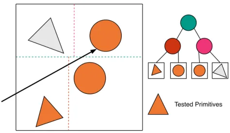
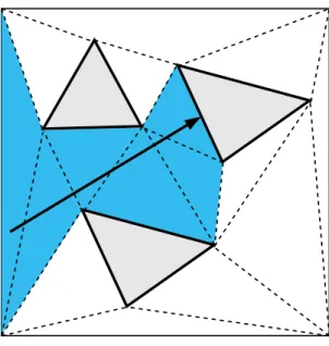
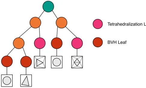
The Bounding Volume Hierarchy-Tetrahedralization Hybrid (BTH) Acceleration structure is composed of a BVH where some leaves of the hierarchy contain tetra-hedralizations of the primitives instead of primitive lists (see Figure 3.1). An axis-aligned bounding box encloses each tetrahedralization leaf node. Traversal in BTH structure is similar to BVH traversal. We recursively traverse each node until we reach a leaf node. In the leaf node, if we have a tetrahedralization, we traverse the tetrahedralization. Otherwise, we check each primitive in the leaf for an intersection. The BTH acceleration structure combines the strengths of BVH and tetrahedralization structures. Compared to BVH, the nearest-hit test on the BTH structure is faster because we can terminate the traversal on tetrahedraliza-tion leaves early. We can construct the BTH structure for the scenes where scenes cannot be completely tetrahedralized. In the BTH structure, a part of the geome-try that can be tetrahedralized can be selected and used as a leaf node. Moreover, the construction of the BTH structure is faster than regular tetrahedralizations due to the non-linear complexity of tetrahedralization algorithms.

(23)

Tetrahedralization Leaf

BVH Leaf

Figure 3.1: Bounding Volume Hierarchy-Tetrahedralization hybrid (BTH) accel-eration structure.

In the following sections, we define construction and nearest-hit traversal meth-ods for the BTH structure.

3.1 Construction

Similar to any hierarchical acceleration structures that are adaptive to the input geometry, the performance of the nearest-hit traversal of BTH depends on the construction quality. Top-Down BTH construction starts with a regular BVH construction. Given input geometry, we construct a BVH using the existing SAH based construction methods. Then, we modify and convert the constructed BVH structure into a BTH structure.

We first construct a complete BVH for the given geometry. Then we select some nodes of the BVH structure to be a tetrahedralization structure. We trim the selected nodes and construct tetrahedralizations for the nodes. We explain the three steps of the top-down construction algorithm (Algorithm 2) as follows:

(24)

Algorithm 2 Top-down BTH construction 1: _{procedure ConstructBthTopDown(primitives)} 2: bvh← ConstructBvhTopDown(primitives) 3: _{MarkSuitableNodes(bvh)} 4: bth← ConstructTetrahedralizations(bvh) 5: return bth

First Step: In the first step, we use the binned BVH construction method [32] to construct a BVH in a top-down fashion. We use the SAH heuristic to build the BVH for the scene.

Second Step: In the second step, we mark the suitable nodes that can be tetrahedralized. Fast tetrahedralization algorithms [23] require self-intersection free geometries as input. Although we can remove self-intersections by splitting the faces and adding new primitives, removing the self-intersections slow down the construction algorithm. Instead, we choose not to tetrahedralize the geometries with self-intersecting primitives. In this step, we mark the BVH nodes that do not contain self-intersecting primitives. We call such nodes as suitable nodes. We mark suitable nodes by a recursive algorithm that visits each node and checks for self-intersection (see Algorithm 3). The algorithm marks the non-self-intersecting nodes starting from the leaf nodes. In leaf nodes, we check each pair of primitives for self-intersection. If a node contains self-intersecting primitives, its parent must also contain the same self-intersecting primitives. Therefore, if a node is marked as unsuitable, its parent is also marked as unsuitable. For an inner node, the algorithm marks the node suitable if the children of the node do not contain any self-intersecting primitives, and the children nodes do not intersect with each other. To detect the collisions between two children nodes, we use the existing BVH structure. The BVH collision test algorithm (see Algorithm 4) checks whether two BVH nodes intersecting with each other [33]. A descend rule is used to determine the node that should be descended first.

We use the BVH we constructed in the previous step to find the self-intersection free nodes. A recursive algorithm marks nodes containing no self-intersecting primitives, starting from the leaf nodes. If a node is a leaf node, we test each

(25)

pair of primitives in the node for self-intersection. If the node is a nonleaf node, it does not contain self-intersecting primitives if and only if both children of the node are non-self-intersecting nodes and the children of the nodes do not intersect with each other.

Algorithm 3 MarkSuitableNodes

1: _{procedure MarkSuitableNodes(node)} 2: if node is a leaf node then

3: if node.primitives has no self intersection then

4: _{MarkSuitable(node)} 5: else 6: l ← node.left child 7: r ← node.right child 8: 9: _{MarkSuitableNodes(l)} 10: _{MarkSuitableNodes(r)} 11:

12: if l and r are suitable then

13: if l.primitives and r.primitives do not intersect then

14: _{MarkSuitable(node)}

Algorithm 4 BVHCollision

1: procedure BVHCollision(node1, node2)

2: _{if !Overlap(node}₁.bounding volume, node2.bounding volume) then

3: return

4: if node1 and node2 are leaf nodes then

5: _{CheckIntersection(node}₁, node2)

6: else

7: if descend node1 then

8: _{BVHCollision(node}₁.left child, node2)

9: _{BVHCollision(node}₁.right child, node2)

10: else

11: _{BVHCollision( node}₁, node2.left child)

12: _{BVHCollision( node}₁, node2.right child)

Third Step: In the last step, we select some of the suitable nodes as tetra-hedralization leaves. Starting from the root node, a recursive algorithm (cf. Al-gorithm 5) traverses the BVH and selects nodes that are advantageous to use as tetrahedralization leaves. Using tetrahedralization nearest-hit cost heuristic,

(26)

Algorithm 5 ConstructTetrahedralizations procedure constructs tetra-hedralizations for advantageous BVH nodes.

1: _{procedure ConstructTetrahedralizations(node)} 2: if node is marked then

3: if Costtet(node) < CostSAH(node) then

4: _Prune(node)

5: _{Tetrahedralize(node.primitives)} 6: return

7: if node is not a leaf node then

8: _{ConstructTetrahedralizations(node.left child)} 9: _{ConstructTetrahedralizations(node.right child)}

we determine whether a node is advantageous to be tetrahedralized or left as a BVH node (cf. Chapter 4). Given a node, if the approximate average nearest-hit cost of traversing tetrahedralization is less than the SAH cost, we select the node as a tetrahedralization node. If a node is selected as a tetrahedralization node, we do not check its children. After the selection process, we convert se-lected BVH nodes into tetrahedralization leaves by pruning their children and constructing tetrahedralizations for the primitives in selected nodes. We use the axis-aligned bounding box of BVH nodes to bound each tetrahedralization. We use Tetgen [23] software to tetrahedralize the primitive groups and use compact tetrahedron representation proposed in [31] to store the tetrahedralizations.

3.2 Traversal

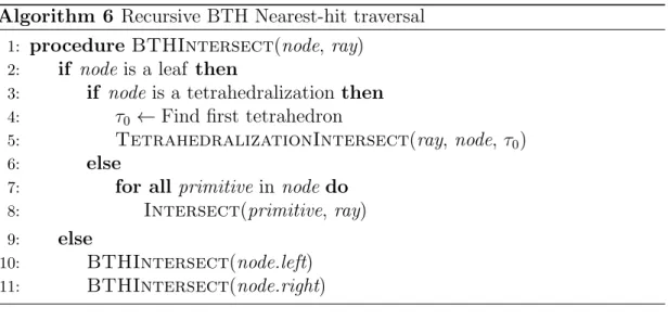
The nearest-hit traversal for the BTH structure (cf. Algorithm 6) is similar to the nearest-hit BVH traversal. Starting from the root, we descent the hierarchy until we reach a leaf node. If the bounding box a node does not intersect with the ray, we do not check its children for an intersection. When we encounter a leaf node, we perform different intersection tests based on the type of the leaf node. If a leaf node does not contain a tetrahedralization, we test for a ray-primitive intersection for all primitives in the node. Otherwise, we traverse the tetrahedralization using the traversal method proposed in [31]. Starting from the initial tetrahedron, we process the tetrahedralization structure, one tetrahedron at a time, until the ray

(27)

hits a primitive face, or it exits the tetrahedralization. Algorithm 6 Recursive BTH Nearest-hit traversal

1: _{procedure BTHIntersect(node, ray)} 2: if node is a leaf then

3: if node is a tetrahedralization then

4: τ₀ ← Find first tetrahedron

5: _{TetrahedralizationIntersect(ray, node, τ}₀)

6: else

7: for all primitive in node do

8: _{Intersect(primitive, ray)} 9: else

10: _{BTHIntersect(node.left)} 11: _{BTHIntersect(node.right)}

Nearest-hit traversal on tetrahedralization requires an initial tetrahedron. If the ray’s origin is inside the boundary of the tetrahedralized area, we use the point-location method explained in [3] to find the tetrahedron that contains the ray’s origin as the initial tetrahedron. If the ray originates from outside the tetrahedralization, we use the faces of the bounding box of the tetrahedralization to find the boundary tetrahedron that the ray first hits. We first locate the point that the ray hits on the boundary (see Figure 3.2). Then we find the face that contains the intersection point. After we find the boundary face, we find the tetrahedron that the face belongs to by using a lookup table.

Figure 3.2: Finding the initial tetrahedron in a bounded tetrahedralization. The initial tetrahedron can be found using the bounding face that the ray hits (shaded region).

(28)

Chapter 4 Tetrahedralization Nearest-Hit

Cost Heuristic

BTH construction algorithm builds tetrahedralizations for nodes that are ad-vantageous to be tetrahedralized. Given a BVH node, the algorithm constructs tetrahedralization for the geometry if the average nearest-hit cost of tetrahedral-ization of the node’s primitives is less than the SAH cost of the corresponding BVH branch (CostT ET(node)< CostSAH(node)). We calculate the approximate

cost assuming

• rays are distributed uniformly throughout the space and • rays originated from the outside of the geometry.

We propose different approximations for the average nearest-hit cost of a tetra-hedralization structure. Since many nodes are considered in BTH construction, a fast cost approximation is essential for quick BTH construction. The approxi-mate nearest-hit cost on tetrahedralization is directly dependent on the number of tetrahedra traversed. We define the approximate cost of traversing a tetrahe-dralization as

(29)

where Ctet is the cost of traversing a single tetrahedron in tetrahedralization,

and Navg(Tnode) is the average number of tetrahedra that are traversed during

nearest-hit traversal for tetrahedralization of the node. To calculate the cost, we first calculate approximation ofNavg(Tnode). Then using Equation 4.1 we calculate

the CostT ET(node). We propose three different ways to approximateNavg(Tnode);

sampling-based cost calculation, average depth-based cost calculation, face count based cost calculation. Among the approximation methods, only the sampling-based calculation requires a tetrahedralization to be present. Others, approximate the cost without requiring a tetrahedralization to be present. For the evaluation of the approximation methods, we used tetrahedralizations of models from the Thingi10k [34] data set.

4.1 Sampling-based Cost Calculation

We calculate the cost using the following Monte Carlo approach; given a tetra-hedralization, we randomly sample rays that originate at the boundary of the tetrahedralization. Then we traverse the tetrahedralization along the ray, count-ing the number of tetrahedra traversed. We calculate the average number of tetrahedra traversed from sampled rays as

Nsampling(Tnode)≈ 1 n n X 0 Nrayi(Tnode) (4.2)

where n is the number of sampled rays and Nrayi(Tnode) is the tetrahedra count

for the randomly sampled ray rayi. With this approach, the accuracy of the

approximated average tetrahedra count gets better as the number of sampled rays increases. Although this approach can approximate the tetrahedra count well, it requires an existing tetrahedralization. Constructing a tetrahedralization for each possible node in the BVH hierarchy is slow and not feasible. We only used this method to evaluate other approximation methods that can approximate the tetrahedra count without requiring a tetrahedralization to be constructed.

(30)

4.2 Average Depth-based Cost Calculation

The average depth-based calculation estimates the average number of tetrahedra traversed during nearest-hit traversal by estimating the average depth of the rays that are sampled on the boundary of the tetrahedralization. The relation between the average ray depth and tetrahedra count is formalized using Theorem 1: Theorem 1. Let s be a line segment starts and ends within the given tetrahe-dralization _{T . s must stab at least} _lksk∗

max tetrahedra of T , where l ∗

max is the length

of longest edge in _{T .}

Ns(T ) ≥ ksk

l∗ max

. (4.3)

Proof. Let τ be a tetrahedron that the line segment intersects. It can be shown that the length of the intersection cannot be greater than lτ

max, wherelτmax is the

length of the longest edge ofτ . Therefore,

ks ∩ τk ≤ lτ

max. (4.4)

By using Equation 4.4 for each tetrahedron that intersects s, we can sum all the lengths, as in Equation 4.5: ksk =X τ ∈T ks ∩ τk ≤X τ ∈T lτ max. (4.5) Since lτ max < l ∗

max for all τ ∈ T from Equation 4.5, we get Equation 4.6.

(31)

(a) Rendering (b) Depth map

Figure 4.1: The average depth estimation using depth map. The elephant model is the courtesy of Qingnan Zhou and Alec Jacobson [34].

By using Theorem 1, we can derive an approximation for the average number of traversed tetrahedra as follows:

Ndepth(Tnode)≈

davg

l∗ avg

, (4.7)

where davg is the average depth of rays in the tetrahedralization and lavg∗ is the

average length of the edges of the constrained faces. To estimate the average depth of rays, davg, we used the z-buffer algorithm to calculate a depth map

(see Figure 4.1) for each side of a bounding box of the constrained faces. The calculation of the depth map with resolutionR requires_O(NR2_{) time complexity}

in the worst case. Using the calculated depth map, we estimated the average depth. Although the depth map only contains the depth of equally spaced axis-aligned rays, it is fast and it can estimate average depth well for most of the models.

Figures 4.2 and 4.3 compare the average depth-based and sampling-based methods. Figure 4.3 shows that the average depth-based cost calculation method underestimates the cost. To resolve this, we modified Equation 4.7 as

Ndepth(Tnode)≈

davg

l∗ avg

(32)

where C is a constant value. 0 100 200 300 400 500

N

sampling 0 100 200 300 400 500

N

depth

Average Depth-based Cost vs Sampling-based Cost

y = x

Average Depth-based Cost

Figure 4.2: The comparison of the estimated tetrahedron count using the average depth-based method and the sampling-based method.

4.3 Primitive Count-based Cost Calculation

In our experiments, we found that the average traversed tetrahedra count is related to the cube root of primitive count. This result is similar to the runtime complexity of regular grids (Θ(√3N )) shown by Clearly and Wyvill [5]. Therefore, we define primitive count-based cost as

(33)

−1 0 1 2 3

Relative Difference (N

depth

− N

sampling

)/N

sampling

0 100 200 300 400

Count

N

depth

Relative Difference (Compared against N

sampling

)

Figure 4.3: The histogram of the relative difference of the tetrahedron count between the average depth-based and sampling-based estimation methods.

(34)

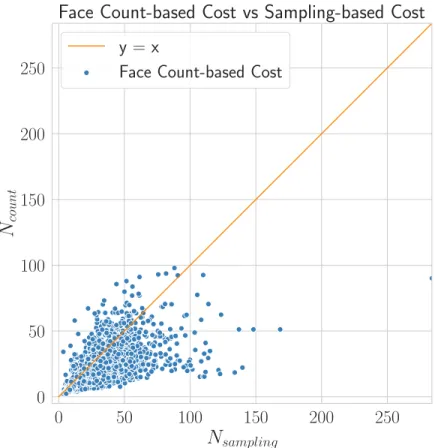
where _{|F | is the number of primitives. Figures 4.4 and 4.5 show the comparison} of primitive count-based method and sampling-based method. It can be seen that the Ncount can approximate the average tetrahedron count well.

0 50 100 150 200 250

N

sampling 0 50 100 150 200 250

N

count

Face Count-based Cost vs Sampling-based Cost

y = x

Face Count-based Cost

Figure 4.4: The comparison of the estimated tetrahedron count using the average depth-based method and the sampling-based method.

(35)

−0.75 −0.50 −0.25 0.00 0.25 0.50 0.75

Relative Difference (N

count

− N

sampling

)/N

sampling

0 50 100 150 200 250 300 350

Count

N

count

Relative Difference (Compared against N

sampling

)

Figure 4.5: The histogram of the relative difference of the tetrahedron count between the primitive count-based and the sampling-based estimation methods.

(36)

Chapter 5 Animated Scenes Using the BTH

Structure

In general, ray tracing acceleration structures are designed for static scenes. For dynamic scenes, acceleration structures need to be adapted. In early research, the effectiveness of acceleration structures only measured using rendering times; the construction costs are usually ignored. As ray tracing achieves interactive frame rates, the construction time is also an issue to be considered as a measure of effectiveness. In general, there is a tradeoff between the construction quality and construction times. For dynamic scenes, both are important because the acceleration structure needs to be updated at each frame.

In terms of dynamic, or animated scenes, there are two approaches to update the acceleration structure when the geometry changes. The first approach is to rebuild the entire acceleration structure. Although rebuilding provides a simple way to adapt to the changing geometry, it can be an expensive operation for some structures. The second approach is to update the existing acceleration structure by only updating parts of the acceleration structure that changed. Although this is more efficient than rebuilding the entire structure, updates reduce the quality of the acceleration structure, thereby reducing the nearest-hit efficiency.

(37)

We can categorize dynamic scenes according to the types of motion that the objects perform. In scenes with hierarchical motion, groups of primitives move in the same way. In incoherent motion, the primitives move independently from each other. Depending on the characterization of motion in the scene different algorithms can be better suited for adapting acceleration structures.

Because BTH structure includes a BVH, most of the dynamic BVH algorithms also work for BTH. The only problem that can arise when adapting a BVH update algorithm into a BTH algorithm is to tetrahedralization leaves. It is shown that a small number of deformations can be applied to tetrahedralizations without any update [3].

We will describe how the BTH structure can be adapted to dynamic scenes that perform hierarchical motions in the following section.

5.1 Two-Level BTH for Hierarchical Motion

If the primitives in the scene exhibit hierarchical motion, we can use two-level (multi-level) hierarchies [35] as an acceleration structure. For such a two-level hierarchy, we group the primitives in the scene into separate objects and build an acceleration structure for each group. Constructed acceleration structures are the bottom-level of the two-level acceleration structure. When building bottom-level acceleration structures, we use the local reference frames of the objects. Then, we construct a top-level acceleration structure for the bottom-level acceleration structures. In two-level hierarchies, nearest-hit traversal starts from the node at the top-level. When we reach a bottom-level node, we transform the ray into the object’s reference frame and test it for intersection using the bottom-level structure. When an object in the scene exhibits a rigid body motion, only the top-level needs to be rebuilt or updated since primitives in the bottom-level acceleration structure does not change. A side effect of level is that two-level acceleration structures also support instancing (see Figure 5.1). When the scene contains duplicate objects, we can use the same bottom-level structure to

(38)

Figure 5.1: An instancing example: Torus knot made of smaller torus knots. Single bottom-level acceleration structure built for one torus knot is enough to render all of the torus knots.

represent the duplicated objects.

We use BVH as the top-level and BTH as the bottom-level acceleration struc-ture for animated scenes (see Figure 5.2). For each object in the 3D scene, we construct a BTH structure. Then we combine these bottom-level structures into the top-level using a BVH. For the construction of BVH, we used the midpoint to partition the bottom-level nodes. In each animation frame, we re-build the top-level BVH using updated coordinates of the objects. The midpoint partitioning scheme allows us to re-build the top-level efficiently for each animation frame.

(39)

Top Level BVH

Bottom Level BTH Bottom Level BTH Bottom Level BTH

(40)

Chapter 6 Experimental Results

6.1 Experimental Setup

Experiments are conducted on a computer with six cores @3.2 GHz (Intel i7-9750H), 16 GB of main memory. We construct the acceleration structures on a single thread. We render images at 1920_{×1080 resolution. For ray tracing, we} used a multi-threaded 16_{×16 tile-based rendering method. For consistency, we} use a single ray per pixel and each ray passes through the center of the pixels in the image plane. We render images using only primary rays without secondary rays or shadow rays.

Our BTH implementations is based on the BVH implementation of Pbrt [36]. We used TetGen [23] tool to tetrahedralize the bounded tetrahedralizations. We used Aman et al.’s [31] Tet32 and Tet20 tetrahedral representation schemes and named our acceleration structures accordingly, i.e., BTH32 and BTH20. Al-though Aman et al. [31] also propose the Tet16 structure, which has a smaller memory requirement than Tet32 and Tet20 structures, we did not use it in our experiments because finding the source tetrahedron that the ray starts in tetra-hedralizations stored by Tet16 scheme requires a more complex lookup table. For comparison, we used BVH and k -d tree implementations of Pbrt.

(41)

In our experiments, we used models from Morgan McGuire’s Computer Graph-ics Archive [37]. Additionally, the Armadillo model is from Krishnamurthy and Levoy [38] and the Crown model is from Martin Lubich [39].

6.2 Selection of Tetrahedralization Cost Method

The average depth-based and the primitive count-based tetrahedralization cost methods allow us to automatically select tetrahedralizations based on their es-timated cost. Both cost estimation methods rely on Ctet, the cost of traversing

a single tetrahedron in tetrahedralization. Different values of Ctet leads to

dif-ferent BTH structures (see Figure 6.1). In general, as Ctet increased, the BTH

construction algorithm selects and constructs fewer tetrahedralizations.

Although we definedCtetas the cost of traversing a single tetrahedron, we used

Ctet as a parameter for the construction of BTH. We performed a grid search on

various models to select the best value for Ctet. We used the construction and

rendering times in Tables 6.1 and 6.2 to select the bestCtet. Because BTH32 and

BTH20 have different tetrahedra traversal times, we decided to selectCtet values

for them separately. For BTH32, we decided to use 0.7 forCtet. For BTH20, we

decided that 0.5 is a good choice for Ctet. Additionally, Tables 6.1 and 6.2 show

the effect of changingCtet. AsCtet increases, more primitives at the leaves of the

BVH structure are tetrahedralized; hence, the construction of the structure takes more time.

We also utilize Tables 6.1 and 6.2 to select the cost method. These tables show that tetrahedralizations built by both average-depth based cost method and primitive count-based cost method can speed-up the rendering times of the BTH structure. Although the calculation of the average depth-based cost method takes more computation time than the primitive count-based cost method, the rendering times of the average depth-based cost method are usually faster than the primitive count-based cost method. In the following experiments, we only use the average depth-based method to construct BTH structures.

(42)

(a) Ctet= 0.1 (b) Ctet = 0.2

(c) Ctet= 0.3 (d) Ctet= 0.4

Figure 6.1: Tetrahedralizations of the BTH structure constructed using different Ctet values. Different tetrahedralizations are colored differently. Gray color is

(43)

Table 6.1: BTH32 statistics for varyingCtet. “No. tet. primitives” is the number

of primitives at the leaf nodes of the BVH that are tetrahedralized. “No. BVH primitives” is the number of primitives at the leaf nodes of the BVH that are not tetrahedralized. Times are in milliseconds (ms).

Primitive count-based cost

Scenes Ctet 0.1 0.3 0.5 0.7 1.0

Armadillo Rendering time 134.34 136.56 86.14 80.43 82.50

Construction time 18,592.1 16,297.3 1,298.2 481.7 479.2

No. tet. primitives 345,938 330,809 30,980 0 0

No. BVH primitives 0 15,129 314,958 345,938 345,938

Lumberyard Rendering time 466.75 492.11 476.28 488.51 477.62

Construction time 6,154.9 4,799.5 3,179.0 2,551.9 1,971.1

No. tet. primitives 119,242 81,051 55,083 32,720 20,121

No. BVH primitives 901,665 939,856 965,824 988,187 1,000,786

Sponza Rendering time 412.98 410.93 408.99 413.85 403.93

Construction time 364.0 361.3 331.2 310.0 307.6

No. BVH primitives 257,503 257,503 260,232 262,267 262,267

Average depth-based cost

Scenes Ctet 0.1 0.3 0.5 0.7 1.0

No. tet. primitives 4,764 4,764 2,035 2,035 0

(44)

Table 6.2: BTH20 statistics for varyingCtet. “No. tet. primitives” is the number

of primitives at the leaf nodes of the BVH that are tetrahedralized. “No. BVH primitives” is the number of primitives at the leaf nodes of the BVH that are not tetrahedralized. Times are in milliseconds (ms).

Primitive count-based cost

Scenes Ctet 0.1 0.3 0.5 0.7 1.0

Construction time 18,882.9 15,812.2 1,302.3 466.3 490.8

No. BVH primitives 901,665 939,856 965,824 988,187 1,000,786

Average depth-based cost

Scenes Ctet 0.1 0.3 0.5 0.7 1.0

Construction time 6,374.3 4,405.2 0 3409.2 2698.6 2329.0

No. tet. primitives 4,764 4,764 2035 2035 0

(45)

6.3 Results

6.3.1 Static Scenes

We used a variety of scenes to compare BTH structure to other acceleration structures. Table 6.3 compare the construction and rendering times our hybrid acceleration structures (BTH32 and BTH20) against other structures (BVHs and k -d trees) for a set of scenes. The scenes in this table cannot be tetrahedral-ized directly. Hence, we did not compare tetrahedralization-based acceleration structures in this table.

Table 6.4 also compare the construction and rendering times our hybrid ac-celeration structures (BTH32 and BTH20) against other acac-celeration structures, including tetrahedralization-based acceleration structures, BVHs and k -d trees, for a set of scenes. The scenes in this table can be directly tetrahedralized without any preprocessing.

In most cases, the BTH structure performs better than the BVH structure This is due to the tetrahedralization traversal cost heuristic. As long as the tetrahedralization traversal cost approximation methods are accurate, the BTH construction algorithm selects the tetrahedralizations that improve the rendering (ray tracing) cost.

For some cases, k -d tree performs better than the BTH structure in terms of the rendering cost. In general, k -d tree performs worse than BTH when the scene contains a large amount of intersecting geometry. Many intersecting ge-ometries cause many duplicate primitives in k -d tree structure. Therefore, self-intersections affect k -d tree negatively, for both construction and rendering times. On the other hand, self-intersections have a small effect on the BTH structure. If a scene contains a high number of self-intersections, these self-intersecting ge-ometry is stored in BVH leaves in the BTH structure.

(46)

In terms of the construction times, compared against BVH, the BTH construc-tion algorithm is always significantly slower than BVH. This can be attributed to the tetrahedralization algorithm. Firstly, TetGen uses algorithms with_O(N2₎

worst-case time complexity. Secondly, robust tetrahedralization with exact arith-metic slows down the tetrahedralization process. In some cases, the BTH struc-ture outperforms the k -d tree. When a scene contains a lot of intersecting geom-etry, the construction of the k -d tree takes a significant amount of computation time. This can be seen in the Hairball model. Since the intersecting geometry is stored in BVH nodes of the BTH structure, BTH performs well.

Compared to tetrahedralizations, rendering using the BTH structure is faster. Besides, the BTH requires less time to construct in all cases than tetrahedraliza-tions. Additionally, another advantage of BTH over tetrahedralizations is that we can build the BTH structure for any three-dimensional geometric models. On the other hand, we can construct tetrahedralizations for non-self-intersecting geometries, or we must perform a self-intersection removal step before tetrahe-dralization.

Experimental results show that the BTH20 has a faster rendering speed than the BTH32. It is because the Tet20 used in BTH20 requires less memory than the Tet32 used in BTH32. The smaller memory requirement of the tetrahedron representation of the BTH20 leads to higher cache utilization than the BTH32. Both the BTH32 and BTH20 structures require approximately similar construct times.

(47)

Table 6.3: The comparison of the construction and rendering times for different acceleration structures on scenes that cannot be directly tetrahedralized. We compare our proposed BTH32 and BTH20 with BVH [36] and k -d tree [36]. Times are in milliseconds (ms).

Scenes

Torus Knot Armadillo Mix Bmw Hairball

No. faces 2,880 345,938 2,505,992 385,162 2,880,000 Rendering times BTH32 14.94 80.09 145.74 92.18 274.73 BTH20 14.66 76.88 140.46 87.73 266.58 BVH 17.50 79.75 145.59 94.36 271.20 k -d tree 15.13 95.09 166.78 88.345 313.78 Construction times BTH32 103.20 496.21 3,558.79 4,293.72 14,527.30 BTH20 101.79 476.33 3,485.51 4,197.93 14,541.70 BVH 2.43 341.56 2,640.36 359.97 2,976.25 k -d tree 24.26 1,459.58 14,127.60 2,489.23 62,846.80 Scenes

Lumberyard Crown Sponza San Miguel Vokselia

No. faces 1,020,907 3,540,310 262,267 9,980,699 1,875,632 Rendering times BTH32 444.60 241.61 378.73 550.58 186.13 BTH20 423.91 231.10 349.98 516.49 173.60 BVH 459.61 242.66 384.20 586.89 190.15 k -d tree 419.74 247.21 213.80 315.46 194.70 Construction times BTH32 2,873.49 24,365.30 1,944.00 18,569.90 4,690.44 BTH20 2,786.16 24,311.90 1,951.73 18,536.50 4,643.17 BVH 1,025.23 3,808.49 245.38 11,185.10 1,546.62 k -d tree 9,315.58 26,292.00 2,028.37 77,815.50 4,521.61

(48)

Table 6.4: The comparison of the construction and rendering times for different acceleration structures on scenes that can be directly tetrahedralized. We com-pare our proposed BTH32 and BTH20 with the tetrahedralization-based acceler-ation structures [31], BVH [36] and k -d tree [36] Times are in milliseconds (ms).

Scenes

Armadillo Mix Mix Close

No. faces 345,938 2,505,992 2,505,992 Rendering times BTH32 79.54 142.37 232.23 BTH20 77.95 140.70 218.13 Tet32 150.84 312.55 363.67 Tet20 118.28 252.76 273.62 BVH 78.71 143.45 224.06 k -d tree 98.18 164.56 254.79 Construction times BTH32 2,398.8 4,473.5 4,593.5 BTH20 3,367.7 4,485.8 4,468.8 Tet32 8,392.1 89,949.7 91,551.4 Tet20 8,380.4 90,291.4 90,564.1 BVH 373.1 2,683.6 2,683.3 k -d tree 1,460.6 14,830.4 14,090.6

(49)

6.3.2 Dynamic Scenes

Figures 6.2, 6.3, and 6.4 show consecutive frames of the animations of the rotating armadillo, the random motion, and the falling hairballs, respectively, rendered using the proposed two-level BVH-BTH structure. We compared the two-level BVH structure against our two-level BVH-BTH structure. Table 6.5 shows the results. In general, the proposed two-level BVH-BTH structure using BTH20 at the lower level is faster than the two-level BVH structure.

Table 6.5: The comparison of the construction and rendering times of different acceleration structures for the animated scenes. We compare the proposed BTH32 and BTH20 with BVH [36]. Times are in milliseconds (ms).

Scenes

Rotating Armadillo Random Motion Falling Hairballs

No. faces 345,938 1,020,907 12,860,699

No. objects 1 101 101

Average rendering times (per frame)

BTH32 70.88 675.51 721.06

BTH20 70.14 659.55 699.02

BVH 70.84 671.56 737.32

Initial Construction times

BTH32 2,403.3 8,831.5 37,920.2

BTH20 2,466.7 9,075.9 38,030.4

(50)

Frame 1 Frame 21

Frame 41 Frame 61

Frame 81 Frame 101

Figure 6.2: Rotating armadillo animated scene rendered using the two-level BVH-BTH structure.

(51)

Frame 1 Frame 21

Frame 41 Frame 61

Frame 81 Frame 101

Figure 6.3: Random motion animated scene rendered using the two-level BVH-BTH structure.

(52)

Frame 1 Frame 21

Frame 40 Frame 61

Frame 81 Frame 101

Figure 6.4: Falling airballs animated scene rendered using the two-level BVH-BTH structure.

(53)

Chapter 7 Conclusions and Future Research

Directions

We proposed the BVH-Tetrahedralization Hybrid structure for accelerating the nearest-hit (ray-surface intersection) tests for the ray tracing algorithm. We tested our acceleration structure with different scenes. Our experiments show that for some of the scenes, our BTH structure outperforms existing acceleration structures. We showed that we could improve the rendering time of the BVH structure by converting it into a BTH hybrid structure. Our experiments show that, in all cases, the proposed BTH20 acceleration structure outperforms the BVH structure in terms of rendering times at the cost of slower construction times. We proposed two methods for approximating average nearest-hit costs for tetrahedralization structures. We show that the proposed cost calculation methods that do not require the construction of tetrahedralizations can provide good approximations for the average nearest-hit cost on tetrahedralized scenes.

Additionally, we can use the two-level acceleration structure for dynamic scenes with hierarchical motions. Our experiments show that the two-level BVH-BTH outperforms the two-level BVH-BVH for the tested scenes where the objects perform hierarchical movements.

(54)

Some possible future work areas can be as follows:

• Adapting the BTH structure for scenes with deforming geometries: One advantage of using tetrahedralizations in the BTH structure is that we can modify tetrahedralizations up to a certain degree without the need for refitting. For animated scenes with deforming geometry, we could use BVH fitting methods to update the BTH structure. We could also use the BTH structure for rendering animated frames of articulated bodies with nonrigid limbs.

• Exploiting ray connectivity for secondary rays: In hierarchical acceleration structures, it is hard to exploit ray connectivity. The nearest-hit test starts from the root of the hierarchy for secondary rays. On the other hand, trac-ing secondary rays is easy on tetrahedralizations. After a primary ray hits a surface, secondary rays can continue from where the primary ray hits with-out the need for an initialization step, which is necessary for tree traversals. Similarly, we can easily trace secondary rays in tetrahedralizations on the leaves of a BTH hierarchy.

(55)

Bibliography

[1] T. Whitted, “An Improved Illumination Model for Shaded Display,” Com-munications of the ACM, vol. 23, p. 343–349, June 1980.

[2] J. T. Kajiya, “The Rendering Equation,” ACM Computer Graphics (Pro-ceedings of SIGGRAPH ’86), vol. 20, p. 143–150, Aug. 1986.

[3] A. Lagae and P. Dutr´e, “Accelerating Ray Tracing using constrained Tetra-hedralizations,” Computer Graphics Forum, vol. 27, no. 4, pp. 1303–1312, 2008.

[4] A. Fujimoto, T. Tanaka, and K. Iwata, “ARTS: Accelerated Ray-tracing System,” in Tutorial: Computer Graphics; Image Synthesis (K. I. Joy, C. W. Grant, N. L. Max, and L. Hatfield, eds.), pp. 148–159, New York, NY, USA: Computer Science Press, Inc., 1988.

[5] J. G. Cleary and G. Wyvill, “Analysis of an Algorithm for Fast Ray Trac-ing UsTrac-ing Uniform Space Subdivision,” The Visual Computer, vol. 4, no. 2, pp. 65–83, 1988.

[6] A. Woo, “Ray Tracing Polygons Using Spatial Subdivision,” in Proceedings of Graphics Interface, vol. 92, (San Francisco, CA, USA), pp. 184–191, Morgan Kaufmann Publishers, Inc., 1992.

[7] K. Klimaszewski and T. W. Sederberg, “Faster Ray Tracing Using Adaptive Grids,” IEEE Computer Graphics and Applications, vol. 17, no. 1, pp. 42–51, 1997.

(56)

[8] T. Ize, P. Shirley, and S. Parker, “Grid Creation Strategies for Efficient Ray Tracing,” in Proceedings of the IEEE Symposium on Interactive Ray Tracing, RT ’07, (Washington, DC, USA), pp. 27–32, IEEE Computer Society, 2007. [9] J. L. Bentley, “Multidimensional Binary Search Trees Used for Associative Searching,” Communications of the ACM, vol. 18, no. 9, pp. 509–517, 1975. [10] J. Goldsmith and J. Salmon, “Automatic Creation of Object Hierarchies for Ray Tracing,” IEEE Computer Graphics and Applications, vol. 7, no. 5, pp. 14–20, 1987.

[11] D. J. MacDonald and K. S. Booth, “Heuristics for Ray Tracing Using Space Subdivision,” The Visual Computer, vol. 6, no. 3, pp. 153–166, 1990.

[12] V. Havran, Heuristic Ray Shooting Algorithms. Ph.d. thesis, Department of Computer Science and Engineering, Faculty of Electrical Engineering, Czech Technical University in Prague, November 2000.

[13] I. Wald and V. Havran, “On Building Fast kd-Trees for Ray Tracing, and on Doing That in O(N log N),” in Proceedings of the IEEE Symposium on Interactive Ray Tracing, pp. 61–69, 2006.

[14] J. H. Clark, “Hierarchical Geometric Models for Visible Surface Algorithms,” Communications of the ACM, vol. 19, no. 10, p. 547–554, 1976.

[15] S. M. Rubin and T. Whitted, “A 3-dimensional Representation for Fast Rendering of Complex Scenes,” ACM Computer Graphics (Proceedings of SIGGRAPH ’80), vol. 14, no. 3, pp. 110–116, 1980.

[16] T. L. Kay and J. T. Kajiya, “Ray Tracing Complex Scenes,” SIGGRAPH Comput. Graph., vol. 20, p. 269–278, Aug. 1986.

[17] G. M¨uller and D. W. Fellner, “Hybrid Scene Structuring with Application to Ray Tracing,” in Proceedings of the International Conference on Visual Computing, pp. 19–26, 1998.

[18] I. Wald, S. Boulos, and P. Shirley, “Ray Tracing Deformable Scenes Using Dynamic Bounding Volume Hierarchies,” ACM Transactions on Graphics, vol. 26, no. 1, Article no. 6, 18 pages, 2007.

(57)

[19] S. Popov, J. Gunther, H.-P. Seidel, and P. Slusallek, “Experiences with streaming construction of sah kd-trees,” in 2006 IEEE Symposium on In-teractive Ray Tracing, pp. 89–94, IEEE, 2006.

[20] I. Wald, “On Fast Construction of SAH-Based Bounding Volume Hierar-chies,” in Proceedings of the IEEE Symposium on Interactive Ray Tracing, RT ’07, pp. 33–40, IEEE, 2007.

[21] B. N. Delaunay, “Sur la Sph`ere Vide,” Izvestia Akademia Nauk SSSR, VII Seria, Otdelenie Matematicheskii i Estestvennyka Nauk, vol. 7, pp. 793–800, 1934.

[22] G. L. Miller, D. Talmor, S.-H. Teng, N. Walkington, and H. Wang, “Control Volume Meshes Using Sphere Packing: Generation, Refinement and Coarsen-ing,” in Proceedings of the 5th International Meshing Roundtable, pp. 47–61, 1996.

[23] H. Si, “TetGen, a Delaunay-Based Quality Tetrahedral Mesh Generator,” ACM Transactions on Mathematical Software, vol. 41, no. 2, Article no. 11, 36 pages, 2015.

[24] P. L. George, F. Hecht, and ´E. Saltel, “Automatic Mesh Generator with Specified Boundary,” Computer Methods in Applied Mechanics and Engi-neering, vol. 92, no. 3, pp. 269–288, 1991.

[25] J. Ruppert, “A Delaunay Refinement Algorithm for Quality 2-Dimensional Mesh Generation,” Journal of Algorithms, vol. 18, no. 3, pp. 548–585, 1995. [26] J. R. Shewchuk, “Tetrahedral Mesh Generation by Delaunay Refinement,” in Proceedings of the Fourteenth Annual Symposium on Computational ge-ometry, SCG ’98, pp. 86–95, 1998.

[27] J. R. Shewchuk, “Adaptive Precision Floating-Point Arithmetic and Fast Ro-bust Geometric Predicates,” Discrete and Computational Geometry, vol. 18, pp. 305–363, 1996.

(58)

[28] Y. Hu, Q. Zhou, X. Gao, A. Jacobson, D. Zorin, and D. Panozzo, “Tetrahe-dral Meshing in the Wild,” ACM Transactions on Graphics, vol. 37, no. 4, Article no. 60, 14 pages, 2018.

[29] Y. Hu, T. Schneider, B. Wang, D. Zorin, and D. Panozzo, “Fast Tetrahe-dral Meshing in the Wild,” ACM Transactions on Graphics, vol. 39, no. 4, Article no. 117, 18 pages, July 2020.

[30] M. Maria, S. Horna, and L. Aveneau, “Efficient Ray Traversal of Constrained Delaunay Tetrahedralization,” in Proceedings of the 12th International Joint Conference on Computer Vision, Imaging and Computer Graphics Theory and Applications, vol. 1 of VISIGRAPP ’17, pp. 236–243, 2017.

[31] A. Aman, S. Demirci, and U. G¨ud¨ukbay, “Compact Tetrahedralization-based Acceleration Structure for Ray Tracing,” Computers & Graphics, Submitted. [32] I. Wald, “On Fast Construction of SAH-based Bounding Volume Hierar-chies,” in Proceedings of the IEEE Symposium on Interactive Ray Tracing, RT ’07, (Washington, DC, USA), pp. 33–40, IEEE Computer Society, 2007. [33] C. Ericson, Real-Time Collision Detection. San Francisco, CA: CRC Press,

2004.

[34] Q. Zhou and A. Jacobson, “Thingi10K: A Dataset of 10,000 3D-Printing Models,” arXiv preprint arXiv:1605.04797, 2016.

[35] J. Lext and T. Akenine-M¨oller, “Towards Rapid Reconstruction for Ani-mated Ray Tracing,” in Proceedings of Eurographics 2001–Short Presenta-tions, pp. 311–318, 2001.

[36] M. Pharr, W. Jakob, and G. Humphreys, Physically Based Rendering: From Theory to Implementation. San Francisco, CA, USA: Morgan Kaufmann Publishers, Inc., 3rd ed., 2016.

[37] M. McGuire, “Computer Graphics Archive,” July 2017.

(59)

[38] V. Krishnamurthy and M. Levoy, “Fitting Smooth Surfaces to Dense Polygon Meshes,” in Proceedings of the 23rd Annual Conference on Computer Graphics and Interactive Techniques, SIGGRAPH ’96, pp. 313–324, 1996.

Bounding volume hierarchy-tetrahedralization hybrid acceleration structure for ray tracing

BOUNDING VOLUME

HIERARCHY-TETRAHEDRALIZATION

HYBRID ACCELERATION STRUCTURE

FOR RAY TRACING

a thesis submitted to

the graduate school of engineering and science

of bilkent university

in partial fulfillment of the requirements for

the degree of

master of science

in

computer engineering

By

Serkan Demirci

December 2020

ABSTRACT

BOUNDING VOLUME

HIERARCHY-TETRAHEDRALIZATION HYBRID

ACCELERATION STRUCTURE FOR RAY TRACING

¨

OZET

IS¸IN ˙IZLEME ˙IC

¸ ˙IN SINIRLAYICI HAC˙IM

H˙IYERARS¸˙IS˙I-D ¨

ORTY ¨

UZLEME H˙IBR˙IT

HIZLANDIRICI YAPISI

Acknowledgement

Contents

List of Figures

List of Tables

Chapter 1

Introduction

1.1

Motivation

1.2

Contributions

1.3

Organization of the Thesis

Chapter 2

Background and Related Work

2.1

Grids

2.2

K -d Trees

2.3

Bounding Volume Hierarchies

2.4

Tetrahedralizations

Chapter 3

Bounding Volume

Hierarchy-Tetrahedralization Hybrid (BTH)

Acceleration Structure

3.1

Construction

3.2

Traversal

Chapter 4

Tetrahedralization Nearest-Hit

Cost Heuristic

4.1

Sampling-based Cost Calculation

4.2

Average Depth-based Cost Calculation

N

N

Average Depth-based Cost vs Sampling-based Cost

4.3

Primitive Count-based Cost Calculation

Relative Difference (N

− N

)/N

Count

N

Relative Difference (Compared against N

)

N

N

Face Count-based Cost vs Sampling-based Cost