Rule based segmentation of colon glands

RULE BASED SEGMENTATION OF COLON

GLANDS

a thesis submitted to

the graduate school of engineering and science

of bilkent university

in partial fulfillment of the requirements for

the degree of

master of science

in

computer engineering

By

Simge Y¨

ucel

September 2018

RULE BASED SEGMENTATION OF COLON GLANDS By Simge Y¨ucel

September 2018

We certify that we have read this thesis and that in our opinion it is fully adequate, in scope and in quality, as a thesis for the degree of Master of Science.

C¸ i˘gdem G¨und¨uz Demir(Advisor)

Can Alkan

Aybar Can Acar

Approved for the Graduate School of Engineering and Science:

Ezhan Kara¸san

ABSTRACT

RULE BASED SEGMENTATION OF COLON GLANDS

Simge Y¨ucel

M.S. in Computer Engineering Advisor: C¸ i˘gdem G¨und¨uz Demir

September 2018

Colon adenocarcinoma, which accounts for more than 90 percent of all colorec-tal cancers, originates from epithelial cells that form colon glands. Thus, for its diagnosis and grading, it is important to examine the distortions in the organi-zations of these epithelial cells, and hence, the deformations in the colon glands. Therefore, localization of the glands within a tissue and quantification of their deformations is essential to develop an automated or a semi-automated decision support system. With this motivation, this thesis proposes a new structural seg-mentation algorithm to detect glands in a histopathological tissue image. This structural algorithm proposes to transform the histopathological image into a new representation by locating a set of primitives using the Voronoi diagram, to gen-erate gland candidates by defining a set of rules on this new representation, and to devise an iterative algorithm that selects a subset of these candidates based on their fitness scores. The main contribution of this thesis is the following: The representation introduced by this proposed algorithm enables us to better encode the colon glands by defining the rules and the fitness scores with respect to the appearance of the glands in a colon tissue. This representation and encoding have not been used by the previous studies. The experimental results of our algo-rithm show that this proposed algoalgo-rithm improves the segmentation results of its pixel-based and structural counterparts without applying any further processing.

Keywords: Histopathological image analysis, gland segmentation, Voronoi dia-gram, structural method.

¨

OZET

KALIN BA ˘

GIRSAK BEZLER˙IN˙IN KURALA

DAYANARAK B ¨

OL ¨

UTLENMES˙I

Simge Y¨ucel

Bilgisayar M¨uhendisli˘gi, Y¨uksek Lisans Tez Danı¸smanı: C¸ i˘gdem G¨und¨uz Demir

Eyl¨ul 2018

T¨um kolorektal kanserlerin y¨uzde doksanından fazlasını olu¸sturan kolon ade-nokarsinomu, kolon bezlerini olu¸sturan epitel h¨ucrelerden kaynak almaktadır. Dolayısıyla, bu kanserin tanı ve derecelendirmesinde, epitel h¨ucrelerin organizasy-onlarındaki bozuklukların, bundan dolayı da kolon bezlerindeki deformasyonların incelenmesi ¨onemlidir. Bu nedenle, kolon dokusundaki bezlerin yerlerinin tespit edilmesi ve deformasyonlarının nicelenmesi, otomatik veya yarı otomatik karar destek sistemlerinin geli¸stirilmesi i¸cin esastır. Bu motivasyonla, bu tez, histopa-tolojik doku g¨or¨unt¨ulerindeki bezleri saptamak i¸cin yeni bir yapısal b¨ol¨utleme algoritması ¨onermektedir. Bu yapısal algoritma, Voronoi diyagramı kullanarak histopatolojik g¨or¨unt¨u ¨uzerinde bir temel ¨o˘ge k¨umesi yerle¸stirmeyi ve bu ¸sekilde g¨or¨unt¨uy¨u yeni bir g¨osterime d¨on¨u¸st¨urmeyi; bu yeni g¨osterim ¨uzerinde kurallar tanımlayarak bez adaylarını ¨uretmeyi; ve uygunluk skorlarına g¨ore bu adaylar arasından alt k¨ume se¸cen tekrarlı bir algoritma tasarlamayı ¨onermektedir. Bu tezin ba¸slıca katkısı; ¨onerilen algoritma ile ortaya konan g¨osterimin, bezlerin kolon dokusundaki g¨or¨un¨umlerine g¨ore kural ve uygunluk skoru tanımlayarak, kolon bezlerinin daha iyi kodlanmasına olanak sa˘glamasıdır. Bu g¨osterim ve kodlama daha ¨onceki ¸calı¸smalarda kullanılmamı¸stır. Algoritmamızın deneysel sonu¸cları, ¨onerilen bu algoritmanın, ek bir i¸slem uygulamadan, piksel tabanlı ve yapısal benzerlerinin b¨ol¨utleme sonu¸clarını iyile¸stirdi˘gini g¨ostermi¸stir.

Anahtar s¨ozc¨ukler : Histopatolojik g¨or¨unt¨u analizi, bez b¨ol¨utlemesi, Voronoi diya-gramı, yapısal y¨ontem.

Acknowledgement

First of all, I would like to thank my advisor C¸ i˘gdem G¨und¨uz Demir for guiding and supporting me through this study. It was an honor for me to work with her. I learned lots of things from her, and without her support, I could not able to complete this study. I also would like to thank my jury members Can Alkan and Aybar Can Acar for their valuable feedback to improve this study.

I owe my deepest gratitude to my parents, Feray and Bilal, and my lovely sister Selin. This thesis would not be possible without their support, help, and patience. I am very lucky to have such a family. I think me and my sister have successfully completed a difficult year for both of us. When we look back, we will remember the Sundays that we study together with a smile.

I would like to indicate my special thanks to Ebru Ate¸s for being a sister to me and making my master days unforgettable. She always supported me in my every decision and most importantly tried to protect me in any case. We had very enjoyable days and I am sure we will add more beautiful memories to the existing ones.

Especially I would like to thank three valuable people. I want to start with Troya C¸ a˘gıl K¨oyl¨u for his endless motivation, friendship, and help through my study. He was a great lab pier and I will never forget his moral support for this year. Secondly, I want to thank Seda G¨ulkesen who became a sister and a friend through my master study. I will never forget the joyful Friday nights that we met for studying. Finally, I want to present my special thanks to ˙Istemi Rahman Bah¸ceci for his great support, especially during the last month of my study. I am very happy to know him personally. He is one of the most virtuous and honest person I have ever met and I hope he will never change.

It has been eight years since I started studying at Bilkent University, and dur-ing this time I met many great people. I would like to thank Cemil Kaan Akyol, Miray Ay¸sen, G¨ulfem Demir, Can Fahrettin Koyuncu, Caner Mercan, Muhsin

vi

Can Orhan, Ali Burak ¨Unal, Ba¸sak ¨Unsal and Muhammed Ali Ye¸silyaprak for their friendship, collaboration, and support. Likewise, I would also like to thank all the professors who make a contribution to my education so far.

I want to thank my team leader, teammates and especially Naciye ¨Ozt¨urk for their understanding and support during this hard year.

Finally, I would like to thank two valuable and highly reputable person. My deepest thanks to our great leader Mustafa Kemal Atat¨urk. If I received this education and became an engineer today as a girl, I owe to him. I also would like to thank the founder of our university dear ˙Ihsan Do˘gramacı for giving importance to science and leaving us such a great educational establishment.

Contents

2.2.1 Pixel Based Methods . . . 9

2.2.2 Structural Methods . . . 14

3 Methodology 17 3.1 Voronoi Representation . . . 18

3.2 Gland Candidate Generation . . . 21

3.2.1 Candidate Set-1 . . . 21

CONTENTS viii

3.3 Iterative Gland Localization . . . 27

3.3.1 Metric Definition . . . 27

3.3.2 Iterative Gland Selection Algorithm . . . 30

4 Experiments 36 4.1 Dataset . . . 36 4.2 Evaluation . . . 37 4.3 Parameter Selection . . . 37 4.4 Results . . . 38 5 Conclusion 47

List of Figures

1.1 Structure of a gland. . . 2

1.2 Sample colon tissue image which contains white gaps. . . 4

2.1 Gland structure. . . 9

2.2 Examples of colon tissues containing gland structures. . . 11

3.1 Steps of our algorithm. . . 19

3.2 Steps of generating the Voronoi representation. . . 20

3.3 White connected components . . . 22

3.4 Connected components generated from nuclear Voronoi polygons. 23 3.5 Illustration for the conversion method. . . 25

3.6 Steps of the candidate set generation. . . 26

3.7 Examples for the eliminated candidates. . . 29

3.8 Candidate examples that share Voronoi polygons. . . 31

LIST OF FIGURES x

3.10 The glands selected by the iterative algorithm. . . 35

4.1 Example results from the training set. . . 40 4.2 Example results from the test set. . . 41

List of Tables

4.1 Quantative results obtained on the training images when n=40. . 42 4.2 Quantative results obtained on the training images when n=60. . 43 4.3 Quantative results obtained on the training images when n=80. . 44 4.4 The results obtained by our method and the pixel-based methods,

for the training set. . . 45 4.5 The results obtained by our method and the pixel-based methods,

for the test set. . . 45 4.6 Results of the object-graph method and our proposed method, for

the training set. . . 46 4.7 Results of the object-graph method and our proposed method, for

Chapter 1

Introduction

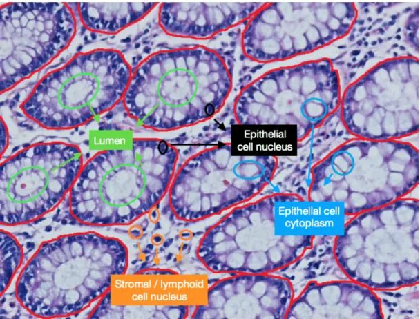
Colorectal cancer is the third most commonly diagnosed cancer type in Western Europe and North America [1, 2]. It is ranked in the fourth place among all cancer-related deaths and 1.1 million deaths are expected by 2030 [3]. The most common type of colorectal cancer is adenocarcinoma, accounting for more than 90 percent of all colorectal cancers. Colon adenocarcinoma originates from epithelial cells, which line up the luminal surface of colon and form colon glands together with the lumina (see Figure 1.1). Thus, for diagnosis and grading of this cancer type, pathologists examine the distortions in the organizations of these epithelial cells, and hence, deformations in the colon glands.

Similar to all cancer types, the colon adenocarcinoma is diagnosed and graded by a histopathological examination of fixed and stained colon tissue sections. In this process, pathologists examine a colon tissue under a microscope and identify whether or not there exist deformations in the glands, and if any, the degree of these deformations. Thus, in order to develop an automated or a semi-automated decision support system, which will help the pathologists make faster and more objective decisions, it is essential to identify gland locations within a tissue and to quantify their deformations. With this motivation, this thesis focuses on the first part, for which it proposes a new gland segmentation algorithm.

Figure 1.1: Sample colon tissue image, on which tissue components are illustrated. Additionally, gland boundaries are drawn with red in the image.

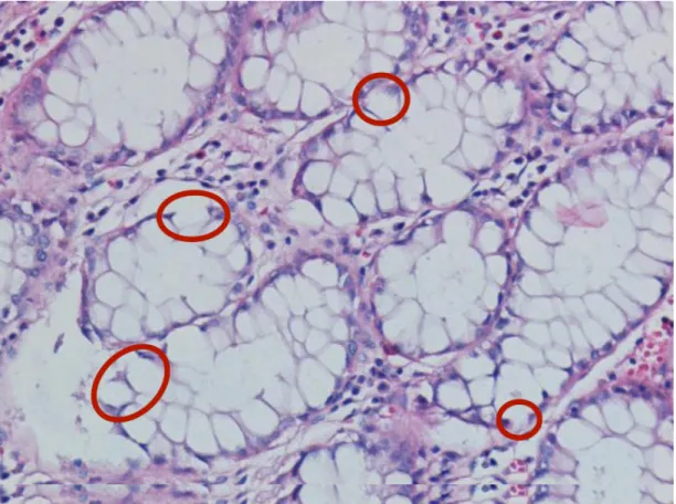
In the literature, the existing gland segmentation methods can mainly be cat-egorized into two: pixel-based and structural methods. The pixel-based methods commonly assign the predefined labels (e.g., nucleus and lumen labels) to image pixels and then apply a post-processing technique on these image labels to form individual glands. These methods indeed rely on the fact that, in a colon tissue image, a typical gland has a large enough whitish luminal region and this region is surrounded by a thick enough line of purplish nuclear pixels. The earlier methods assign labels to the pixels based on their intensities, usually by thresholding [4] or using a simple classifier [5]. On the other hand, these labeling methods may lead to incorrect class labels especially when there exist variations and noise in the pixel intensities. Additionally, the commonly used post-processing techniques (e.g., region growing) applied afterwards may fail when there exist pixel-level variations and imperfections in the gland pixels (e.g., when there exist a consid-erable large white gap in the line of nuclear pixels due to the imperfections in the tissue preparation steps, see Figure 1.2). More recently, the use of deep learning classifiers [6], [7], [8] alleviates the problems related with incorrect pixel labeling. However, they are still prone to the pixel-level imperfections in the image, since they usually require a post-processing step (e.g., applying small area elimination followed by morphological operations) that is applied directly on the pixel la-bels or their probabilities. Additionally, the deep learning methods necessitate a considerable number of annotated images, which sometimes is difficult to obtain. The structural methods typically decompose an image into a set of multi-type primitives (e.g., nuclear and lumen primitives), for instance by locating circles [9] and superpixels [10], and then use the neighborhood information of these primitives to form the glands. Since they run on the primitives (i.e., use the spatial organization of these primitives instead of directly using that of the pixels), these methods are expected to be less susceptible to noise and variations observed at the pixel level (e.g., the one illustrated in Figure 1.2). In this thesis, we propose a new gland segmentation algorithm of this kind.

Figure 1.2: Sample colon tissue image which contains white gaps in between epithelial nuclei due to imperfection in the tissue preparation process.

1.1

Contributions

The proposed algorithm 1.) defines a representation by locating a set of new primitives, 2.) generates gland candidates by defining a set of rules on this repre-sentation according to the spatial distribution of these primitives, and 3.) devises an iterative gland selection algorithm based on the fitness score it proposes.

In particular, the proposed representation decomposes an image into nuclear and white circles, similar to our previous work [9], but then it constructs a Voronoi diagram on the centroids of these circles. Compared to the case where only the circles are used, this Voronoi diagram representation makes easier to define rules for generating the gland candidates, especially when there exist noise and variations.

This thesis defines the gland generation rules and its fitness score, which we call GlandScore, with the motivation of mimicking the appearance of glands in a colon tissue. Particularly, it uses the observations given below. The proposed Voronoi diagram representation facilitates the encoding of these observations as well as the quantification of the fitness measures that they use. These encodings and the definition of their corresponding fitness measures have not been used by the previous methods, and thus, constitute the main contribution of this thesis.

• A colon gland should contain a white luminal region but no nuclei inside. In our representation, this corresponds to finding a large enough connected component of white Voronoi polygons. This component should contain no nuclear polygon inside (or only a few of them when there exist artifacts in the image).

To encode this observation, a gland candidate is formed by identifying each connected component that contains white polygons more than the threshold and combining it with its adjacent nuclear polygons. Then, to quantify the fitness of this candidate, the precision measure is defined as the ratio of the number of the nuclear polygons located on the candidate’s border to the number of all nuclear polygons belonging to the same candidate.

• A colon gland should be surrounded by epithelial nuclei. In our represen-tation, this corresponds to having a row of nuclear Voronoi polygons that confine the white connected component. This connected component should be confined by the nuclear polygons entirely (or only a few of them could be missing when there exist noise in the image).

To encode this observation, a gland candidate is formed similarly. Its fitness is quantified by the recall measure that is defined as the ratio of the number of the nuclear polygons located on the candidate’s border to the number of all polygons (nuclear and white ones) on the same border. Then, by taking the harmonic mean of its precision and recall measures, the Fscore of the candidate is calculated.

• A colon gland should of the tubular shape. In our representation, this corresponds to selecting the compact candidates.

After generating a gland candidate in a similar way, its compactness is quantified by the ConvexRatio measure, which is the ratio of the candidate’s area to that of its convex hull. At the end, for the same gland candidate, all these measures are combined by the GlandScore, which is the product of its Fscore and ConvexRatio measures.

After generating gland candidates and calculating their GlandScores, this the-sis defines an iterative algorithm that selects a subset of these candidates based on their GlandScores. In each iteration, it selects the best candidate and updates the remaining ones that share some polygons with the selected one. This iter-ative algorithm continues until there remains no candidate with a high enough GlandScore.

1.2

Outline

The structure of the remaining of this thesis is as follows. Chapter 2 gives a brief information about the domain and reviews the existing gland segmentation meth-ods in the literature. Then, Chapter 3 provides the details of the proposed gland

segmentation algorithm, explaining its image representation, candidate gland gen-eration, and iterative gland selection steps. This chapter explicitly explains the rules used for gland generation and gives the definitions of the measures used for quantification. Next, Chapter 4 presents experimental settings as well as the results of the proposed algorithm. Finally, Chapter 5 concludes the thesis and presents its future work.

Chapter 2

Background

In the first part of this chapter, we will give general information about glands, their structure, and the staining method. In the second part, we will explicate the existing gland segmentation methods and discuss the feasible and weak sides of these methods.

2.1

Domain Description

The epithelial tissue is made up of glands which produce and secrete hormones, enzymes, and chemical substances that regulate the activity of cells or organs in the body. Glands exist in many different parts of the human body such as lungs, pancreas, and colon. The glands located in colon are in a tubular shape. Fig-ure 2.1 shows the tubular structFig-ure of a gland and FigFig-ure 1.1 explicitly indicates the parts of the glands on a tissue sample [11]. At the center of a gland, there is a big white area which is called lumen. This area is surrounded by columnar epithelial cells. Outer side of these cells, epithelial cell nuclei exist which compose the boundary of a gland. In the stromal part of tissues, stromal cell nuclei are scattered among the glands.

Figure 2.1: Gland structure.

In this thesis, we used images of the colon tissues stained with the hematoxylin-and-eosin (H&E) technique. It is the routinely used staining technique in histopathology. This method stains nucleus with hematoxylin and cytoplasm with eosin [12]. As a result of this staining, the nuclei in images look purple and the cytoplasm and stroma look pink.

2.2

Related Work

Gland segmentation is an important step in the automated or semiautomated detection of colon adenocarcinoma. In the literature, there exist two main ap-proaches to this problem: pixel-based and structural.

2.2.1

Pixel Based Methods

Earlier studies of gland segmentation include pixel-based methods which make use of the intensities of pixels. However, after deep learning, these studies gain another perspective. For this reason, existing pixel-based methods can be cat-egorized into two main classes such as ‘Before Deep Learning’and ‘After Deep Learning’.

Before deep learning, many studies dealt with the gland detection problem by focusing on lumen detection. They utilize the colors’ intensity difference to differentiate luminal and nuclear areas. The study by Wu et al., proposes a method takes an image and applies a simple thresholding to convert it to a binary image [4]. Black parts of the binary image correspond to nuclei and white parts to lumina and cytoplasms. Then, in order to define the initial seeds, big white areas are found, which most probably correspond to the lumina. To find the luminal parts, a window of radius R0 is moved on the image and the white areas,

which completely cover this window, are chosen as potential seeds.

After finding potential seeds, they are expanded by applying iterative morpho-logical dilation operation with a circular structuring element. At each iteration, dilated parts are added to the seed’s area if their pixels are white. The growth of regions is terminated when the pixels reach the nucleus chains. There are some false regions in stroma which form similar structures as glands by growing. In order to prevent the growth of these false regions, an iteration threshold is put and the areas are eliminated if the growth of the region does not stop until this threshold. Then, in order to find the false detected luminal regions, which are not eliminated in the previous step, the thickness of the boundaries are checked by looking at the ratio between the number of nucleus pixels and the number of total pixels on the boundary. If the ratio is very small, this gland is considered false and eliminated.

In another study by Naik et al., a Bayesian classifier is used which classifies pixels based on their intensity values into three classes: nucleus, lumen, and cyto-plasm [5]. Manually labeled pixels are used for training of each class. According to the color values of the training dataset’s pixels, the priors and the probabil-ity densprobabil-ity functions are generated. Then, for each pixel of a given image, the posterior probability of a pixel belonging to a particular class is calculated by using these priors and likelihoods using the Bayes theorem. By thresholding the posterior probabilities with emprically determined values, potential lumen, cyto-plasm, and nuclear regions are detected. From these detected lumens, the ones that are most probably noise are eliminated according to the lumen size, which is defined during the training process by using size histograms. After getting

the possible starting points, a level-set algorithm is performed to find the gland regions. A level-set curve is fitted to the detected lumen areas and the algo-rithm runs until the difference in the contours is below an empirically determined threshold between two iterations. When the difference is higher than this pre-defined threshold, it means that lumen pixels reach to nucleus pixels, and the algorithm stops. The false glands are eliminated by looking at the contours of their boundaries.

Banwari et al. propose a similar study for the purpose of gland segmenta-tion [13]. Their study consists of three steps which are preprocessing, area thresh-olding, and closing. In the preprocessing part, the red channel of the given image is taken and a histogram equalization is applied in order to enhance the contrast. The output of these steps gives the brightest part of the image. Then an average filtering is applied for smoothing the borders of these parts and possible lumen areas are obtained by thresholding according to pixels’ intensities. In the second step of the study, they apply an area thresholding in order to eliminate the small areas. To the remaining areas, the morphological dilation operation is applied. Finally, in the third step, the closing operation is applied to the binary image in order to get the output.

(a) (b) (c)

(d) (e) (f)

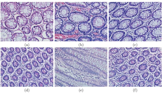
As a result of these studies, it is seen that finding the lumen area, and ex-panding the area with a region growing algorithm is not always appropriate to successfully find glands. These studies use empirically determined area thresholds to distinguish the possible lumen areas from the potential noise. Although this idea may give satisfying results for the images in Figures 2.2 (a), 2.2 (b), and 2.2 (c), it will not give good results for the images in Figures 2.2 (d), 2.2 (e), and 2.2 (f), since their lumen areas are not big enough. Secondly, labeling methods may lead to incorrect class labels especially when there exist variations and noise in the pixel intensities. Also for the same reason, the post-processing techniques (e.g., region growing) may fail on such images.

More recently, researchers start to use deep learning classifiers to alleviate the problems related with incorrect pixel labeling. One of the latest studies by Chen et al. proposes a deep contour-aware network to solve gland segmentation problem [6]. This study uses a fully convolutional neural network for multi-level feature representation. The network takes an image as input and outputs the segmentation probability map and depicted contours of gland objects simulta-neously. The network’s architecture consists of down-sampling and up-sampling paths. First of all, the network down-samples the image with convolutional and max-pooling layers. The results of the down-sampled layers are up-sampled with two different branches to give the segmented object and contour masks separately as outputs. Instead of implementing separate networks for the segmentation of objects and the detection of contours, they design a single network for both pur-poses. Finally, both results are fused together to obtain the final output image. Then, post-processing steps are applied to finalize the resulting image. These steps include small area elimination, smoothing with a disk filter, and filling the holes.

In another study by Manivannan et al., a method is presented which uses exemplar label patches for structure prediction [7]. In the training process, label patches are extracted from the ground truths of the training images. In order to get a set of label exemplars, these patches are clustered with the k-means clustering algorithm. After obtaining K exemplars, linear classifiers are defined for each of them to learn their structures. In the test process, for each pixel

of a given test image, the classifiers output K separate probabilities, each of which corresponds to each exemplar and the pixel is labeled with the one whose probability is the highest. The higher values of the output map indicate the possible gland locations. In order to get glands from the output map, they apply a fixed threshold, which is defined in the training process. Then, for separating the adjacent glands, they apply the morphological erosion operation with a circular structuring element, and after this step, eliminate small connected components. To finalize the result, they apply the morphological dilation operation with a circular structuring element whose radius is twice the size of the structuring element’s radius used in erosion.

Besides all these studies, Xu et al. propose an algorithm for gland segmentation using deep multichannel neural networks [8]. In this approach, they aim to detect the pixels of glands and recognize individual glands at the same time. In the proposed algorithm, they make use of multichannel learning; one channel for foreground segmentation, one channel for edge detection, and one channel for individual gland recognition. The foreground segmentation channel distinguishes glands from the background by using a fully convolutional neural network. The edge detection channel uses a Holistically-nested Edge Detector (HED) to detect boundaries between glands [14]. HED is a convolutional neural network based solution for edge detection. The individual gland recognition channel makes use of Faster Regional CNN (R-CNN) to get location information and Region Proposal Network (RPN) to form the final gland detection result [15]. After receiving the outputs of these three channels, which contain the information about the region, location, and boundary, a fusion algorithm is applied to combine them. In order to fuse these three channels, a convolutional neural network is used. To conclude, four different neural networks are used in this study, three of them for extracting the features, and the remaining one is to combine the outputs of the first three ones.

Although using neural networks for gland segmentation yields promising re-sults, it has the disadvantage of necessitating a considerable number of annotated images and requiring a relatively larger computational time.

2.2.2

Structural Methods

In the literature, there are few studies which handle gland segmentation via struc-tural methods. The common approach of these methods is decomposing the image into primitives and forming gland structures via using the neighborhood infor-mation of these primitives.

Gunduz-Demir et al. present one of the first studies in this field [9]. In the first step of their proposed algorithm, they quantize the image into three clusters (nucleus, stroma, and lumen clusters) by using the k-means algorithm. Then, they locate circular objects on the nucleus and lumen clusters, separately. They construct an object graph on lumen objects, and extract their local features on this graph. For each lumen object, they extract structural features, considering the neighborhood information between this object and its closest nuclear and lumen objects. Then, these features are used to group the lumen objects into two classes as gland and non-gland, by using the k-means algorithm. In the second part of the algorithm, another object-graph is constructed on nucleus circles. Edges are drawn between each nucleus object and its closest objects. Finally, a region growing algorithm is applied to the gland objects. The algorithm stops when a gland structure reaches to the edges of the nucleus-graph. At the end of the region growing process, small regions are eliminated, and a decision tree classifier is used to eliminate false glands.

In another study, Sirinukunwattana et al. propose a Random Polygons Model for modeling glandular structures on images [10]. In this model, first of all, they decompose the image into superpixels by using the Simple Linear Iterative Clus-tering (SLIC) algorithm, and for each superpixel a feature vector is extracted which contains color and texture information [16]. Then, a random forest classi-fier is trained on these features in order to get a glandular probability for each superpixel. By using superpixels’ probabilities, a map is obtained which indicates the glandular probability of each pixel on the image. Then, initial seed areas are obtained by thresholding the probability map, and in order to get more reliable results, the morphological erosion and smoothing operations are applied to these

areas.

In the second part of the algorithm, by applying Otsu’s threshold to the hema-toxylin channel of the image, the approximate locations of nuclei are obtained [17]. On those locations, randomly drawn vertices are located. However, the distance between any two vertices should be at least a pre-defined distance threshold d, otherwise, the vertex is rejected. Then, for each seed area, the closest vertices are found and by drawing edges between these vertices a polygon is obtained. More-over, each seed area is expanded by mexpand pixels from all sides of its boundary.

Finally, the Reversible-Jump Markov Chain Monte Carlo (RJMCMC) method takes the obtained polygons, the vertices which are located on the expanded pix-els of these polygons and the probability map as inputs and outputs a sequence of polygons for each seed area [18]. Among these polygons they use maximum a posteriori polygon to estimate the glandular structure. For the elimination of false glands, they defined two criteria. Firstly, the polygons are eliminated whose number of vertices less than or equal to a pre-defined vertex number. Secondly, if the square root of the polygon’s area is less than or equal to the area threshold, this polygon is also eliminated.

Fu et al. propose an unconventional modeling for gland detection [19]. First of all, they convert the image from the Cartesian space to the polar space. Then, to infer the possible gland boundaries they introduce a random field model. They propose to infer the glands by using the knowledge that they form closed shapes. Their idea is, if they place the co-ordinate’s center inside a gland and then con-vert it to the polar space, they expect to see a line structure in the concon-verted image. According to this idea, if they observe a line this means there is a gland. Therefore, they formulate the gland detection problem as detecting the lines in the polar space.

In the Cartesian space, each point of the given image is subsampled by a circular window with a radius of rmax. Then each window is converted to the

polar space in order to get a polar image. A Conditional Random Fields (CRF) model is defined which consists of random variables X and Y [20]. Each row of the polar image is represented with Xi and they are labeled with Yi where Y

corresponds to the gland’s boundary position at that row. In order to infer Y, a graph is constructed for each Xi. To make an inference from these graphs, two

chain structures are used. To obtain the chain structures, they generate two polar images, one is with θ ranging from 0 to Π and the other is with θ ranging from Π to 2Π. After generating the chain structures, the Viterbi algorithm is applied on each structure to infer the optimal Y [21]. Then, the results are combined with a heuristic method which is presented by them.

In this thesis, a new structural method is proposed for the purpose of gland segmentation. Similar to the existing methods, we obtain structures from our primitives. However, our proposed algorithm enables to encode the appearance of glands by using the predefined gland generation rules and their fitness scores, which have not been used by these previous methods.

Chapter 3

Methodology

Our proposed method transforms a histopathological image into a new represen-tation that allows us to devise an iterative gland localization algorithm. In order to transform the image to this representation, Voronoi diagrams are used which represent the given image’s subregions as Voronoi polygons. In the generation process of these polygons, they are labeled as white and nuclear according to the pixels’ colors that they are placed onto. Then, considering these polygons’ locations relative to each other, a candidate set is generated.

A typical structure of a gland consists of a white area known as lumen, which is surrounded by a black border that corresponds to epithelial cell nuclei. In order to generate a candidate set, connected components on white Voronoi polygons are first found. Then, to mimic the structural organization of a gland, one-row Voronoi polygons are added to each white connected component and candidates are obtained. After getting the one-row added version of the candidates, we select them according to their fitness scores. To quantitatively define this fitness score, the GlandScore metric is introduced.

Our iterative algorithm selects the glands by starting from the one with the highest GlandScore. At each selection, the candidates that share Voronoi poly-gons with the selected candidate are updated. The algorithm stops when there

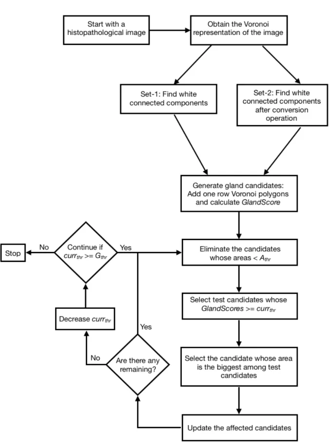
is not any candidate whose GlandScore is higher than the predefined threshold. Figure 3.1 indicates the steps of our proposed algorithm.

3.1

Voronoi Representation

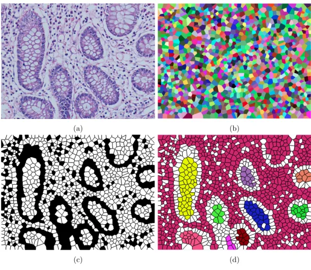
The Voronoi diagram representation of a histopathological image is obtained by following three substeps: pixel labeling, circle localization, and Voronoi diagram construction. For the first substep, a deconvolution operation is first applied to the image, which is stained with the hematoxylin-and-eosin technique [22]. This deconvolution operation is used to emphasize the hematoxylin channel of the given image. Then, the hematoxylin channel of the image is taken and according to this channel’s average intensity value, pixels are divided into two groups. If the intensity value of a pixel is greater than the average, we label the pixel as white, otherwise, we label it as nuclear.

After separating pixels into two groups, the next substep locates circles on each of these groups using the algorithm that was implemented in our research group [23]. In this algorithm, circles are located on the given pixels’ group starting from the largest circle to the one whose radius is at least rmin.

Then the last step takes the centers of these circles and locates a Voronoi diagram onto them. Figure 3.2 indicates the steps of getting the Voronoi repre-sentation for a given image. At the first step, Voronoi polygons are located on the given image. In order to make them more noticeable, each Voronoi polygon is painted with another color in Figure 3.2 (b). The Voronoi polygons are labeled as white and nuclear according to the labels of the circles that they are placed onto. In other words, if a Voronoi polygon is generated for the centroid of a circle which is located on white pixels, then this Voronoi polygon is labeled as white, otherwise, it is labeled as nuclear. Figure 3.2 (c) shows the white and nuclear Voronoi polygons for the given image.

After generating and labeling all Voronoi polygons, white connected compo-nents are found. Figure 3.2 (d) indicates the white connected compocompo-nents. By means of this representation, we are able to define gland candidates easily. In-stead of working on pixels, we use Voronoi polygons and aim to generate possible gland candidates on them.

(a) (b)

(c) (d)

Figure 3.2: Steps of generating the Voronoi representation: (a) Histopathological image, (b) Voronoi diagram of the given image, (c) labeled Voronoi polygons, and (d) connected components generated from white Voronoi polygons.

3.2

Gland Candidate Generation

After getting nuclear and white connected components, we generate gland candi-dates by utilizing this representation. In the ideal case, no gaps should be found in between the Voronoi polygons that correspond to nuclei belonging to a single gland. However, there are some gaps between them and due to this situation we are not able to catch some candidates. Thus, we define two candidate sets, one for the ideal case and the other for the nonideal case. Then, both of these candidate sets are merged before selection.

3.2.1

Candidate Set-1

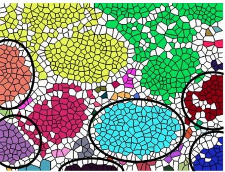
In order to obtain the candidates of the first set, we use the white connected components. Each connected component of this representation acts as a gland candidate. The logic behind directly using the connected components is to catch the glands for the ideal case, in other words, the glands that are successfully separated by nuclear polygons. In Figure 3.3, the connected components which we want to catch are specified with black circles. Note that one row of Voronoi polygons is added to each white connected component since this component only represents the luminal part of a gland but not its epithelial cell nuclei.

3.2.2

Candidate Set-2

The purpose of defining the second set is to obtain the possible gland candidates which are not able to be caught in the first set. For some images especially containing pixel level noise and variations, the connected components generated from white polygons for the first candidate set can output one large component for multiple glands. By defining a rule, we aim to separate these large components to their corresponding glands. These are the candidates for the nonideal case. The green connected component in Figure 3.3 is an example for this case.

Figure 3.3: White connected components which are used in the generation of Candidate Set-1.

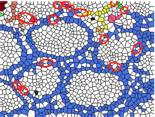
In a tissue image, luminal regions appear as white, as well as some stromal part of the region. Thus, some white regions can exist in between the glands. In order to differentiate white Voronoi polygons that correspond to white regions inside a gland and those in between the multiple glands, white Voronoi polygons are converted to nuclear which are located between nuclear Voronoi polygons. By doing so, we aim to obtain a closed region for the lumen that belongs to a single gland. In Figure 3.4, the places which should be converted are marked with red circles. Afterward, the white connected components are generated on these converted polygons. These white connected components’ one row of Voronoi polygons added versions constitute our second candidate set.

3.2.2.1 Conversion Method for Nuclear Voronoi Polygons

In order to obtain the second candidate set, the white Voronoi polygons which are located between two or more nuclear Voronoi polygons, are converted to nuclear polygons. The reason behind this conversion is that some of the epithelial cell nuclei contain gaps between them. However, we expect that the nuclei belonging

Figure 3.4: This representation shows the connected components which are gen-erated from nuclear Voronoi polygons, for the given image. Red circles indicate the gaps between nuclear polygons, which should be converted.

to an individual gland should be adjacent to each other. Thus, by converting white Voronoi polygons, we aim to fill the gaps which are located on the boundary and obtain a path that includes all nuclear Voronoi polygons of a gland. The important point is that if we converted all of such white Voronoi polygons to nuclear ones, the nuclear connected components would start to close inward of the gland.

In order to minimize this inward closing and prevent unnecessary conversions, we define the following rule: For a white Voronoi polygon, we take its nuclear neighbors which are one step away from this white Voronoi polygon and look at the neighborhood relationships among these neighbors. If all these nuclear neighbors are reachable from each other using only themselves (i.e., if there is a single path among these nuclear neighbors), we do not change the type of this white Voronoi polygon. However, if there is not a path among any of two, the type of the white Voronoi polygon is changed to nuclear in order to obtain a path

among all nuclear Voronoi polygons.

During the conversion process, there is an exceptional case for the white Voronoi polygons which are located on the border of the image. If a white Voronoi polygon, which is on the border, has only one nuclear neighbor that is not on the border of the image, then this white Voronoi polygon is also converted to nuclear. This conversion enables to catch the glands on these locations, by getting closed structures between the nuclear Voronoi polygons and the border of the image.

Figure 3.5 demonstrates two different examples to clarify the conversion method. Figure 3.5 (a) shows the nuclear Voronoi polygons of the given im-age. In this figure, the parts specified with black circles are examined in detail in Figures 3.5 (b) and 3.5 (c). In order to make them more noticeable, all nuclear polygons are shown with blue in Figure 3.5 (b) and the converted polygons are indicated with red in Figure 3.5 (c).

In Figure 3.5 (b), we focus on four different polygons (numbered from 1 to 4) on each selected part. It is seen that Polygon 1 is not converted to nuclear in Figure 3.5 (c) since there is a path between its nuclear neighbors. However, if we separately look at the neighborhood relationships of Polygon 2’s, Polygon 3’s, and Polygon 4’s one step away nuclear Voronoi polygons, it is seen that there is not a single path among them. Therefore, these white Voronoi polygons are converted to nuclear, in order to obtain a continuous path among the nuclear Voronoi polygons on the same white polygon.

After applying the conversion method to the white Voronoi polygons, new white connected components are found. Similar to the first set, one row of Voronoi polygons is added to each of these connected components and they compose of the second candidate set. Figure 3.6 shows the generation process of the candidate sets step by step.

Figure 3 .5: Illustration for the con v ersion metho d. (a) V oronoi p olygons of the n uclear typ e, (b) b efore con v ersion, and (c ) after con v ersion. In (b) and (c), n uclear p olygons are sho wn with blue. The white p olygons that do not chang e their typ es in this con v ersion are sho wn with white whereas those that change their typ es are sho wn with red. H ere the n um b ers in the p o lygons are used in the text for explaining the steps of this con v ersion.

(a) (b)

(c) (d)

(e)

Figure 3.6: Steps of the candidate set generation: (a) Histopathological image, (b) white connected components, (c) nuclear Voronoi polygons before the conversion method, (d) nuclear Voronoi polygons after the conversion method, and (e) white connected components after the conversion operation.

3.3

Iterative Gland Localization

After defining the first and second candidate sets, all candidates are gathered in a single set and the gland selection process is started. In order to differentiate true gland candidates from the false ones, a metric is defined which is called GlandScore. For each candidate, the GlandScore is calculated. Our algorithm selects the candidates iteratively. For each iteration, a current threshold currthr

is used, and the algorithm considers only the candidates whose GlandScores are larger than this threshold. Among these candidates, the one whose area is the biggest is selected and affected candidates’ GlandScores are updated. When there exists no candidate whose GlandScore is greater than currthr, this threshold is

decreased by 0.05 and the same process is repeated. In our method, we start our iterations with currthr=1 and continues until it becomes less than the predefined

threshold Gthr.

3.3.1

Metric Definition

A gland is characterized by a large luminal area surrounded by epithelial cell nuclei. In our representation, the circular white luminal area is represented as a large enough connected component of white Voronoi polygons and epithelial cell nuclei are represented with the connected components of nuclear Voronoi polygons. Thus, a gland in our representation should have an elliptical convex shape. In addition to its shape, the nuclear Voronoi polygons’ distribution is also important. According to our definition, a gland should have enough nuclear Voronoi polygons on its boundary, whereas it does not have much inside.

To mimic the structure of a gland, we define the GlandScore metric. This GlandScore metric is a product of two separate metrics, which are the Con-vexRatio and the Fscore. The first one is the convex ratio which is defined for quantifying the elliptical convex shape. In order to get the ConvexRatio, we use the area and the convex area of a candidate. The second one is the Fscore, which quantifies the nuclear polygons on the boundary and inside of the candidate. The

logic behind defining the Fscore is that the nuclear Voronoi polygons’ ratio both on the boundary and inside of a candidate will give us a value that quantifies the likelihood of that candidate being a gland.

The structure of a gland consists of white Voronoi polygons which are en-circled with nuclear Voronoi polygons. In order to catch the defined structure and approximate the candidates’ closeness to glands, one-row Voronoi polygons is added to white connected components’ boundaries in the candidate generation process. Furthermore, while adding one-row Voronoi polygons, the candidates that contain other candidates inside are eliminated. These correspond to the candidates containing big gaps that another candidate can fit into. However, our glands do not consist of hollow structures, and therefore, those false candidates are directly eliminated at this step. Figure 3.7 shows two different examples for the eliminated candidates.

After obtaining the gland candidates, their GlandScores are calculated ac-cording to the following formulas. For a candidate C, let X(C) be the number of nuclear Voronoi polygons on C ’s boundary, Y(C) be the total number of nuclear Voronoi polygons belonging to C, and Z(C) be the total number of Voronoi poly-gons on C ’s boundary (nuclear as well as white ones). Then, for this candidate C, Precision(C) = X(C) Y(C) (3.1) Recall(C) = X(C) Z(C) (3.2) ConvexRatio(C) = Area(C) ConvexArea(C) (3.3) Fscore(C) = 2 × P recision(C) × Recall(C)

P recision(C) + Recall(C) (3.4) GlandScore(C) = ConvexRatio(C) × F score(C) (3.5)

Note that, when we add one-row Voronoi polygons, the original labels of these polygons are used in the calculation of the GlandScore. This means if a white Voronoi polygon is converted to nuclear during the conversion process, the Gland-Score is calculated by considering the original white label of this polygon.

Figure 3.7: Examples for the eliminated candidates: (a) Histopathological images, (b) candidates of the first set for th e giv en images, (c) eliminated candidates whic h con tain big ga ps that another candidate can fit in to it.

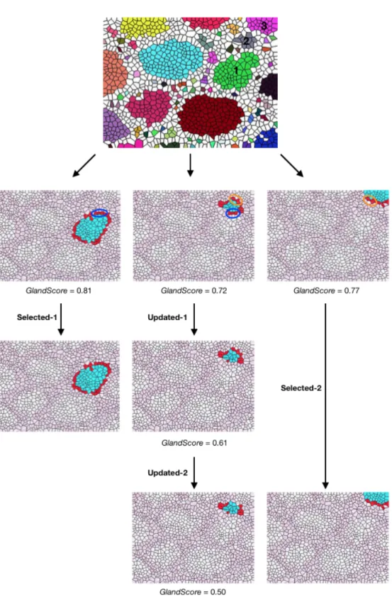
There is an important point that needs to be drawn attention. While adding one-row Voronoi polygons to each candidate’s boundary, some of these Voronoi polygons can be used by more than one candidate. Each candidate’s GlandScore is calculated considering these shared Voronoi polygons. However, in the selec-tion process, the one that is first selected takes the shared Voronoi polygons and these polygons are removed from the other candidates’ structures. As a result, the affected candidates’ GlandScores are recalculated according to the remaining Voronoi polygons. Figure 3.8 shows three candidates that share Voronoi poly-gons. The Voronoi polygons shared by Candidate-1 and Candidate-2 are marked with blue circles, whereas the polygons shared by 2 and Candidate-3 are marked with orange circles. In the GlandScore calculation process, each candidate uses these Voronoi polygons as if they were their own. These can-didates’ calculated GlandScores are indicated under the pictures in Figure 3.8. Among the three of them, Candidate-1 is to be first selected. When it is selected, the Voronoi polygons which are specified with the blue circle are eliminated from Candidate-2 and its GlandScore is recalculated (it drops from 0.72 to 0.61). Then when Candidate-3 is selected, this time Candidate-2 loses the polygons that are indicated with the orange circle and its GlandScore drops to 0.50.

3.3.2

Iterative Gland Selection Algorithm

This algorithm uses an iterative approach to localize the glands based on their GlandScore. After generating candidate sets and calculating each candidate’s GlandScore, our algorithm starts with selecting the “best” candidate according to the GlandScore metric. At each iteration, the affected candidates’ GlandScores are updated. The pseudocode of this procedure is given in Algorithm 1.

Algorithm 1 Iterative Gland Selection Algorithm

Input: candidates C, area threshold Athr, global GlandScore threshold Gthr

Output: detected glands D

1: D = ∅ 2: currthr← 1

// currthr defines a local threshold for each iteration

3: while currthr>= Gthr do

4: while Csubset = {ci ∈ Csubset|GlandScore(ci) >= currthr

5: and area(ci) >= Athr} 6= ∅ do

6: find C∗ ∈ Csubset whose area is largest

7: D = D ∪ C∗ 8: update ∀ci ∈ C

9: end while

10: currthr ← currthr− 0.05

11: end while

Before selection, the candidates whose areas are below a predefined area thresh-old Athr are eliminated. The reason behind this elimination is that, after adding

one-row Voronoi polygons to each white connected component, the GlandScores of some false candidates whose areas are very small become very high. These candidates especially belong to the second set, as a result of the conversions. This elimination prevents our algorithm to be misled by these small white con-nected components. Figure 3.9 shows some eliminated candidates which have been obtained from Candidate Set-2.

In our method, we select Athrto be proportional to the largest area among the

candidates whose GlandScores are higher than the global GlandScore threshold Gthr. The reason of this is the following: Due to the different sizes of each

histopathological image’s glands, defining a fixed Athris not feasible. Thus, at the

beginning of the algorithm, we first find the largest candidate whose GlandScore is higher than the global threshold Gthr and set Athr as the p percent of its area.

Figure 3.9: These are some of the examples which are eliminated through area thresholding. It is seen that their GlandScores are high enough to be considered when one-row of nuclear polygons is added.

the candidates whose GlandScores are greater than or equal to this currthr. (Here

note that Gthr is the global threshold until which the selection continues. On the

other hand, currthr is a local threshold whose value changes among different

iterations.) Among these candidates, our algorithm selects the one whose area is the biggest. This step iteratively continues until all candidates whose GlandScores are greater than or equal to currthr are selected. Then, the local threshold currthr

is decreased by 5 percent. Again, only the candidates whose GlandScores are greater than or equal to the newly set currthr are considered, and the selection is

done similarly. The selection process stops when the value of currthr is less than

the global threshold Gthr. The results of our iterative algorithm are illustrated

on an example image in Figure 3.10.

After each selection, the selected candidate’s Voronoi polygons are eliminated from the others’. Those affected candidates’ GlandScores and areas are recal-culated and updated before the next iteration. Due to these changes, the ones whose areas less than Athr are also eliminated and not considered in the next

iterations. The reason behind using multiple thresholds and decreasing currthr

by 5 percent at each iteration is to give priority to the candidates whose Gland-Scores are greater than a value, and among those, to select the biggest first. If we just considered the area as a criterion and started selecting the one whose area is the largest, candidates whose GlandScores are very high would not be selected at the beginning of the algorithm, because they are small in size even though their GlandScores are high.

When the algorithm stops and returns the detected glands, in order to smooth the shapes of these glands a post-processing step is applied. In this post-processing step, for a gland, its boundary pixels are taken, and from each of the selected pixels, a line is drawn to the nth pixel which comes after itself and the pixels in between the lines of all pixels are included in the gland’s region.

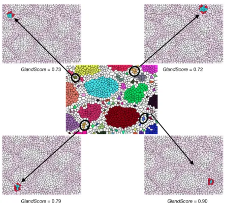
Figure 3.10: The glands selected by the iterative algorithm and their selection order.

Chapter 4

Experiments

In this chapter, firstly we give the details of the dataset that is used for training and testing our algorithm. Secondly, our evaluation technique is described in a detailed way. After the descriptions about the dataset and the evaluation technique, the selected parameters and their ranges are discussed. Finally, the results of our experiments and the results of the existing methods are presented with a discussion about the comparisons between them.

4.1

Dataset

We conduct our experiments on the dataset which contains 72 microscopic images of colon tissues taken from 36 patients. These images are taken from the Pathol-ogy Department Archives of Hacettepe University School of Medicine. They are acquired by a Nikon Coolscope Digital Microscope, by using a 20× microscope objective lens and their resolution is 480 × 640. The first 24 images which are taken from randomly selected 12 patients, constitute the training set. The re-maining 48 images that are taken from the rere-maining 24 patients compose of the test set. All the images in our dataset are stained with the hematoxylin-and-eosin technique.

4.2

Evaluation

We evaluate our segmentation results by using the gold standards of the given images. In the gold standard, foregrounds and backgrounds are annotated. This annotation was performed by our pathologist collaborator.

To quantitatively measure the success of our segmentation method, true posi-tive, false posiposi-tive, true negaposi-tive, and false negative values are calculated at the pixel level. Let A be the gland pixels in the gold standard and C be the gland pixels identified by the algorithm. Then, a pixel P is considered as true positive if P ∈ A and P ∈ C. However, if P ∈ A but P /∈ C, this pixel is considered as false negative. Likewise, P is considered as false positive if P /∈ A but P ∈ C and true negative if P /∈ A and P /∈ C.

Then accuracy, dice index, sensitivity, and specificity evaluation metrics are calculated by using these four values. In particular, they are computed as:

accuracy = T P + T N T P + T N + F P + F N (4.1) dice index = 2 × T P 2 × T P + F P + F N (4.2) sensitivity = T P T P + F N (4.3) specificity = T N T N + F P (4.4)

4.3

Parameter Selection

Our rule based segmentation algorithm has the following four external parame-ters:

• rminis the minimum radius for the circles that are located on the given pixel

as black and white, circles are located on each of these groups starting from the largest circle to the one whose radius is at least rmin. Then, the centers

of these circles are taken and a Voronoi diagram is located onto them. • Gthr is the global GlandScore threshold that we use for the selection of

candidates. Our iterative algorithm starts from currthr = 1. Then, currthr

is decreased by 5 percent at each iteration, until none of the candidates’ GlandScores are greater than or equal to Gthr.

• Athr is the area threshold for the elimination of candidates. Candidates

whose area is smaller than this threshold are eliminated. Since an image may consist of glands of different sizes, defining a fixed Athr for all images

may not be possible. Therefore, for each image, the candidate which has the largest area among the candidates whose glandScore is greater than Gthr is

found. Athr is equal to the p percent of the area of this largest candidate.

• n is the parameter that is used for smoothing the selected glands. At the end of our iterative algorithm, a post-processing step is applied to the selected glands. In this process, the pixels on the boundary are taken for each gland, and a line is drawn from each pixel to the nth pixel which comes after it. At the end, the regions confined with these lines are included to the gland’s region.

These parameteres are obtained using the images of the training set. The ranges of our parameters are as follow: rmin = {3, 4, 5}, Gthr = {0.5, 0.6, 0.7,

0.8}, p = {0.10, 0.15, 0.20}, and n = {40, 60, 80}. Considering all possible combinations of these parameters, we select the combination that gives the highest accuracy on the training set.

4.4

Results

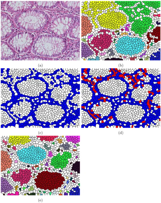
In Figures 4.1 and 4.2, the segmentation results on example images are visually presented. In these figures, the first columns contain original images, the second

columns correspond to their gold standards, and the third columns contain our segmentation results. The images in Figure 4.1 belong to the training set and the ones in Figure 4.2 belong to the test set.

The quantitative results obtained on the training set images are reported in Tables 4.1, 4.2, and 4.3. These tables include the results of all possible combina-tions of the considered parameters. The average performances and their standard deviations are reported and the best results based on accuracy are indicated in bold.

We compare the segmentation results of our algorithm with three different methods. The first two of them are pixel-based methods and the last one is a structural method. Wu et al. present two different pixel-based methods for gland segmentation. In the first study, a region growing algorithm is presented for detecting the glands [4]. In order to find the luminal parts, a window of radius R0is moved on the binary image, which is obtained by thresholding, and the white

areas which completely cover this window are chosen as potential seeds. Then, the seeds are expanded by applying an iterative morphological dilation operation with a circular structuring element. In the second study, a directional filtering based method is presented [24]. They design directional two-dimensional linear filters with different orientations, in order to lower the pixel intensities. For each pixel, the lowest output value of these filters is selected. Then, epithelial cell nuclei are identified by using an intensity threshold. After finding the nucleus pixels the gaps which are surrounded by these pixels are filled with a circular structuring element. The first study approaches gland detection as a lumen-identification problem; on the other hand, the second study approaches it as a nucleus-identification problem.

Both of these methods were previously implemented in our research group. Our proposed algorithm’s and the pixel-based methods’ average quantitative results and their standard deviations are reported in Tables 4.4 and 4.5 for the training and test sets, respectively. According to the results, it is seen that our proposed algorithm improves the segmentation results of these pixel-based algorithms.

(a) (b) (c)

Figure 4.1: Example results from the training set: (a) original images, (b) gold standards of these images, and (c) our segmentation results.

(a) (b) (c)

Figure 4.2: Example results from the test set: (a) original images, (b) gold standards of these images, and (c) our segmentation results.

Table 4.1: Quantative results obtained on the training images when n=40. Av-erage results and their standard deviations are reported.

n = 40 Gthr rmin p 0.5 0.6 0.7 0.8 0.10 accuracy dice index sensitivity specificity 76.14 ± 12.20 76.88 ± 16.31 77.11 ± 20.02 77.01 ± 10.59 78.74 ± 13.09 78.49 ± 16.68 74.93 ± 20.04 85.22 ± 6.87 77.87 ± 16.57 76.44 ± 19.68 69.68 ± 23.48 90.35 ± 6.85 63.57 ± 20.08 49.60 ± 31.90 40.49 ± 31.19 95.81 ± 3.95 3 0.15 accuracy dice index sensitivity specificity 79.24 ± 8.31 80.89 ± 8.95 80.04 ± 12.09 79.22 ± 9.32 81.03 ± 9.82 81.83 ± 9.78 77.34 ± 13.92 86.64 ± 7.08 79.11 ± 14.65 78.23 ± 15.93 70.37 ± 20.44 92.27 ± 5.58 63.31 ± 20.23 48.44 ± 32.71 39.33 ± 31.27 96.80 ± 2.89 0.20 accuracy dice index sensitivity specificity 79.66 ± 8.44 80.58 ± 9.23 77.37 ± 13.04 84.44 ± 8.59 81.22 ± 9.94 81.62 ± 10.07 75.41 ± 14. 08 89.61 ± 6.94 79.07 ± 14.47 78.11 ± 15.83 69.69 ± 20.15 93.40 ± 4.83 62.79 ± 20.62 47.17 ± 33.71 38.30 ± 31.57 97.24 ± 2.76 0.10 accuracy dice index sensitivity specificity 83.19 ± 7.82 85.23 ± 9.04 89.05 ± 11.09 73.91 ± 11.76 85.37 ± 7.10 86.85 ± 8.28 88.49 ± 11.00 79.88 ± 7.83 85.48 ± 9.86 86.75 ± 9.74 85.25 ± 14.26 85.13 ± 7.37 78.34 ± 15.49 77.68 ± 19.48 71.32 ± 22.98 90.45 ± 5.88 4 0.15 accuracy dice index sensitivity specificity 83.43 ± 7.87 84.89 ± 9.97 86.89 ± 12.38 77.90 ± 9.89 85.39 ± 7.50 86.51 ± 9.26 86.22 ± 12.37 82.58 ± 10.02 85.38 ± 9.92 86.28 ± 10.71 83.29 ± 14.92 87.22 ± 8.58 77.22 ± 16.10 75.86 ± 21.53 68.78 ± 23.81 91.54 ± 5.26 0.20 accuracy dice index sensitivity specificity 82.68 ± 9.94 83.84 ± 11.32 83.60 ± 14.93 81.97 ± 8.78 83.99 ± 9.83 84.95 ± 10.89 82.98 ± 14.80 85.17 ± 8.34 84.16 ± 11.45 84.89 ± 12.02 80.76 ± 16.57 88.86 ± 6.41 76.68 ± 16.24 75.18 ± 21.74 67.80 ± 23.88 91.80 ± 5.10 0.10 accuracy dice index sensitivity specificity 72.83 ± 15.59 73.27 ± 18.53 72.22 ± 25.97 75.78 ± 11.77 73.61 ± 16.20 73.77 ± 18.88 71.28 ± 25.44 78.88 ± 10.51 73.96 ± 16.49 73.89 ± 19.30 69.95 ± 24.91 81.18 ± 10.38 70.39 ± 17.57 68.58 ± 22.29 62.05 ± 25.75 85.30 ± 8.17 5 0.15 accuracy dice index sensitivity specificity 75.94 ± 13.31 77.03 ± 16.71 77.43 ± 22.27 73.51 ± 11.56 76.51 ± 13.92 77.32 ± 16.94 75.94 ± 21.70 76.92 ± 11.55 76.48 ± 14.07 77.06 ± 17.11 73.84 ± 21.34 80.12 ± 9.71 70.61 ± 17.27 68.33 ± 22.94 61.55 ± 25.75 86.42 ± 7.84 0.20 accuracy dice index sensitivity specificity 74.96 ± 13.51 75.32 ± 18.14 74.35 ± 23.02 75.61 ± 11.62 75.77 ± 13.92 75.74 ± 18.31 72.91 ± 22.30 79.31 ± 10.63 75.52 ± 14.23 75.31 ± 18.34 70.58 ± 21.70 82.20 ± 9.33 69.43 ± 17.24 66.62 ± 22.67 58.92 ± 25.39 87.52 ± 6.72

Table 4.2: Quantative results obtained on the training images when n=60. Av-erage results and their standard deviations are reported.

n = 60 Gthr rmin p 0.5 0.6 0.7 0.8 0.10 accuracy dice index sensitivity specificity 76.20 ± 12.22 77.18 ± 16.31 76.40 ± 19.77 78.54 ± 9.77 79.09 ± 13.18 78.69 ± 16.74 74.26 ± 19.85 86.38 ± 6.66 77.99 ± 16.64 76.44 ± 19.73 69.06 ± 23.31 91.07 ± 7.03 63.52 ± 20.09 49.38 ± 31.86 39.98 ± 30.81 96.13 ± 3.99 3 0.15 accuracy dice index sensitivity specificity 79.68 ± 8.20 81.15 ± 8.78 79.59 ± 11.78 80.31 ± 8.57 81.26 ± 9.83 81.98 ± 9.74 76.91 ± 13.67 87.36 ± 7.09 79.22 ± 8.20 78.29 ± 15.91 69.95 ± 20.19 92.77 ± 5.69 63.25 ± 20.17 48.27 ± 32.60 38.91 ± 30.87 97.03 ± 2.91 0.20 accuracy dice index sensitivity specificity 79.87 ± 8.35 80.68 ± 9.18 77.07 ± 12.75 84.98 ± 7.84 81.32 ± 9.91 81.67 ± 9.97 75.11 ± 13.84 89.99 ± 6.91 79.09 ± 14.42 78.09 ± 15.76 69.39 ± 19.91 93.66 ± 4.90 62.72 ± 20.55 47.02 ± 33.59 37.98 ± 31.25 97.36 ± 2.84 0.10 accuracy dice index sensitivity specificity 83.35 ± 7.75 85.30 ± 8.99 88.80 ± 11.02 74.47 ± 11.74 85.50 ± 7.04 86.92 ± 8.23 88.26 ± 10.93 80.36 ± 7.86 85.55 ± 9.80 86.77 ± 9.71 84.97 ± 14.12 85.52 ± 7.45 78.34 ± 15.46 77.63 ± 19.48 71.00 ± 22.79 90.78 ± 5.84 4 0.15 accuracy dice index sensitivity specificity 85.53 ± 7.80 84.94 ± 9.90 86.72 ± 12.27 78.25 ± 9.91 85.47 ± 7.43 86.55 ± 9.19 86.04 ± 12.26 82.91 ± 10.01 85.43 ± 9.86 86.29 ± 10.64 83.09 ± 14.78 87.50 ± 8.62 77.23 ± 16.07 75.82 ± 21.49 68.51 ± 23.62 91.82 ± 5.20 0.20 accuracy dice index sensitivity specificity 82.74 ± 9.85 83.86 ± 11.22 83.41 ± 14.77 91.82 ± 5.20 84.05 ± 9.73 84.97 ± 10.79 82.78 ± 14.64 85.46 ± 8.30 84.19 ± 11.39 84.89 ± 11.94 80.55 ± 16.40 89.12 ± 6.45 76.68 ± 16.20 75.14 ± 21.69 67.55 ± 23.68 92.06 ± 5.05 0.10 accuracy dice index sensitivity specificity 72.87 ± 15.61 73.28 ± 18.61 72.08 ± 25.89 75.91 ± 11.71 73.67 ± 16.27 73.78 ± 18.97 71.15 ± 25.37 79.03 ± 10.42 74.02 ± 16.57 73.92 ± 19.38 69.84 ± 24.84 81.35 ± 10.32 70.46 ± 17.64 68.63 ± 22.35 61.93 ± 25.64 85.49 ± 8.13 5 0.15 accuracy dice index sensitivity specificity 75.94 ± 13.34 77.04 ± 16.72 77.33 ± 22.19 73.46 ± 11.77 76.52 ± 13.95 77.33 ± 16.95 75.84 ± 21.62 76.89 ± 11.76 76.51 ± 14.13 77.09 ± 17.16 73.76 ± 21.28 80.15 ± 9.85 70.67 ± 17.34 68.39 ± 22.98 61.47 ± 25.66 86.56 ± 7.81 0.20 accuracy dice index sensitivity specificity 74.97 ± 13.52 75.33 ± 18.14 74.28 ± 22.95 75.54 ± 11.66 75.78 ± 13.52 75.76 ± 18.31 72.85 ± 22.24 79.25 ± 10.77 75.55 ± 14.29 75.35 ± 18.36 70.52 ± 21.65 82.17 ± 9.46 69.49 ± 17.32 66.67 ± 22.71 58.86 ± 25.34 87.60 ± 6.72

Table 4.3: Quantative results obtained on the training images when n=80. Av-erage results and their standard deviations are reported.

n = 80 Gthr rmin p 0.5 0.6 0.7 0.8 0.10 accuracy dice index sensitivity specificity 76.93 ± 12.27 76.97 ± 16.37 74.66 ± 19.82 80.63 ± 9.70 78.99 ± 13.22 78.23 ± 16.83 72.63 ± 19.95 87.76 ± 6.98 77.62 ± 16.59 75.72 ± 19.76 67.58 ± 23.25 91.84 ± 7.12 63.15 ± 19.85 48.52 ± 31.55 38.81 ± 30.09 96.56 ± 3.87 3 0.15 accuracy dice index sensitivity specificity 79.83 ± 8.14 81.02 ± 8.70 78.24 ± 11.81 81.65 ± 8.95 81.12 ± 9.74 81.61 ± 9.71 75.68 ± 13.67 88.09 ± 7.41 78.86 ± 14.48 77.69 ± 15.76 68.75 ± 19.89 93.13 ± 5.81 62.91 ± 19.85 47.61 ± 32.11 37.93 ± 30.05 97.24 ± 2.91 0.20 accuracy dice index sensitivity specificity 80.00 ± 8.26 80.54 ± 9.13 75.83 ± 12.55 86.17 ± 7.15 81.14 ± 9.81 81.26 ± 9.95 73.92 ± 13.71 90.59 ± 7.05 78.76 ± 14.22 77.52 ± 15.58 68.23 ± 19.55 93.99 ± 4.95 62.39 ± 20.22 46.39 ± 33.09 37.05 ± 30.42 97.53 ± 2.86 0.10 accuracy dice index sensitivity specificity 83.53 ± 7.78 85.27 ± 9.09 87.84 ± 11.16 75.90 ± 11.88 85.51 ± 7.07 86.77 ± 8.36 87.33 ± 11.05 81.35 ± 8.09 85.38 ± 9.79 86.46 ± 9.80 84.02 ± 14.09 86.15 ± 7.58 78.14 ± 15.36 77.26 ± 19.39 70.10 ± 22.42 91.27 ± 5.82 4 0.15 accuracy dice index sensitivity specificity 83.55 ± 7.82 84.84 ± 9.97 86.07 ± 12.30 78.92 ± 10.05 85.43 ± 7.46 86.40 ± 9.29 85.41 ± 12.30 83.44 ± 10.14 85.30 ± 9.84 86.07 ± 10.69 82.42 ± 14.69 87.90 ± 8.66 77.11 ± 15.99 75.58 ± 21.40 67.86 ± 23.28 92.24 ± 5.10 0.20 accuracy dice index sensitivity specificity 82.70 ± 9.84 83.73 ± 11.25 82.81 ± 14.66 82.77 ± 8.82 83.98 ± 9.72 84.81 ± 10.83 82.19 ± 14.55 85.89 ± 8.33 84.06 ± 11.36 84.68 ± 11.94 79.92 ± 16.25 89.47 ± 6.49 76.57 ± 16.12 74.93 ± 21.59 66.94 ± 23.32 92.46 ± 4.95 0.10 accuracy dice index sensitivity specificity 72.90 ± 15.68 73.12 ± 18.81 71.47 ± 25.72 76.63 ± 11.44 73.71 ± 16.30 73.64 ± 19.17 70.56 ± 25.20 79.76 ± 10.05 74.04 ± 16.57 73.77 ± 19.53 69.28 ± 24.66 81.98 ± 10.14 70.45 ± 17.62 68.49 ± 22.37 61.42 ± 25.34 85.99 ± 7.82 5 0.15 accuracy dice index sensitivity specificity 75.96 ± 13.36 76.97 ± 16.76 76.92 ± 22.05 73.91 ± 11.66 76.55 ± 13.96 77.27 ± 16.99 75.43 ± 21.47 77.37 ± 11.66 76.55 ± 14.14 77.04 ± 17.21 73.36 ± 21.12 80.63 ± 9.84 70.71 ± 17.35 68.33 ± 22.98 61.11 ± 25.44 87.00 ± 7.48 0.20 accuracy dice index sensitivity specificity 75.00 ± 13.50 75.31 ± 18.13 74.04 ± 22.84 75.84 ± 11.43 75.82 ± 13.93 75.74 ± 18.32 72.60 ± 22.13 79.57 ± 10.59 75.55 ± 14.29 75.33 ± 18.37 70.26 ± 21.53 82.53 ± 9.36 69.53 ± 17.33 66.66 ± 22.72 58.62 ± 25.17 87.96 ± 6.45

Table 4.4: The average results and their standard deviations obtained by our method and the pixel-based methods, for the training set.

Accuracy Dice Index Sensitivity Specificity Our Method 85.55 ± 9.80 86.77 ± 9.71 84.97 ± 14.12 85.52 ± 7.45 Region-Growing [4] 68.58 ± 12.75 56.12 ± 30.54 47.24 ± 29.81 97.70 ± 8.42 Directional Filtering [24] 56.34 ± 18.31 57.27 ± 19.71 55.88 ± 28.48 55.16 ± 32.47

Table 4.5: The average results and their standard deviations obtained by our method and the pixel-based methods, for the test set.

Accuracy Dice Index Sensitivity Specificity Our Method 84.57 ± 8.02 86.05 ± 8.80 84.50 ± 13.28 83.65 ± 7.30 Region-Growing [4] 67.62 ± 17.17 59.04 ± 30.00 52.59 ± 32.88 87.48 ± 15.12 Directional Filtering [24] 53.24 ± 13.62 54.33 ± 19.69 53.77 ± 25.67 51.67 ± 33.64

Secondly, we compare our results with those of the object-graphs method, which was previously developed in our research group [9]. This object-graphs method quantized the given image into three clusters, which correspond to nu-cleus, stroma, and lumen, by using the k-means algorithm. Then, the circle-fit algorithm is applied to fit circles on the nucleus and lumen clusters, separately. An object graph is constructed on lumen objects, by considering nucleus and lumen objects as nodes by drawing edges between each lumen object and its clos-est nuclear and lumen objects. Then, structural features are extracted for each lumen object, by taking advantage of the edges which are drawn in the graph construction process. According to these features, lumen objects are grouped into two classes as gland and non-gland, by using the k-means algorithm. Fur-thermore, another object graph is constructed on nucleus objects and edges are drawn between each nucleus object and its closest objects. Then, a region grow-ing algorithm is applied to the gland objects. The algorithm stops when a gland structure reaches to the edges of the nucleus-graph. Finally, small regions are eliminated, and a decision tree classifier is used to eliminate false glands.