Cutoff rate for fixed-composition on-off keying over direct detection photon channels

(1)

■' vCP’

О V B .- i

■•4!J i~*''fn.f‘· '■&!X,r'-fTT ,· n ;·■' ·< ! -ν'ί„·ΐ Tí ■··“:. í ? A

Z 6 8

f T é S i t e á o

(2)

CUTOFF RATE FOR

FIXED-COM POSITION ON-OFF KEYING

OVER

DIRECT DETECTION PHOTON CHANNELS

A T H E S IS S U B M IT T E D T O T H E D E P A R T M E N T O F E L E C T R IC A L A N D E L E C T R O N IC S En g i n e e r i n g A N D T H E I N S T I T U T E O F E N G IN E E R IN G A N D S C IE N C E S O F B IL K E N T U N IV E R S I T Y IN P A R T IA L F U L F I L L M E N T O F T H E R E Q U IR E M E N T S F O R T H E D E G R E E O F M A S T E R O F S C IE N C E By M. Şenol Toygar June 1990

(3)

Ж '. ί' о Z

-T, ^

* ' '> ·>·

(4)

I certify that I have read this thesis and that, in my opinion, it is fully adequate, in scope and in quality, as a thesis for the degree of Master of Science.

Associate Prof. Dr. Erdal Arikan (Principal Advisor)

I certify that I have read this thesis and that, in my opinion, it is fully adequate, in scope and in quality, as a thesis for the degree of Master of Science.

Assistant Prof. Dr. Gürhan Şaplakoğlu

Approved for the l^istUute of Engineering and. Sciences: ' < / c c C

Prof. Dr. Mehmet Bar ay

Director of Institute of Engineering and Sciences

(5)

(6)

In this thesis, we consider direct detection photon channel with peak and average power constraints. This channel is modelled as a binary input discrete memoryless channel. We study the cutoiFrate for different modulation formats on this channel since it is a measure of decoding complexity when sequential decoding is used and also, it gives an upper bound for the probability of error which decreases exponentially with the constraint length of convolutional code.

Cutoff rates for the ensembles of fixed-composition and independent-letters codes along with ON-OFF keying are computed numerically and also some bounds are given. Curoff rates versus signal-to-noise ratio or peak power are plotted for blocklengths of

N = 40,100 and for both ensembles.

Comparison of cutoff rates for these two ensembles shows that for the direct detec tion photon channel the cutoff rate of ñxed-composition ensemble is signihcantly greater than that of independent-letters ensemble for small values of signal-to-noise ratio and when the average power is a small fraction of peak power, say, 5-30%.

In an uncoded system, for achieving a probability of error P( E) — 10“ ^, we

should send 10 pliotons/slot with rate R = I bit/slot, resulting in an efficiency of 0.1

bits/photon. However, using coding we can make prol)ability of error arbitrarily siiia.il achieving an efficiency of 1 bit/photon.

Also, some remarks on the implementation of fixed-composition trellis codes and on multi-level signalling instead of ON-OFF keying are given in conclusions.

(9)

Ö Z E T

DOĞRUDAN SAPTAMALI FOTON KANALLARINDA

SABİT BİLEŞİMLİ AÇ-KAPA ANAHTARLAMA İÇİN KESİLİM HIZI

M. Şenol Toygar

Elektrik ve Elektronik Mühendisliği Bölümü Yüksek Lisans Tez Yöneticisi: Doç. Dr. Erdal Arıkan

Haziran, 1990

Bu tez çalışmasında, doğrudan saptamalı foton kanalı tepe ve ortalama güç kısıtla maları altında incelenmiştir. Bu kanal iki seviyeli bir girişe sahip ayırtık, belleksiz kanal olarak modellenmiştir. Bundan sonra, dizinsel çözümleme teknikleri kullanıldığında çözümleme güçlüğünün bir ölçütü olması ve evrimsel kodun kısıtlama uzunluğu ile üssel olarak azalan hata olasılığı üst sınırını belirlediğinden, kesilme hızı parametresi bu kanal modeli üzerinde değişik modülasyon formatları için incelenmiştir.

Kesilim hızları, sabit bileşimli ve bağımsız harfli kod toplulukları için AÇ-KAPA anahtarlama tekniği göz önünde tutularak sayısal olarak hesaplanmış ve aynı zamanda bazı alt ve üst sınır ifadeleri verilmiştir. Her iki kod topluluğu ve iki farklı blok uzun luğu {N = 40,100) için sinyal gürültü oranı veya tepe güç değerine karşı kesilim lıızı

çizilmiştir.

Bu iki kod topluluğu için, kesilim hızlarının karşılaştırılması göstermiştir ki, sinyal gürültü oranının düşük değerlerinde ve ortalama güç değerinin tepe güç değerinin küçük bir kesri olduğu zaman (%5-30), sabit bileşimli kod topluluğunun kesilim hızı bağımsız harfli kod topluluğunun kesilim hiindan oldukça büyüktür.

Kodsuz bir sistemde, 10“ ^’luk bir hata olasılığına ulaşalıilmek için, her aralıkta 1 bit için 10 foton yollamamız gerekir; buda foton başına 0.1 b it/foton ’lıık verimlilik sağlamaktadır. Halbuki, kod kullanarak istenildiği kadar küçük hata olasılığına u- laşabiliriz ve hala hazırda 1 bit/foton gibi yüksek bir verimlilik elde edebiliriz.

Ayrıca, sonuç bölümünde sabit bileşimli kafes kodlarının gerçekleştirilmesi ve A.Ç-

KAPA anahtaricima yerine çok seviyeli sinyalleme tekniğinin kullanılması ile ilgili l)azı açıklamalara yer verilmiştir.

Anahtar sözcükler: Kesilim hızı, sabit bileşimli kodlar, foton kanalı, AÇ-KAPA anahtarlama

(10)

A C K N O W L E D G E M E N T

I am grateful to Assoc. Prof. Dr. Erdal Arikcvn for his invaluable guidance and suggestions during the development of this study. My special thanks are due to Prof. Dr. Abdullah Atalar who helped me very much by his encouragement. It is also my pleasure to express my thanks to my friends who assisted in the editing or made life easier with their suggestions.

(11)

Nomenclature

7 Threshold for ML receiver

6,8 Cross-over probabilities for binary DMC

Roi Cutoff rate for independent-letters ensemble

Rofc Cutoff rate for fixed-composition ensemble

4 ^ \ Qn) , Ro Cutoff rate

a Improvement factor in cutoff rate

z Channel parameter which is — ¿) -f \/(5

^0 Dark current level

Qn Input probability distribution -Pw(y|x) Channel transition probabilities

A Slot length

A Peak power level

SNR peak signal-to-noise ratio

UB Upper bound

LB Lower bound

f)

(12)

Chapter 1

INTRODUCTION

In this chapter, direct detection photon channel is described. Capacity, cutoff rate, Rq, and sequential decoding concepts with a brief review of previous work are given.

1.1 Direct Detection Photon Channel

The channel input is a waveform A(i), 0 < t < oo, which satisfies 0 < A(t) < A

where the parameter A is called the peak power. The waveform A(·) defines a pois

son counting process i/{t) with rate A(i) + Aq, where Aq > 0 is the dark current level (background noise). Thus, the statistics for i/(i) can be written as

1^(0) = 0 + r) - u{t) = j ) = where A j! rt+T , j — 0, 1, 2,... 0 < r ,i < oo

= ^ "(A(s) + Ao)

ds

Jumps in !/(·) correspond to photon arrivals at the receiver and they can he determined

by using a photon detector.

For a set of M messages, Xm(t) is sent for message m, I < m < M , where Xmit)

is nonzero only for 0 < / < T where T is the signalling interval. In addition to the peak

power constraint, these waveforms also satisfy the average power constraint r T

(13)

(Actually, for the codes we consider this condition will always hold with equality.)

Shannon [1] proved that there is a parameter C, called channel capacity which is the maximum of achievable rates allowing reliable communication. This capacity incorporates the effects of noise, constrained bandwidth and power limitations related to any physical channel. The significance of channel capacity can be stated as follows If there are M = messages for some fixed i2, called the rate of the code, then:

• arbitrarily small error probability can be obtained for T large enough if R < C .

• the probability of error must go to 1 as T increases if ii > C.

Shannon did not, however, tell how to find suitable codes to construct a reliable system which works at rates close to channel capacity; his achievement was to prove only the existence of such codes. Since then, major part of the communication research has been devoted to extend these results and achieve rates closer to the channel capacity.

1.2 R

q

and Sequential Decoding

C H A P T E R !. INTRODUCTION 2

The aim of this thesis is to study the Rq parameter for various modulation formats on the direct detection photon channel. The motivation for using the Rq parameter as a criterion for comparing different coding and modulation schemes arises from using trellis coding along with sequential decoding. Wozencraft and Kennedy [2] argued in favor of the cutoff rate as a criterion because it is the upper limit of code rates R for which the

average decoding computation per source digit is finite when sequential decoding is used. Viterbi [3] showed, for convolutional coding and maximum likelihood decoding on the discrete memoryless channel (DM C), that the error probability is upper l)ounded by

P{E) < CrLc- ’^ ^ li R < Ro

where N is the constraint length of the convolutional code, R is the code rate, L is the

total number of source letters encoded, and Cr is a weakly dependent function of R and

not a function of L or N. Thus, the single parameter Rq provides a measure of both reliable rates and code complexity.

So, if the communication rate is less than Rq^ it is possible to construct sequential

decoders that have error probability approaching zero exponentially by increasing the constraint length N of the trellis code.

^Note that M = and without loss of generality blocklength N = ^ can be replaced by T, where A is bit interval.

(14)

1.3 Brief Review of Previous Work

Snyder et. al. [5] examined cutoff rate as a performance measure in the design of encoder, optical modulator and demodulator of the direct detection photon channel. Channel is modelled as a memoryless channel with continuous output alphabet that corresponds to the limiting case of infinitely fine quantization. Davis [6] computed the capacity of a Poisson-type channel subject to peak amplitude and average energy constraints. In [11] capacity and error exponent of the direct detection photon channel is calculated, and an explicit construction for an exponentially optimum family of codes for this channel is given. In [7] and [8], assuming a noiseless photon channel, capacity and cutoff rate are calculated. While capacity can be made arbitrarily large, cutoff rate is bounded,

Ro < 1. Also, some codes are discussed in these papers. Pulse position modulation

(PPM ) for noiseless photon channel is examined by Zwillinger [10] and Bar-David et. al. [9] considering capacity and cutoff rate. Georghiades [12] showed how trellis coded modulation can be used to improve the performance of the direct detection photon channel. Forestieri et. al. [13] studied the performance of convolutional codes in this channel.

CHAPTER 1. INTRODUCTION 3

1.4 Summary of Results

The work in this thesis differs from the previous work in that here an ensemble of fixed- composition codes along with ON-OFF keying is considered. The cutoff rate parameter for the resulting channel is computed numerically and asymptotic bounds are given. The results demonstrate that significant coding gains are achievable by using fixed- composition ensembles of codes (rather than the more commonly used independent- letters ensemble).

(15)

Chapter 2 Ro

A N A L Y S IS F O R

F IX E D -C O M P O S IT IO N A N D

IN D E P E N D E N T -L E T T E R S

E N SE M B LE S

2.1 Discrete-time Photon Channel

Consider the direct detection photon channel described in Section 1.1. Let signalling interval [0,T] be divided into N slots. Let A be the slot length

T

A =

N'

Consider ON-OFF signalling on this slotted channel. That is, denote message m by a

binary vector Xm = {xmi,Xm2·, · ■ · ,Xw,n)·, Xmi = 0,1 and let the corresponding signal

waveform be given by

= XmnA for (n - 1)A < t < nA n = 1, 2,...,iV.

Thus, Xm{t) takes only the values A or 0 in the bit interval (slot) ( ( n - l ) A , n A ] according

as Xmn is 1 or 0, respectively. We assume that the receiver is an ML decoder which bases

its decisions on the increments

yn = i^(nA) — u{{n — 1)A ) , where i/(0) = 0.

That is, the receiver decides that the bit value in the n’th time slot was a 1 if PiVnl^mn ~ 1) ^ P{,yn\X'mn ~ 0)

0 if P{yn\Xmn = 0) > P{yn\Xmn = 1)·

We have

P{j\i)

=

P{yn

=

j\xmn = i )=

" -.r'^· ,

i = 0,1

(16)

r-CHAPTER 2. Ro ANALYSIS FOR FC AND IL ENSEMBLES where Ao = / (0 + Aq) ds = AqA J (n—1) A rnA Ai = / (A + Aq) ds = (A + Ao)A. J(n-1)A Hence, Pfalo) ■ VAo7

So, the receiver decides that a 1 was sent if and only if the number of received photons,

j , exceeds the threshold 7 , where

_ Ai — Aq _______________

I n (^ ) ~ \ n ( l + SNR)— --- , S N R = ^ }

_A

q

(2.1)

As a result, the slotted direct detection photon channel with ON-OFF keying can be modelled as a DMC with the following cross-over probabilities

g-(4-|-Ao)Aj(^^ Ao)A]^' £ = F (0|1) = x ; 6 = p ( i i o ) = x : i>7 e-^o^(AoA)> 1 - e (2.2)

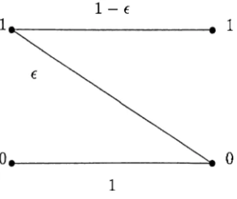
Figure 2.1: Binary DMC model for the direct detection photon channel

In the case of Aq = 0 (no dark current), the above DMC becomes a Z-channel with

S = 0 (Figure 2.2)

' Actually this should be defined as peak signal-to-noise ratio, but for simplicity it will be refered as SNR througout the text.

(17)

CHAPTER 2. Ro ANALYSIS FOR FC AND IL ENSEMBLES

1 - €

Figure 2.2: Z-channel model for the direct detection photon channel in the case of Aq = 0

2.2 Calculation of Cutoff Rates

Consider a code ensemble of blocklength N over an alphabet A. Thus, each word in

the ensemble belongs to and there is a probability distribution Qat defined on A ^ .

Qtv(x) is then the probability of x being chosen as a codeword. We let P7v(y|x) denote

the probability that the channel output block y = (2/i> 2/2? · · · ? 2/n) is received when the channel input block x = (x‘i,x’29 · · · is transmitted. For a DMC, Pj^{y\x) =

The cutoff rate parameter for the above ensemble and associated channel is defined by [4, p.l35]

4 ^ \ Q N ) = - j ^ l n (^X ^<3N (x)\/iV (ylx)j (2.3)

The goal is to maximize this parameter by variation of Qm and N subject to certain

constraints on the code ensemble such as peak or average power constraints. This leads to the definition

(2.4)

Ro = sup maxi?i^V<5Ar) 7V>1 Qn

where for each N, varies over probability distributions satisfying the constraints.

(18)

CHAPTER 2. Ro ANALYSIS FOR FC AND IL ENSEMBLES

2.2.1 Independent-Letters Ensemble

For an independent-letters ensemble over a binary alphabet A = { 0, 1}, the probability

of choosing X as a codeword has a product form:

N

1=1

where n i(x ) and no(x) are the number of I ’s and O’s respectively in x G . That is,

each letter o f each codeword is chosen independently. Using Equations 2.4 and 2.3, Ro

for independent-letters ensemble can be calculated as follows:

Y (YQN{^)\/PN{y\y^)] = IZLI3'5iv(x)Q N(x')\/-fV(y|x)T’N(ylx')

y X X N

= ïl'LT,JLQMQ{<)^/P(yiMP(κK)

1=1 Vi Xi xj 1 1 1 HN i z i z Qiî)Qiî)\/Piyi\î)PiyiWi) _Î/1=0 xi=0x'=0 + ( 1 - p f + 2j){l - p){^c{\ - S) 4- y (5(1 - e))

Thus, the supremum over N in Equation 2.4 is achieved at iV = 1 for this

ensemble, and cutoff rate for independent-letters ensemble, Roi is given by

Roi = sup m axR ^ \ Qn) = max — Inip^ + (1 — PŸ + 2p (l — p)z] (2.5)

N>1 Qn p

where

z — y ^ c(l - (5) 4-

\J

(5(1 — e) (2.6)

and the maximum over p must be carried out subject to power constraints, if there are

any. As Equation 2.5 implies, we gain nothing by increasing the blocklength, N, for

independent-letters ensembles.

2.2.2 Fixed-Composition Ensemble

Each codeword from the ensemble of fixed-composition codes has the same fixed number

K of I ’s. Thus, if the blocklength is N then we have

(19)

words in the ensemble. We choose codewords from this ensemble with probability dis tribution

Q

n

(

x

) =

CHAPTER 2, Ro ANALYSIS FOR FC AND IL ENSEMBLES 8

N K

Cutoff rate for the fixed-composition ensemble, i^o/c? can be calculated as follows.

= E E

EE ■

■

E n

X X ' y\ V2 Vn 1 = 1

= J2J2

qn{^)Qn

{^') n E yjp(.y,\^i)p{yi\x'd

X X' z=l Vi

if Xi = x'i then ^ yjP(yi\xi)P{yi\x'{) = ^ P{yi\xi) = 1

Vi Vi

if Xi 7^ æ· then ^ ^Jp{yi\xi)P{yi\x'^) = ^€{1 - 6) + ^ 6 { l - e)

Vi

Therefore,

X X'

where d (x ,x ') is the distance between the codewords x and x ' which is defined as the number of bits where one codeword differs from the other one, and 2: is given by Equation

2.6.

, - « < > ( « » ) = e < 3 « ( = '') Ec« ( ’‘ )^''‘ ’‘ '’‘ '’

X ' X

for any x ' inner summation will be the same, so we can write

N N K

Y^Nd{xo)z'^ (2.7)

¿=0

where M is the total number of the codewords for the fixed-composition ensemble and Nd(xo) is the number of the codewords that are at distance d from the codeword xq.

Thus,

/

\

^ E

(2-8)

N \ j=o

(20)

CHAPTER 2. Ro ANALYSIS FOR FC AND IL ENSEMBLES

Nd(xo) =

d is odd d > 2K

d is even and d < 2K

where it is assumed that K < Therefore, N — K > K, Unlike to the independent-

letters ensemble, here we have the possibility to increase Rq by increasing blocklength,

N, This result is demonstrated in Section 2.3.

2.3 Comparison of Cutoff Rates

For a fair comparison of the two ensembles, we take K = j?N, and compute the cutoff

rates as a function of p and N. Thus, for the independent-letters ensemble an average

number of N AAp photons are sent per codeword; for the ñxed-composition ensemble

exactly N AAp photons are sent per codeword.

For the independent-letters ensemble Rq does not depend on N ^ but for the fixed-

composition ensemble it improves as N is increased. The main point we wish to demon

strate is that the fixed-composition ensemble has a significantly larger Rq than the independent-letters ensemble.

Cross over probabilities (e and 6) for the DMC in Figures 2.1 and 2.2 depend

on the signal-to-noise ratio ( SNR = and also on AA (photons/slot) which is the

number of photons per bit interval. For .4A = 2,5,10,50 various plots of Rq versus

SNR are given with the parameter p changing from 0.05 to 0.50 by increments of 0.05

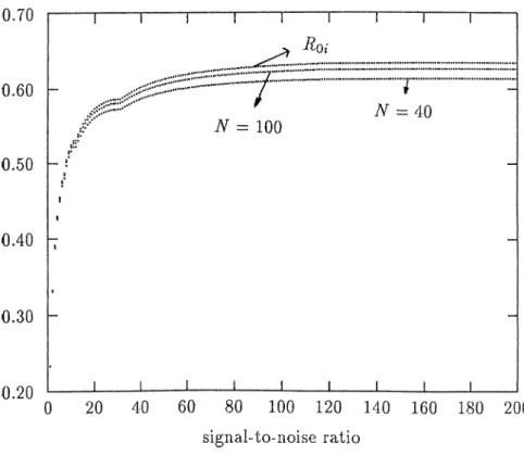
in Figures 2.3 to 2.42. In each case Rqí and iio/c with N = 40,100 are plotted. In the

case of no dark current (Aq = 0) similarly Rq versus A A curves for the ensembles of

independent-letters and fixed-composition codes are given in Figures 2.43 to 2.52.

Based on these figures our first observation is that one can get considerable im provements in the cutoff rate with fixed-composition codes. These improvements are listed in Tables 2.1 to 2.5. The improvement percentage is calculated by using Rqjc and

Rqí values (from the saturated region) for a fixed N and p as follows

a = - ^0» X 100

Rqx

We can achieve more than 80% improvement in cutoff rate for small values of p if fixed-

composition codes are used. This improvement decreases in low noise case as p increases, and for values of p close to 0.50, Rqí becomes greater than R o fc - The reason is that the independent-letters ensemble has more codewords than the fixed-composition ensemble, and in the low noise case (ideally in noiseless case) this is more dominating for obtaining higher cutoff rates.

(21)

CHAPTER 2. Ro ANALYSIS FOR FC AND IL ENSEMBLES 10

Another observation is the increase in cutoff rate when A A is increased at a fixed value the signal-to-noise ratio. This is because of the dependence of the cross-over probabilities of the DMC on AA as well as on the signal-to-noise ratio.

For given AA and SNR, increasing p results in an increase in the cutoff rate. This

is an expected result, because by increasing 2^ we increase the power for the corresponding message signal of the codeword.

The slope discontinuities in Figures 2.13 to 2.22 are due to the fact that as 7 in Equation 2.1 moves over integer values, the number of terms under summation in Equation 2.2 changes in a discrete manner.

Ill Ao = 0 case, there is only quantum noise and Rq increases obviously with AA, since we send more photons for one bit of information. For a specific value of A A , Rq increases with p similar to the case of Aq > 0.

After some value of N we expect that there will not be an improvement in cutoff

rate by increasing N, For AA = 2 case, cutoff rates for N = 40 and N = 100 are same

because saturation value of N is possibly achieved for smaller values than 40.

Consider an uncoded system in which there is no dark current, Aq = 0. Then, due

to Equation 2.2 (Z-channel of Figure 2.2) probability of error will be

P(E) = € =

where on the average we send | A A + ^0 = ^ photons/slot assuming 0 and 1 are equally likely. In order to achieve a probability of error, say, P{ E) = 10~® using this uncoded

system one should send approximately 10 photons/slot with rate, R = 1 bit/slot. Then,

efficiency will be 0.1 bits/photon. However, using coding, we can make P(E) arbitrar ily small by increasing constraint length and still send 10 photons/slot with a higher efficiency. For instance, using Figure 2.44 take A A = 3 photons/slot, since p = 0.10

we send on the average pAA = 0.3 photons/slot with rate Rq = 0.21 nats/slot = 0.3

bits/slot. This results in an efficieircy of 1 bit/photon which is ten times greater than that of uncoded system.

We can increase efficiency by increasing A and decreasing A where AA is held constant. Note that the rate of increase of Rq decreases as A A increases and at some point Rq saturates. But this causes an increase in the bandwidth. Large bandwidth is not a problem for optical systems but some practical problems may arise due to the hardware that should work with this system.

(22)

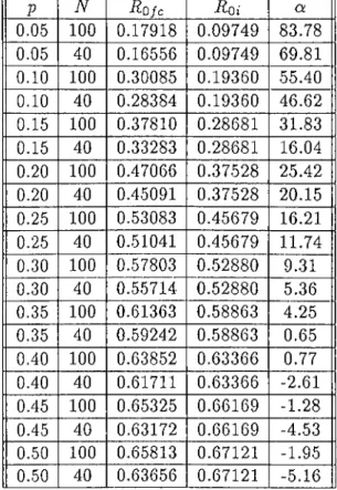
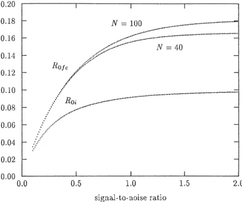
CHAPTER 2. Ro ANALYSIS FOR FC AND IL ENSEMBLES 11 P N Rofc Roi a 0.05 100 0.17918 0.09749 83.78 0.05 40 0.16556 0.09749 69.81 0.10 100 0.30085 0.19360 55.40 0.10 40 0.28384 0.19360 46.62 0.15 100 0.37810 0.28681 31.83 0.15 40 0.33283 0.28681 16.04 0.20 100 0.47066 0.37528 25.42 0.20 40 0.45091 0.37528 20.15 0.25 100 0.53083 0.45679 16.21 0.25 40 0.51041 0.45679 11.74 0.30 100 0.57803 0.52880 9.31 0.30 40 0.55714 0.52880 5.36 0.35 100 0.61363 0.58863 4.25 0.35 40 0.59242 0.58863 0.65 0.40 100 0.63852 0.63366 0.77 0.40 40 0.61711 0.63366 -2.61 0.45 100 0.65325 0.66169 -1.28 0.45 40 0.63172 0.66169 -4.53 0.50 100 0.65813 0.67121 -1.95 0.50 40 0.63656 0.67121 -5.16

(23)

signal-to-noise ratio

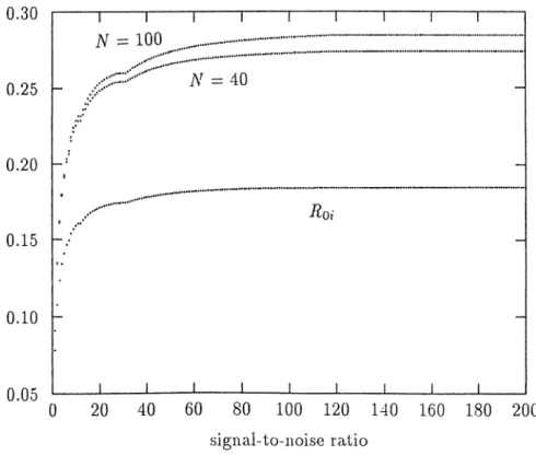
Figure 2.3; Rq/c for N — 100,40 and i2oi, 4lA = 50, p = 0.05

(24)

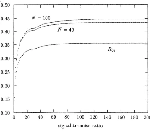
Figure 2.5: Rofc for H — 100,40 and Rq{, AA = 50, p = 0.15

(25)

sigiial-to-noise ratio

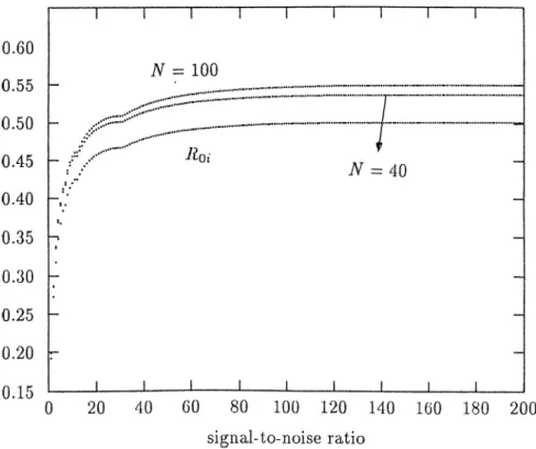
Figure 2.7: Rofc for N = 100,40 and i?oi, >1A = 50, j) — 0.25

(26)

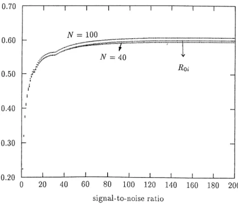
Figure 2.9: Rq/c for N = 100,40 and Roi, AA = 50, = 0.35

(27)

signal-to-uoise ratio

Figure 2.11: Rofc foï N = 100,40 and i2oi, = 50, p = 0.45

signal-to-iioise ratio

(28)

CHAPTER 2. Ro ANALYSIS FOR FC AND IL ENSEMBLES 17 P N R o f c Roi a 0.05 100 0.16915 0.09350 80.90 0.05 40 0.16019 0.09350 71.32 0.10 100 0.28473 0.18529 53.67 0.10 40 0.27420 0.18529 47.98 0.15 100 0.37482 0.27392 36.83 0.15 40 0.36349 0.27392 32.70 0.20 100 0.44688 0.35765 24.95 0.20 40 0.43504 0.35765 21.64 0.25 100 0.50451 0.43443 16.13 0.25 40 0.49230 0.43443 13.32 0.30 100 0.54976 0.50195 9.53 0.30 40 0.53728 0.50195 7.04 0.35 100 0.58392 0.55781 4.68 0.35 40 0.57125 0.55781 2.41 0.40 100 0.60781 0.59970 1.35 0.40 40 0.59501 0.59970 -0.78 0.45 100 0.62196 0.62572 -0.60 0.45 40 0.60908 0.62572 -2.66 0.50 100 0.62664 0.63454 -1.24 0.50 40 0.61374 0.63454 -3.28

(29)

Figure 2.13: Rqjc for N = 100,40 and Roi, AA = 10, p — 0.05

(30)

Figure 2.15: Rq/c for N = 100,40 and Roi, A A = 10, = 0.15

(31)

Figure 2.17: Rojc for N = 100,40 and R oi, A A = 10, p = 0.25

(32)

CHAPTER 2. Ro ANALYSIS FOR FC AND IL ENSEMBLES ₂₁

Figure 2.19: Rofc for N = 100,40 and Roi, AA = 10, p = 0.35

(33)

Figure 2.21: Rojc for — 100,40 and Rq{, /1A = 10, p = 0.45

(34)

CHAPTER 2. Ro ANALYSIS FOR FC AND IL ENSEMBLES 23 P N Rq fc Roi a 0.05 100 0.12109 0.07673 57.81 0.05 40 0.11975 0.07673 56.05 0.10 100 0.21138 0.15077 40.21 0.10 40 0.20921 0.15077 38.76 0.15 100 0.28350 0.22098 28.29 0.15 40 0.28075 0.22098 27.05 0.20 100 0.34192 0.28609 19.52 0.20 40 0.33876 0.28609 18.41 0.25 100 0.38900 0.34470 12.85 0.25 40 0.38553 0.34470 11.85 0.30 100 0.42616 0.39535 7.79 0.30 40 0.42246 0.39535 6.86 0.35 100 0.45431 0.43659 4.06 0.35 40 0.45044 0.43659 3.17 0.40 100 0.47405 0.46713 1.48 0.40 40 0.47006 0.46713 0.63 0.45 100 0.48575 0.48591 -0.03 0.45 40 0.48169 0.48591 -0.87 0.50 100 0.48963 0.49225 -0.53 0.50 40 0.48555 0.49225 -1.36

(35)

Figure 2.23: Rofc for N = 100,40 and Roi, AA = 5 , p - Q.05

(36)

Figure 2.25: Rofc for N = 100,40 and Roi, AA = 5, p = 0.15

(37)

Figure 2.27: Rofc for N = 100,40 and Roi, -4A = 5, p = 0.25

(38)

Figure 2.29: i?o/c for N = 100,40 and Roi, AA = 5, p = 0.35

(39)

Figure 2.31: Rofc foi' ^ = 100,40 and Rqi, AA = b, p = 0.45

1 r 0.55 0.50 0.45 h 0.40 0.35 - 0.30 - 0.25 H 0.20 0.15 h 0.10 0 Roi ..I··'·'“' J_______ L TV = 100 N = 40 J_______ L 20 40 60 80 100 120 140 160 180 200 sigiial-to-noisG ratio

(40)

CHAPTER 2. Ro ANALYSIS FOR FC AND IL ENSEMBLES 29 P N Rofc lioi a 0.05 100 0.07002 0.05291 32.32 0.05 40 0.06986 0.05291 32.02 0.10 100 0.12724 0.10276 23.82 0.10 40 0.12687 0.10276 23.46 0.15 100 0.17468 0.14890 17.31 0.15 40 0.17411 0.14890 16.93 0.20 100 0.21395 0.19069 12.20 0.20 40 0.21321 0.19069 11.81 0.25 100 0.24603 0.22746 8.16 0.25 40 0.24516 0.22746 7.78 0.30 100 0.27160 0.25859 5.03 0.30 40 0.27062 0.25859 4.65 0.35 100 0.29109 0.28349 2.68 0.35 40 0.29003 0.28349 2.31 0.40 100 0.30482 0.30166 1.05 0.40 40 0.30370 0.30166 0.68 0.45 100 0.31298 0.31273 0.08 0.45 40 0.31183 0.31273 -0.29 0.50 100 0.31569 0.31644 -0.24 0.50 40 0.31453 0.31644 -0.61

(41)

Figure 2.33: R o / c f o r N = 100,40 and Roi, AA = 2, p = 0.05

(42)

Figure 2.35: Rq/c for N = 100,40 and Roi, A A = 2, p = 0.15 0.22 0.18 0.14 -0.10 0.06 -0 . -0 2 1 r N = 100 N = 40 1--- T I ... ... ... / / Roi J_______ L J_ 0 20 40 60 80 100 120 140 160 180 200 signal-to-noise ratio

(43)

Figure 2.37: Rojc for N = 100,40 and AA = 2, j) = 0.25

(44)

Figure 2.39: Rq/c foi’ ^ = 100,40 and Roi, AA = 2, p = 0.35

0.30 0.25 -0.20 0.15 -0.10 0.05 1---Г N = 100 ,|H·“ 1111135·" N = 40 Roi / J_______ L 0 20 40 60 80 100 120 140 160 180 200 signal-to-noise ratio

(45)

Figure 2.41; Rq/c for N = 100,40 and Roi, AA = 2, p = 0.45

0..35 0.30 0.25 -0.20 0.15 - -· 0.10 -0.05 1 r iV = 40 "I r N = 100 ,.,..11···' ,„„•11·»»''*'·''"""]1^1 Roi ,1*'i·'*' I I I 0 20 40 60 80 100 120 140 160 180 200 signal-to-noise ratio

(46)

CHAPTER 2. Ro ANALYSIS FOR FC AND IL ENSEMBLES 35 P N Rofc Roi a 0.05 100 0.18137 0.09976 81.80 0.05 40 0.16648 0.09976 66.88 0.10 100 0.30482 0.19832 53.70 0.10 40 0.28557 0.19832 43.99 0.15 100 0.40073 0.29417 36.22 0.15 40 0.37901 0.29417 28.84 0.20 100 0.47730 0.38539 23.85 0.20 40 0.45395 0.38539 17.79 0.25 100 0.53845 0.46966 14.65 0.25 40 0.51395 0.46966 9.43 0.30 100 0.58641 0.54431 7.73 0.30 40 0.56109 0.54431 3.08 0.35 100 0.62260 0.60649 2.66 0.35 40 0.59669 0.60649 -1.62 0.40 100 0.64790 0.65340 -0.84 0.40 40 0.62160 0.65340 -4.87 0.45 100 0.66287 0.68264 -2.90 0.45 40 0.63635 0.68264 -6.78 0.50 100 0.66783 0.69257 -3.57 0.50 40 0.64123 0.69257 -7.41

(47)

:KAPTER 2. /¿0 ANALYSTS FOR FC AND IL ENSEMBLES 36

Figure 2.43: Rofc for N = 100,40 and Roi, Aq = 0, p = 0.05

(48)

C HA PT E R 2. R,, ANALYSIS FOR FC AND IL ENSEMBLES

Figure 2.45: i?o/c for N = 100,40 and i?ot, Aq = 0, p = 0.15

(49)

CHAPTER 2. R,y ANALYSTS FOR PC AND Tl ENSEMBLES 38

Figure 2.47: Rq/c for N — 100,40 and /¿оь Aq = 0, p = 0.25

(50)

CHAPTER 2. R,, ANALYSIS FOR FC AND IL ENSEMBLES 39

Figure 2.49: R o j c f o r N = 100,40 and i?oi, Aq = 0, p = 0.35

(51)

CHAPTER 2. /?,„ ANALYSIS FOR PC AND TL ENSEMBLES 40

Figure 2.51: i?o/c for N = 100,40 and Roi, Aq = 0, p = 0.45

(52)

CIIA PTFR 2. R,i ANALYSIS FOR FC A ND IT ENSEMBLES

2.4 Bounds for Cutoff Rates

41

An upper bound for Roi given by Equation 2.5 is

Roi = - ln(p^ + (1 - + 2p(l - p)z) < H{p) for 0 < z < 1

where

n (p ) = - p l n p - (1 - p )ln (l - p)

and z is given in Equation 2.6.

This bounding inequality is illustrated in Figure 2.53

(2.9)

(2.10)

Figure 2.53: 'T^(p) and Rq{, for z = 0 z = 0.9

We can also prove this fact as follows:

It is shown in Appendix that for any a,b > 0 and 0 < a- < 1

" < aa + (1 - a)b (2 .11) For p = 0 it is obvious that^ pP{l - pY ^ = p^ + (1 - pY- For 0 < p < \ substituting the values a — a — p, b = \ - a = l — p into Equation 2.11, we obtain

f { l - p Y ~ ' ^ <P^ T - i i - p f

(53)

Taking the natural logarithm of both sides of this final inequality we get

ln(pP(l - < ln(p^ + (1 - + (1 ~ pY + 2p(l - p)^) 0 < ^ < 1 which is nothing but Equation 2.9.

For RqJ} lower and upper bounds can be derived. In order to find an upper bound

for we can proceed by rewriting Equation 2.7

_r(^) e \ ^

N \ h \ *

K N - K _Ri K = pN

\

( N , ¿=0 \ \ P N (1 - p ) N \ ^2,· / (1 - p)N i > { ( l - p ) N - i y e > \ N N \ \ P N pN

E

i=0 pN \ fA - 2 p ,2 ( N \

For I j following inequalities hold [4, p.530]

1 e/VH(p) < ( iV \ ^ ^;vw(p)

y/m - [ p N J

-where 7i(p) is defined by Equation 2.10. Since N pN _ j_ N we can write e - < i > j:

(54)

CHAPTER 2. Ro ANALYSIS FOR EC AND IL ENSEMBLES 43

Using the well known binomial identity

§ ( ? ) ( %

we obtain

= , 1 + ---l - 2 p-z^ P

e > 1 + l - 2 p .-W(p)

Hence, an upper bound for Rq^I is found as follows:

4 / i < n p ) - pin f 1 +

V p

(2.12)

For obtaining lower bounds to Rq^} we can proceed as follows: Using the inequality

( l - p ) i V < ( ( l - p ) i V ) · e ^o/c < ^ \ i = 0 X N we can write / « M / V J ((1 - p)Nz'^y j < 1.06(1 + (1 - p)Nzye~^'^^P'> N > 40

This gives us the following lower bound on Rq^I

4 T c ^ '^(p) - P + (1 - P)Nz^) - ln(1.06) (2.13)

Another lower bound can be found [4, p.530] by noting that

( l - p ) N i < < 27t((1 - p)N — i) I ( 1 - P ) ^ Ai-v)Nn(H^) 2x(l — 2p)N Observing that ^ ^ P ^ ^ we obtain ■ l/N _p(N) '’1 ^ ('^ )(1 + ^2)P e 1— 1---!— - e«(p)

(55)

CHAPTER 2. Ro ANALYSIS FOR FC AND IL ENSEMBLES A4

So, an alternate lower bound for Rq^} is

Hip) - (1 - p)7i - p ln (l + < P R, (N) Ofc (2.14) Letting 5 1 = 'H{p) — p ln (l + (1 - p)Nz'^) - ln(1.06)) and 5 2 = H{i)) - (1 - p)!! j ~ as a result it can be written that

m a x (5 1 ,5 2 ) < Rq^^ < 'H{p) — pin Tl + — — z'^ P

For some cases the lower and upper bounds to Rqjci Roi versus p are given in Figures

(56)

CHAPTER 2. R,j ANALYSfS FOR FC AND JL ENSEMRIFS

P

Figure 2.54: Upper and Lower Bounds for Rojc and iiot> = 15, Aq = 0

(57)

r ' f l A F T E R 2. A N A L Y S I S F O R /•T' A Y E II, E Y S E M I U E S ■1fi

Figure 2.56: Upper and Lower Bounds for iio/c and Eoi, = 50, SNJl = 2

(58)

P

Figure 2.58: Upper and Lower Bounds for Rq/c and Roi, AA = 10, SNR 200

P

(59)

Chapter 3

CONCLUSION

As stated in Chapter 2, for the direct detection photon channel, fixed-composition codes exhibit better performance than independent-letters codes and we obtain a considerable improvement in cutoff rate. Also, the practical implementation is possible since Arikan [14] has recently proposed a method for constructing fixed-composition trellis codes with smallest possible degree which is independent of the blocklength.

In this work, we considered only ON -O FF‘ keying in which letters are chosen from a binary alphabet. It may be of interest to study multi-level signalling, li A =

{ A i, A2, A l} is an alphabet of size L with probability distribution {p i,P 2, then one should solve the problem of the optimization of Rq under the constraints:

= 1 5 ^^PiAi = constant which is a formidable problem.

Also, the sequential decoding of fixed-composition codes needs to be investigated further as pointed out in [14]. Namely, the problem stems from the memory introduced by the fixed-composition constraint; hence, optimum metrics for sequential decoding require excessive computation. However, trellis coding and sequential decoding part of the problem are left beyond the scope of this thesis work.

(60)

Appendix

P r o p o s itio n For any a,b > 0 and 0 < a < 1

< aa + (1 — a)b (3.1)

Proof

For 0 = 1 and a = 0 the above inequality holds with equality, so assume that 0 < o < 1. For t > 0 define = 1 — o + then,

= a — at°‘ ^ = o (1 = 0 => t = 1

For 0 < i < 1 < 0 and for t > 1 ^'(t) > 0. Therefore $ (i) has its minimum at

i = 1, hence Vi > 0 i ( i ) > $ (1 ) Vi > 0 1 - a + Q'i - i“ > 0 Substituting i = I we obtain Cl^ CL — < 1 - a + a j multiplying by 6 > 0 < aa + (1 - a)b 0 ^ 0 49

(61)

References

[1] Shannon, C.E., ‘A mathematical theory of communication,’ Bell Syst. Tech. J.,

vol.27, pp.379-423, July 1948.

[2] Wozencraft, J.M. and Kennedy, R.S., ‘Modulation and demodulation for probabilis tic coding,’ IEEE Trans. Inform. Theory, vol. IT-12, pp.291-297, July 1966.

[3] Viterbi, A.J., ‘Error bounds for convolutional codes and an asymptotically optimum decoding algorithm,’ IEEE Trans. Inform. Theory, vol. IT-13, pp.260-269, April

1967.

[4] Gallager, R.G., Information Theory and Reliable Communication. New York: John

Wiley & Sons, Inc., 1968.

[5] Snyder, D.L. and Rhodes, I.B., ‘ Some implications of the cutoff rate criterion for cod ed direct detection optical communication systems,’ IEEE Trans. Inform. Theory,

vol. IT-26, pp.327-338. May 1980.

[6] Davis, M.H., ‘ Capacity and cutoff rate for poisson-type channels.’ IEEE Tmns. Inform. Theory, vol. IT-26, pp.710-715, November 1980.

[7] Massey, J.L., ‘ Capacity,cutoff rate, and coding for a direct detection optical channel,’

IEEE Trans. Commun., vol. COM-29, p p .1615-1621, November 1981.

[8] McEliece, R.J., ‘Practical codes for photon communications,’ IEEE Trans. Inform. Theory, vol. IT-27, pp.393-397, July 1981.

[9] Bar-David, I. and Kaplan, G., ‘Information rates of photon-limited overlapping pulse position modulation channels,’ IEEE Trans. Inform. Theory, vol. IT-30, pp.455-

464, May 1984.

[10] Zwillinger, D., ‘ Differential PPM has a higher throughput than PPM for the band- limited and average-power limited optical channel,’ IEEE Trans. Inform. Theory,

vol. IT-34, pp.1269-1273, September 1988.

[11] Wyner, A.D., ‘ Capacity and error exponent for the direct detection photon chan nel,’ IEEE Trans. Inform. Theory, vol. IT-34, pp.1449-1471, November 1988.

(62)

51

[12] Georghiades, C.N., ‘ Some implications of TCM for optical direct detection chan nels,’ IEEE Trans. Commun., vol. COM-37, pp.481-487. May 1989.

[13] Forestieri, E., Gangopadhyay, R. and Prati, G., ‘Performance of convolutional codes in a direct detection optical PPM channel,’ IEEE Trans. Commun., vol. COM-37,

pp.1303-1317, December 1989.

[14] Arikan, E., ‘Trellis coding for high signal-to-noise ratio gaussian noise channels,’

Conference Record, IEEE Military Communication Conference, vol. 1, pp.196-199,