Channels Channel

Distributed Estimation with Channel Estimation

Error

over

Orthogonal Fading Channels

Habib

$enol

Department

of Computer Engineering

Kadir Has University

34083, Cibali, Istanbul, TURKEY

email. hsenol@,khas. edu. tr

Abstract-We study distributed estimation of a source cor-rupted by an additive Gaussian noise and observed by sensors which are connected to afusion center with unknown

orthog-onal (parallel) flat Rayleigh fading channels. The fading com-munication channels are estimated with training. Subsequently,

source estimation given the channel estimates and transmitted

sensorobservations is performed. We consider a setting where the estimated channels are fed-back to the sensors for optimal powerallocation which leads to a threshold behavior of sensors with bad channels being unused (inactive). We also show that

at least half of the total power should be used for training. Simulation results corroborate our analytical findings.

I. INTRODUCTION

Inatypical wirelesssensornetwork(WSN),alarge number ofsensors that each one observes the physical phenomenon represented by a parameter 0 are deployed randomly in a geological zone, and transmit their observations to the fusioncenter(FC) overthe wireless channels. FCwhich has less limitations in terms of processing and communication, whereassensorshave limitedprocessing and communication capability because of their limited battery power, receives transmissions from the sensors overthe wireless channels so as tocombine the receivedsignalstomake inferences onthe observedphenomenon.

Overthepastfewyears,research ondistributed estimation has been evolving veryrapidly [1]. Universal decentralized estimators of a source over additive noise have been con-sidered in [2], [3]. Much of the literature has focused in finite-rate transmissions ofquantizedsensorobservations [1]. The observations of the sensors can be delivered to the FC by analogordigital transmission methods. Amplify-and-forward isoneanalog option, whereas in digital transmission, observations are

quantized,

encoded and transmitted via

digital

modulation. The optimality of amplify and forward in several settings described in [4], [5]. In [5], amplify-and-forward over orthogonal parallel multiple access chan-nels(MAC) with perfect channel knowledge at the FC is

considered,

where

increasing

the number ofsensors is shown to

improve performance.

H. $enol is supported by The Scientific and Technological Research Council ofTurkey(TUBITAK) duringhisvisit as apost-doctoralresearcher

atArizona StateUniversity between Feb. 2007 andSept. 2007.

C.Tepedelenlioglu'sworkissupported byNSF CAREER grant No. CCR-0133841.

Cihan

Tepedelenlioglu

Department

of

Electrical Engineering

Arizona State University

85287

Tempe, AZ, USA

email.

cihan@,asu. edu

Unlike ourwork in [6] which considersno channel status information (CSI)atthesensorside with equal power alloca-tionamong sensors, hereweconsiderpower optimization in this estimated CSI setting, trading off feedback complexity withMSEperformance. Bydoing this,wefollow atwo-step proceduretofirst estimate the unknown fading channel coef-ficients withpilots, andusechannel estimates in constructing the estimator for the source signal with linear minimum mean square error(LMMSE) estimators.Wecharacterizethe effect of channel estimationerror onperformance for optimal power scheduling at the sensors, and imperfect estimated channels atthe FC.

We show that

increasing

the number of sensors will eventually lead to adegradation in performance for afixed total power. Hence, in the absence of channel information, deployingmore sensors might notnecessarily leadtobetter performance. We also characterize the penalty paid for estimating the channel tobe factor ofat least4 (6 dB).

II. SYSTEM MODELAND CHANNEL ESTIMATION

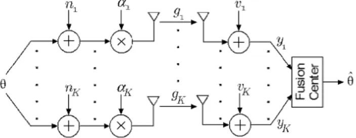
In our system model, as shown in Fig.1, we consider a wireless sensor network with K sensors whose

kth

sensor observes an unknown zero-mean complex random source signal 0 with variance

4o,

corrupted bya zero-meanadditive

complex

Gaussian noise nk

CA(O, or2 ).

Sincewe assume

the amplify-forward analog transmission scheme, the

kth

sensor amplifies its incoming analog signal 0 +nk by a factor ofak and transmits itonthe

kth

flatfading orthogonal channel to the fusioncenter

(FC).

In

Fig.

1,

gk

CAf(O,

or

2)

and Vk C-

(CO,

or)

are the flat

fading

channel

gain

and the channel noise of the

kth

channel path, respectively. The amplification factor ak varies with respect to the CSI

a, V

61 111

~~~~~~~~~~~~~o (D

+

YK

available at the sensor side. The kth received signal at the FC is given as

Yk =gkak

(O+nk)

+vk ,k= 1,.. .,K (1)

Wewill consider this receive model to estimate the source signal 0. Our two-step strategy, as illustrated in Fig.2, is first to estimate parallel channels, and then estimate the source signal given the channel estimates. We will use a LMMSE approach [7] for both steps. In the first phase, the sensors send training symbols of total power Ptrn to estimate the parallel channels

{gk

I}

K . In the second phase the sensors transmit their amplified data, which bear information about 0, with the optimally shared powers

{pk}K

1 among the

sensorswith respect to CSI. Note that the total power in the two phases add toPt0t. The fusion center uses the received signal in the second phase and the channel estimates from the first phase to estimate the source signal 0. To estimate

Fig.2. TrainingandData TransmissionPhases

the parallel fading channels

{gk},

1 in the training phase,

we considerpilot-based channel estimation as illustrated in Fig.3, where each sensor sends a pilot symbol to the FC

over its own fading channel. The receive model for apilot

s transmitted overthe kth channel is

Xk =gkS+vk (2)

where Xk is the received signal over kth channel and vk is

zero-mean additive complex Gaussian channel

noise,

nv

CA/(O, oa2).

Since the total transmittedtrainingpowerisPtrn,

wehave Ptrn =K s2. According to our observation model

III. SOURCE ESTIMATION AND POWERALLOCATION

After estimation of the unknown fading channels in the first phase, in the second phase, we estimate the source signal 0 by choosing an LMMSE type source estimator given the channel estimates

{gMk}k=

in (3), and the received signal

Yi,

. . ,YK in (1). In other words, we obtain the

sourceestimator 0 in the presence of channel estimation error (CEE). The resulting MSE of source estimator will be our figure of merit. Exploiting the orthogonality principle of the LMMSE estimator, it is possible to give the minimum MSE in the presence of CEE as follows [8]

D=ao

I K1( kU

(9

2

+2)pk+2)

(

rk

(gJ2

62)

+

(62

)Pk +

(J2J

with the following definitions:

Here,

we express

te

cnannei

(4)

and

Ptrn

K

IS12

as

(5)

estimator variance o using

(6) Substituting (6) into (5), it is straightforward to verify that (5)is a convex function of

{Ptrn,

P1I

. PK}by taking the second derivative. For the purposes of optimization of the MSE in (5) with respect to {Ptrn

PI,

...

PKI},

it suffices

towork with

K Pmk2( _ 2)Pk

(k

k

62)

+

((2

)

pk

+72 (7)

1

Fig. 3. Channel EstimationScheme forOrthogonal MAC Channels

in (2), the linear minimum mean square error (LMMSE)

estimate g, of the channel g, is given as follows [7]

A_Et97g,X7C}

[

gkX*

I

gk E{9,1}[gkx2] E f, [Xkl21 a2* 9 , U2 + U2 S12 v 9 (3)

where (.)* denotes the complex conjugate and the channel estimation errorvariance 62 is givenas

62

- + s

aT2

a2

U2+

(72

IS2

av 9

(4)

The above function is ageneral form of the convex objective functions considered in thesequel.Wewill work withspecial

cases of(7)toobtain MSE expressionsboth in the presence and absence of CEE. Beforeweoptimizethetraining power,

wewill briefly review theperfect CSI case.

A. Perfect CSI Case

With perfect CSI both at the FC and sensor side, the variance of the CEE is zero, 62 = 0, and the normalized

estimated channel powers are equaltothe normalized chan-nel powers

7k

=

'lk

Vk. By substituting62 =0and

7k

=

'7k

in (7),the optimization problemfor the perfect CSI case is obtained as follows a k Pk min

-vE

'T P1, ,PK k=1'7kPk+ I K s.t.

Pk<

Ptot

k=1 Pk>O , k=1,2, ,K, (8) Variance ofgk g? =(72 _62 Observation SNR

2Y:

2

Total training power Ptrn:= K s

12

k±h

sensordata transmissionpower

Pk

2

Channel SNR : U29 2

k±h

estimated channel power : k (5 2 a2) (^+1)

9 2k

k±h

channelpower

'lk

o7

(y±l)

g

s

62

=

(Ka2

)

/(K

+

(Pt,,).

where the optimization is with respect to the transmitpowers atthesensors. This problem is consideredin [5] for the best linear unbiased estimator (BLUE). Adapting to the LMMSE

case,the optimumpowers are given by

(6)

A2Ptrn

0

A2

(7)

> 0

Ptrn

(8)

> 0 1 k- EI MEA ( ~ + r4 '712) k (Per) (9)

where A := TmlTm > T(per)} is the set of active sensors

whose data transmission powers arepositive (i.e. Pk >0 or equivalently Tlk > T(Per)), and the threshold value T(per) iS given by

T(per) (10)

The sensors whose channel powers are below the threshold level are turned off in the data transmission phase.

B. EstimatedCSI Case

Inthe estimated CSI case, we assume that parallel chan-nels

{gk

k= are estimated at the FC and the channel estimates are fed back from the FC to sensors in order to

perform the optimal data power allocation strategy. So, after training, the remaining power

Ptot

-Ptrn is optimally shared among the sensors. Therefore, substituting (6) into (7) we get the

objective

function of the following convex

optimization problem K min S

Tlk71

Ptrn Pk

Pt,n,Pi,

,PK k=1 'k

kPtrnPk

+

K(Pk

+¢Ptrn+ K K s.t. Ptrn+Pk < Ptot k=1

Ptrn

>0 Pk>0, k= 1,2,

,K.

(11)

Now wesolvetheproblem in (11). The Lagrangian function is given by K

='k

_EPtrnPk k7=1k ¢PtrnPk +

K(Pk

+¢Ptrn+ K K K

-AI(Ptot-Pt-

Pk)-A2Ptrn-

5P§kPk

k=1 k=1

and the following Karush-Kuhn-Tucker conditions are de-rived from theLagrangian function [9]:

K

-y

Kk

(

(Pk +1) Pk (1) A A=1

(7k

¢PtrnPk +

K(Pk

+¢Ptrn +

K)2

Al

ttky-1k(

(¢Ptrn

+

K)

Ptrn

('k

(PtrnPk

+

K(Pk

+

(Ptrn

+K)2

(2)

0 Vk, K

(3)

(4)

K

(5)

A

1(Ptot-Ptrn -Pk)

°0

A1

> ,

Ptrn+SPk<

Ptot

k=l k=l

(9)

(10)

(I

1)

PkPk

= 0

Vk

Pk>_0

Vk

Pk

>0V

k.

(12)

where (12.1) and (12.2) are obtained by

8LI8Ptrn

0 and

8LI8Pk

= 0,respectively. We will assume0< Ptrn <

Ptot

which means A2 = 0as seenfrom the condition (12.6). From

conditions (12.9) and (12.11) active sensors with Pk > U

have corresponding Lagrange multipliers ,k = 0. We now

want to determine how much optimum data transmission powerhas to be allocated for each active sensor. The condi-tion (12.2) canbe rewritten for active sensors (i.e., Pk > 0

and Ilk =0) as

Pk+

1l+p

( A

1P,

Pk >0 (13)

Using (13), it follows that for active sensors (Pk > 0) we

have

r1k

> A

(I

+ K ). This means that

r1k

ifexceeds

the following threshold

T(est) = (1+ ,j

K)

(14)

the kth sensor will be activated in the data transmission phase.Intheequations (13) and (14), the Lagrange multiplier A1 still needs to be determined. Letthe activesensor setbe defined as B :=

I1

'7 > T} for the estimated CSI case.

Recalling E Pe =

Ptt-

Ptrn, we sum both sides of (13) CEB

1+(P>t,K nl_ / A/1' 1+(PItl

K)

) 1

Ptot

Ptrn+5

+P1

K:

+ K

(15)

£EB'7 Ptrn 1EB Ptr

Solving for A1 in (15) and substituting into (13) and (14) the optimal data power

Pk*

and the threshold level T(est) are

obtained as '7k k- E

P4n

'7k+ K pEB Ptrn 1+ K

'7k

+ K Ptrn and

Ptot

Ptrn

+ 1+ KK J V

1,k

>T(est) ₍₁₆₎ (

(+

K)

~2

Tr(est) =ID

Ptrn+

(1

(1+)f

E L

1P1

(17)

\Ptot

-BPtrn

+

(I

+ K ) I

respectively. As seen from (16) and (17), the optimum data transmission power per sensor and the threshold depend on

the training powerPtrn. We now want tofind the optimum training power

Ptrn.

Substituting (12.2) into (12.1),we get the following equation,

trn2 trn

and note that the total optimal training power

Pt*,,

depends onthe power of active sensors,

Pf

.Equations (16) and (18) show that

Pk*

and

Pt*rn

depend on each other and the channel realizations. Since the total training power Ptrn must be selected without knowing the channel realizations, we would like to bound it with a value that is not channel dependent. Toward this goal, we use Cauchy-Schwartz inequality,

I: 2 > I

fEB

(E) > ()E 2

where

IB

is the cardinality of the set of active sensors. Substituting the above lower bound into (18), and using

Z Pe =

Ptt-Pt*,P,

onthe

right

hand

side,

we obtain the

£EB

following lower bound on the optimal training power

Pt*,,:

Ptot

Ptrn

>-

2 (20)

which establishes that the total training power should be chosenatleast half of the total power.

C. Comparison of Perfectand Estimated CSI Cases

In subsection, we want to find the relationship between total power of the perfect and estimated CSI cases,

P1(Pter)

and

P(jes),

that wouldensurethat the MSE in thetwo cases

would have the same distribution, for a finite number of

sensors and large total power. More concretely, our goal is to determine the ratio of the total powers of the perfect andimperfectCSIcasesfor identical distributed MSEs while total power goestoinfinity. Since

Pt*,,

>

Ptot/2

from(20), when

Ptot

-) oc, the optimum training power

Pt*n

-' °o which means that channel estimation errorvariance goes to zero

(62

-)

0)

as seen from (6). Eventually, the estimated channel powers approach tothe true channel powers r1k -' Tlk Vk since channel estimates approach to true channels -k gk Vk.

Additionally,

with

large

total powers, all the

sensors become active, for both perfect and estimated CSI

cases because threshold levels in (10) and (17) go to zero asthe total powers goesto infinity. Under these conditions,

we wish to make the objective functions for perfect and estimated CSI cases in (8) and (11) equal which ensures

that the resulting solutions will be the same. The objective functions in(8) and(11) are equal ifand only if

K_{K +}

_(i+

_Jr)K I

_est)

Ptrn (Ptrn pk(et

wherePk(P ) andPk(st) arethe powers

sensor in the perfect and imperfect chz

K

tively. Keeping in mind E

Pk(Per)

k=l

both sides of(21) by

Pk

(Per) and summir (21) as

K Pk

k=1Pk(

Multiplying both sides of (22) byP(est)

p(Pter)

and inverting both sides of the equation, we have the following expression for the power ratio P(Per) p(est)

tot

t;ot

p(per) pp(est) (ot K p(per) 1

tot

tot)

petot _{+ +} Ptrn

j(2p(3t

tot (23)

p(estot Ptrn WK

(pto

/ p(t),

Recalling

P(Per)

-) 00_tottogether with P(est)_~~~~~~~tot-,oC, from (9)

and (16) we obtain the limit of the

kth

summation term in (23) as follows

Pk(per)

p(per)

lim tot

p(est)

Pk(est) tot --I'Ip(est)

tot

1

1 urn

~~p,-t)

p(est)--,I tote tot -0

1

1-r'

(24)

where weused

r1k

-

Tlk,

andr is definedasthe asymptotic

ratio between the training and the total powers of the estimated CSI case as follows

r,=

l{im

Ptrn

(est)

--,Ip(est)

tot tot

(25) For agiven r, substituting (24) and (25) into (23) and taking the limit, the asymptotic power penalty ratio between the total powers ofperfect and estimated CSI cases that make the MSEs identical is obtained as

p(per) 1 1 1

p(est)

Pt(ot)

e

r

1

r)

(

)

(26)

tot

is -cr00 tot

It is clear from

(26)

that the maximum ratio is obtained as p(per)

lim tot

p(est) p(est) Ptot --,I tot

1

4 (27)

when r=

1/2

(50% training power). We can thus conclude

that for largetotal transmit powers, the penalty paid for not

knowingthe channel is 6 dB, which is achieved when

Ptrn

is half the total power.

IV. NUMERICALRESULTS

In Fig.4, we illustrate that there is an optimum number

1 (21) of sensors that minimize the MSE. We also observe that

Pk

(per) the number of sensors that minimize the MSE increases as

the total power

Pt3t

increases for the estimated CSI case

allocatedtothekth with a

60%c

training power ratio. Fig.4 confirms that the annel cases, respec- MSE performance in the estimated CSI case is exhibiting

p(per) multiplying adegradation beyond an optimumnumber ofsensors. In Fig.5, the power penalty ratios on the horizontal axis ng,we canreexpress can be read off when the average MSEs are equal (the y-axis is one), and the power penalty ratio

P(Per)

p(etst)

is seen to be about 0.24 for the MSE

performances

of

perfect

and

_=

1

(22)

imperfect

channelcasestobe

equal

withr

=

PtrnlP(es8t)

est)

60%c

when the sensor powers are optimized.

p(per)

I I

tot + +

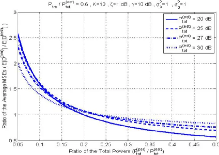
The curves in Fig.6 are plotted for various training power ratios for the estmated CSI case. In this figure, we observe that the asymptotic ratios of total powers are

roughly

Pt(Pter)

Pt(et)

=

0.25,

0.24,

0.21 and 0.16 forr

Ptrnt

(ost

0.5,

0.6,

0.7 and

0.8,

respectively,

which is predicted by (26).

V. CONCLUSIONS

In this work, we study the effect of fading channel estimationerror onthe performance of distributedestimators ofasource0.Atwo-phaseapproach was employed where in the first phase, the fading coefficients are estimated, and in the second phase, these estimatesand the received signal are usedto estimate the source 0. The optimum training power in this setting was shown to be greater than half the total power. In assessing the loss in total power due to channel estimationinthis optimizedsensor powersetting, we used an asymptotic analysis wherethe total transmit power was large. It wasfound that the power penalty ratio between perfect and imperfect CSI cases was about 6 dB.

60%ofPtot =1dB, 10 dB 2=1 2=1

Fig. 4. Average MSE vs.number of sensors for the estimated CSI case

pt/p(t)=0.6,K=10, -!15 D 2.5 Li] -!7 L1] 2 cn LU lo 1. =1dB, -10dB, 2=1, 2=1 2 D 1.8 j_ -w5 1.6 cn a) X 1.2 8I 0 0.8 p(t) 30dB, K=10, 1=ldB, 10 dB 62=1 62=1 ot.0 9-Ptr 05 ... pte )= ~p(t 065 /pt(est) 07 p t 086 0.05 0.1 0.15 0.2 0.25 0.3 0.35 0.4 Ratio of the Total Powers rI t))

0.45 0.5

Fig. 6. Ratio of theaverage MSEs vs. ratio of the total powers for different r=Pt,n

Ptett)

ratios

REFERENCES

[1] Jin-Jun Xiao, A. Ribeiro, Zhi-Quan Luo, andG.B. Giannakis, "Dis-tributedcompression-estimationusing wireless sensor networks," IEEE SignalProcessing Magazine,vol. 23, no. 4, pp. 27-41, July 2006. [2] Z.-Q. Luo, "Universal decentralized estimation in a bandwidth

con-strained sensor network," IEEE Transactions on Information Theory, vol. 51, no. 6, pp. 2210-2219, June 2005.

[3] Jin-Jun Xiao, Shuguang Cui, Zhi-Quan Luo, and A.J. Goldsmith, "Power scheduling of universal decentralized estimation in sensor networks," IEEE Transactions on Signal Processing, vol. 54, no. 2, pp. 413-422, February 2006.

[4] M. Gastpar, B. Rimoldi, and M. Vetterli, "To code or not to code: Lossysource-channel communication revisited," IEEE Transaction on Information Theory, vol. 49, pp. 1147-1158, May 2003.

[5] S. Cui, J.-J. Xiao, A. J. Goldsmith, Z.-Q. Luo, and H. V. Poor, "Estimation diversity and energy efficiency in distributed sensing," IEEETransactions onSignal Processing, vol. 55, no. 9, pp. 4683-4695, September2007.

[6] H. Senol and C.Tepedelenlioglu, "Distributed estimation over parallel fadingchannels with channel estimationerrors," in ICASSP 2008, Las Vegas,NV,(under review).

[7] S. M.Kay, Fundamentals ofStatisticalSignal Processing: Estimation Theory,PrenticeHall, New Jersey, 1993.

[8] H.Senol and C.Tepedelenlioglu,"Distributed estimation over unknown parallel fading channels," IEEE Transactions on Signal Processing, (under review).

[9] S. Boyd and L. Vanderberghe, Convex Optimization, Cambridge University Press,Cambridge,UK,2003.

0.05 0.1 0.15 0.2 0.25 0.3 0.35 0.4 0.45 0.5 Ratio of the Total Powers prI t))

Fig. 5. Ratioof the average MSEs vs. ratio of the total powers

_p(etst)=20 dB p(est)=25 dB ..I.p.(est)=27 dB """'PIest)=30 dB o1 0.5'