Anomaly detection with sparse unmixing and gaussian mixture modeling of hyperspectral images

ANOMALY DETECTION WITH SPARSE

UNMIXING AND GAUSSIAN MIXTURE

MODELING OF HYPERSPECTRAL IMAGES

a thesis submitted to

the graduate school of engineering and science

of bilkent university

in partial fulfillment of the requirements for

the degree of

master of science

in

computer engineering

By

Acar Erdin¸c

July, 2015

ANOMALY DETECTION WITH SPARSE UNMIXING AND GAUS-SIAN MIXTURE MODELING OF HYPERSPECTRAL IMAGES By Acar Erdin¸c

July, 2015

We certify that we have read this thesis and that in our opinion it is fully adequate, in scope and in quality, as a thesis for the degree of Master of Science.

Assoc. Prof. Dr. Selim Aksoy(Advisor)

Assoc. Prof. Dr. Hakan Ferhatosmano˘glu

Assist. Prof. Dr. Seniha Esen Y¨uksel

Approved for the Graduate School of Engineering and Science:

Prof. Dr. Levent Onural Director of the Graduate School

ABSTRACT

ANOMALY DETECTION WITH SPARSE UNMIXING

AND GAUSSIAN MIXTURE MODELING OF

HYPERSPECTRAL IMAGES

Acar Erdin¸c

M.S. in Computer Engineering Advisor: Assoc. Prof. Dr. Selim Aksoy

July, 2015

One of the main applications of hyperspectral image analysis is anomaly detec-tion where the problem of interest is the detecdetec-tion of small rare objects that stand out from their surroundings. A common approach to anomaly detection is to first model the background scene and then to use a detector that quantifies the difference of a particular pixel from this background. However, identifying the dominant background components and modeling them is a challenging task. We propose an anomaly detection framework that uses Gaussian mixture models for characterizing the scene background in hyperspectral images. First, the full spectrum is divided into several contiguous band groups for dimensionality reduc-tion as well as for exploiting the peculiarities of different parts of the spectrum. Then, sparse spectral unmixing is performed for each band group for identifying significant endmembers in the scene. Three methods for identifying the dominant background groups such as thresholding, hierarchical clustering and biclustering are used in the endmember abundance space to retrieve the sets of pixel groups that represent dominant background components. Next, these pixel groups are used for initializing individual Gaussian mixture models that are estimated sep-arately for each spectral band group. The proposed method enables automatic identification of the number of mixture components and effective initialization of the estimation procedure for the mixture model. Finally, the Gaussian mix-ture models for all groups are statistically fused for obtaining the final anomaly map for the scene. Comparative experiments showed that the proposed methods performed better than two other density-based anomaly detectors, especially for small false positive rates, on an airborne hyperspectral data set.

Keywords: Anomaly detection, spectral unmixing, Gaussian mixture model, hi-erarchical clustering, biclustering, hyperspectral imaging.

¨

OZET

H˙IPERSPEKTRAL G ¨

OR ¨

UNT ¨

ULERDE SEYREK

SPEKTRAL AYRIS

¸TIRMA VE GAUSS KARIS

¸IM

MODEL˙I ˙ILE ANOMAL˙I TESP˙IT˙I

Acar Erdin¸c

Bilgisayar M¨uhendisli˘gi, Y¨uksek Lisans Tez Danı¸smanı: Assoc. Prof. Dr. Selim Aksoy

Temmuz, 2015

Anomali tespiti, hiperspektral g¨or¨unt¨u analizindeki ana uygulamalardan biridir. Anomali tespitindeki problem, g¨or¨unt¨ude seyrek olarak bulunan, ¸cevresine g¨ore farklılık g¨osteren k¨u¸c¨uk nesnelerin tespitidir. Yaygın yakla¸sımlardan biri g¨or¨unt¨u arka planının modellenmesi ve sınanan pikselin bu modele olan farklılı˘gına g¨ore sınıflandırılmasıdır. Ancak, karma¸sık arka planların modellenmesi kolay de˘gildir. Bu kapsamda, Gauss karı¸sım modeli tabanlı bir anomali tespiti y¨ontemi ¨

onerilmektedir. ¨Oncelikle g¨or¨unt¨u belirli sayıda spektral gruplara ayrılmaktadır. Ardından seyrek spektral ayrı¸stırma b¨ut¨un spektral grouplarda uygulanmak-tadır. Sonrasında, elde edilen son eleman bolluk de˘gerleri kullanılarak, e¸sikleme tabanlı, sıra d¨uzenli tabanlı, ve ¸cift y¨onl¨u ¨obekleme tabanlı olmak ¨uzere ¨u¸c farklı y¨ontem ile baskın arka plan grupları tespit edilmektedir. Ardından, belir-lenen arka plan gruplarını temsil eden pikseller ba¸slangı¸c de˘gerlerinin hesaplan-masında kullanılmak ¨uzere, her bir spektral grup i¸cin bir Gauss karı¸sım modeli ¨

o˘grenilmektedir. ¨Onerilen y¨ontem karı¸sım modeli i¸cin bile¸sen sayısının otomatik belirlenmesine ve kestirim s¨urecinin etkili ba¸slatılmasına olanak sa˘glamaktadir. Son olarak, ¨o˘grenilen Gauss karı¸sım modelleri istatistiksel olarak birle¸stirilerek sonu¸c anomali haritası elde edilmektedir. Deneysel veriler g¨ostermektedir ki ¨

onerilen y¨ontemler, ¨ozellikle d¨u¸s¨uk yanlı¸s alarm de˘gerleri i¸cin, di˘ger y¨ontemlere g¨ore daha y¨uksek performans sa˘glamaktadır.

Anahtar s¨ozc¨ukler : Anomali tespiti, spektral ayrı¸stırma, Gauss karı¸sım modeli, sıra d¨uzenli k¨umeleme, ¸cift y¨onl¨u ¨obekleme, hiperspektral g¨or¨unt¨uleme.

Acknowledgement

Firstly, I would like to thank Assoc. Prof. Dr. Selim Aksoy for giving me the opportunity to work with him and learn from him, and his guidance throughout my degree.

Special thanks to Assoc. Prof. Dr. Hakan Ferhatosmano˘glu and Assist. Prof. Dr. Seniha Esen Y¨uksel for kindly accepting to be in my committee. I owe them my appreciation for their support and helpful suggestions.

I want to thank Ecem Sıla Karslı for her friendship and love, and for accom-paninying my journey.

Finally, I would like to deeply thank my beloved family for always being there for me and their never-ending trust in my success.

This thesis is partially supported by Havelsan, Inc. I also would like to thank Havelsan, Inc. for collecting and preparing the data set.

Contents

3.3 Dominant Background Groups . . . 17

3.3.1 Thresholding . . . 19

3.3.2 Hierarchical Clustering . . . 21

3.3.3 BiClustering . . . 24

3.4 Probabilistic Background Modeling . . . 28

CONTENTS vii

3.4.2 Expectation Maximization (EM) . . . 29

3.5 Partition Combination . . . 30

4 Experiments 32 4.1 Dataset . . . 32

4.2 Baseline Methods . . . 33

4.3 Results . . . 35

4.3.1 Baseline Methods Results . . . 36

4.3.2 Havelsan Spectral Library Results . . . 40

4.3.3 USGS Spectral Library Results . . . 46

4.3.4 Discussion . . . 52

List of Figures

1.1 Hyperspectral imaging concept. Taken from Bioucas-Dias et al. [1]. 2

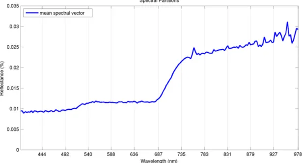
3.1 Spectral partitions are illustrated with the vertical grid lines for the mean spectral vector of the hyperspectral image. . . 13

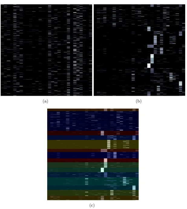
3.2 Hierarchical clustering examples from our experiments on the abundance feature space. (a) Raw abundance matrix. (b) Rear-ranged abundance matrix. (c) RearRear-ranged hierarchical clustering result. . . 22

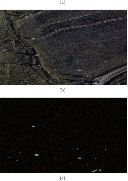
3.3 Hierarchical clustering examples from our experiments on the im-age feature space. (a) Mean vectors of the clusters. (b) Pixels associated with the 3 clusters that have the highest coverage are overlayed on the RGB image. (c) Pixels associated with the 3 clus-ters that have the highest coverage are overlayed on the ground truth image. . . 23

3.4 BiClustering example of rearranged biclusters that reveal a checkerboard structure. Taken from the official Scikit-Learn web page [2]. . . 25

3.5 BiClustering examples from our experiments on the abundance fea-ture space. (a) Raw abundance matrix. (b) Rearranged abundance matrix. (c) Rearranged biclustering result. . . 26

LIST OF FIGURES ix

3.6 Biclustering examples from our experiments on the image feature space. (a) Mean vectors of the clusters. (b) Pixels associated with the 3 clusters that have the highest coverage are overlayed on the RGB image. (c) Pixels associated with the 3 clusters that have the highest coverage are overlayed on the ground truth image. . . 27

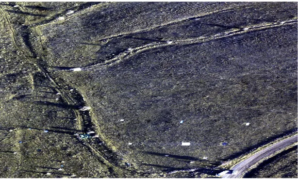
4.1 RGB image. . . 33

4.2 Binary mask of 19 small objects. . . 34

4.3 Anomaly detection results for the RX detector before post-processing. (a) Log-probability anomaly map. (b) Binary detec-tion map. . . 36

4.4 Anomaly detection results for the RX detector after post-processing. (a) Log-probability anomaly map. (b) Binary detec-tion map. . . 37

4.5 Anomaly detection results for the RX-GMM detector before post-processing. (a) Log-probability anomaly map. (b) Binary detec-tion map. . . 38

4.6 Anomaly detection results for the RX-GMM detector after post-processing. (a) Log-probability anomaly map. (b) Binary detec-tion map. . . 39

4.7 Anomaly detection results for Havelsan Spectral Library and the thresholding based method before post-processing. (a) Log-probability anomaly map. (b) Binary detection map. . . 40

4.8 Anomaly detection results for Havelsan Spectral Library and the thresholding based method after post-processing. (a) Log-probability anomaly map. (b) Binary detection map. . . 41

LIST OF FIGURES x

4.9 Anomaly detection results for Havelsan Spectral Library and the hierarchical clustering based method before post-processing. (a) Log-probability anomaly map. (b) Binary detection map. . . 42

4.10 Anomaly detection results for Havelsan Spectral Library and the hierarchical clustering based method after post-processing. (a) Log-probability anomaly map. (b) Binary detection map. . . 43

4.11 Anomaly detection results for Havelsan Spectral Library and the biclustering based method before post-processing. (a) Log-probability anomaly map. (b) Binary detection map. . . 44

4.12 Anomaly detection results for Havelsan Spectral Library and the biclustering based method after post-processing. (a) Log-probability anomaly map. (b) Binary detection map. . . 45

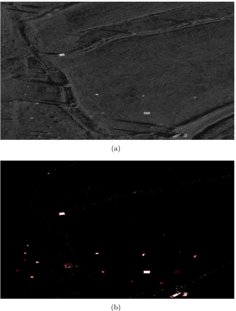
4.13 Anomaly detection results for the USGS Spectral Library and the thresholding based method before post-processing. (a) Log-probability anomaly map. (b) Binary detection map. . . 46

4.14 Anomaly detection results for the USGS Spectral Library and the thresholding based method after post-processing. (a) Log-probability anomaly map. (b) Binary detection map. . . 47

4.15 Anomaly detection results for the USGS Spectral Library and the hierarchical clustering based method before post-processing. (a) Log-probability anomaly map. (b) Binary detection map. . . 48

4.16 Anomaly detection results for the USGS Spectral Library and the hierarchical clustering based method after post-processing. (a) Log-probability anomaly map. (b) Binary detection map. . . 49

4.17 Anomaly detection results for the USGS Spectral Library and the biclustering based method before post-processing. (a) Log-probability anomaly map. (b) Binary detection map. . . 50

LIST OF FIGURES xi

4.18 Anomaly detection results for the USGS Spectral Library and the biclustering based method after post-processing. (a) Log-probability anomaly map. (b) Binary detection map. . . 51

4.19 ROC curves for the proposed methods that are using the Havel-san Spectral Library and the baseline methods. (a) Before post-processing. (b) After post-post-processing. . . 53

4.20 ROC curves for the proposed methods that are using the USGS Spectral Library and the baseline methods. (a) Before post-processing. (b) After post-post-processing. . . 54

List of Tables

4.1 Ground truth objects in the scene. . . 34

4.2 AUC values of the proposed methods that are using the Havelsan Spectral Library and the baseline methods. . . 52

4.3 AUC values of the proposed methods that are using the USGS Spectral Library and the baseline methods. . . 52

Chapter 1

Introduction

Recent improvements in hyperspectral imaging technologies enabled the devel-opment of both high spectral and high spatial resolution instruments that are used in Earth observation and remote sensing [1]. The cameras used for the data acquisition of such imagery can operate in a wide spectrum of wavelengths. The most important of them all are those operating in the visible, near-infrared, and shortwave infrared spectrum, ranging from 0.3 µm to 2.5 µm [3]. High spec-tral resolution in hyperspecspec-tral images provides the capability to discriminate the physical characteristics of different materials and enables their identification in remotely sensed scenes. In Figure 1.1, the hyperspectral imaging concept is visualized. Each plane corresponds to all of the pixels’ radiance acquired over a spectral band. Each pixel is a spectral vector that represents the radiance read-ings for all spectral bands in a location. The data cube is the entirety of the planes.

One of the most common applications of hyperspectral imaging is target detec-tion. Prior knowledge about the target of interest and its spectral characteristics allows us to operate on a single spectrum [4] or a subspace spectrum [5] that defines the target. In such a case, signature-based target detection methods are commonly used [6]. However, the target signatures are not always available. Be-cause of this unavailability, anomaly detection approaches are usually considered

Figure 1.1: Hyperspectral imaging concept. Taken from Bioucas-Dias et al. [1].

to be an alternative. The scenario where the problem of interest is the detec-tion of small rare objects or materials that have different spectral characteristics compared to their surroundings is called anomaly detection. Anomaly detection has been a popular problem in remote sensing where the common approach is to first model the image background and then to use a detector that quantifies the difference of a particular pixel from this background as the confidence of an anomaly existing at that pixel.

Numerous approaches for both background characterization and detector func-tions have been proposed in the literature [7]. For a hyperspectral image Y = (y₁, . . . , y_{N) ∈ R}L×N where y_{i ∈ R}L is the i’th pixel, N is the number of pixels and L is the number of spectral bands, the common approach for an anomaly detection scenario is to find a suitable background model p(y|θ) so that an approximation to the background probability p(background |y) can be made. In which case, the probability of a pixel being an anomaly becomes

and the decision criteria can be defined as assign y as    anomaly if p(anomaly|y) > τ background , otherwise, (1.2)

where τ is the detection threshold.

In this thesis, our focus is on the modeling of complex scenes that contain an unknown number of background materials in an anomaly detection scenario. The commonly used RX anomaly detector [8] and many of its various extensions do not necessarily perform well in complex scenes due to the heterogeneity of the image background and the limitations of the single multivariate Gaussian in modeling the multiple land cover classes existing in that background. A popular alternative has been to use a Gaussian mixture model (GMM) based on the assumption that the background consists of multiple classes each of which can be modeled using a separate Gaussian component in the mixture [9]. However, GMM-based back-ground modeling has two important issues: there is often no prior information regarding the number of components, and GMM estimation using all spectral bands may suffer from the curse of dimensionality due to increasing model com-plexity with increasing number of components. The former issue can be solved by an empirical search procedure when the number of different background ma-terials is unknown in an unsupervised setting. The latter issue often necessitates a dimensionality reduction step, such as principal components analysis (PCA), prior to GMM estimation. However, there is no unanimously accepted procedure regarding which principal components should be used. There is also the poten-tial problem that the resulting transformation that tries to maximize the data variance may not retain important discriminative information embedded in the original spectral bands.

In this thesis, we use a GMM-based background model for anomaly detection. First, we perform spectral partitioning to reduce the data dimensionality while preserving the original physical characteristics of the input data. After dividing the data into several groups of contiguous spectral bands, we perform spectral unmixing to identify the number of dominant endmembers and to automatically determine the number of components in the background model. To do so, we

propose three methods for identifying dominant background groups. The first method is named as thresholding as we apply a set of thresholds on the frac-tional abundance space to retrieve a set of dominant endmembers. The second method is the hierarchical clustering to identify groups of pixels based on their spectral content. The last method is the biclustering that simultaneously clusters both pixels and their abundance values. Lastly, we fuse the individual GMMs estimated for each spectral band group separately to obtain the final probabil-ity of having an anomaly at each pixel. The main contribution of the proposed method is that it enables automatic identification of the number of mixture com-ponents and effective initialization of the estimation procedure for the mixture model so that complex scene background can be modeled for anomaly detection. We present experimental results using an airborne hyperspectral image that con-tains several materials placed on a natural landscape background for an anomaly detection scenario. Parts of this thesis were previously published in [10, 11].

In the rest of this thesis, Chapter 2 discusses the related work in the litera-ture, Chapter 3 describes the proposed methodology, Chapter 4 demonstrates the experimental results, and Chapter 5 concludes the thesis.

Chapter 2

Related Work

In this chapter, we will discuss the current developments in the literature on unmixing and anomaly detection.

2.1

Unmixing

Unmixing plays an important role on hyperspectral image analysis where the problem of interest is the detection of small objects that are possibly mixed with other materials on the scene at the sub-pixel level. Bioucas-Dias et al. [1] present an extensive overview of the hyperspectral unmixing problem by describing linear and non-linear mixing models and emphasizing signal subspace identification, geometrical based approaches to linear spectral unmixing, statistical methods, and sparse regression based unmixing.

Regarding signal subspace identification, the general assumption is that the number of spectral bands are quite often much larger than the number of endmem-bers that are present in the hyperspectral image. Thus, under the assumption that the linear model is a correct approximation, observation vectors usually lie in a low dimensional linear subspace. In such a case, the identification of the said low dimensional linear subspace proves to be crucial in order to be able to retain

the accurate representation of the data while operating on considerably lower di-mensions to reduce the computational burden. For this purpose, band extraction or band selection methods are used as they select from adjacent spectral bands that shows high correlation [12, 13]. On the other hand, projection methods such as principal component analysis (PCA) and singular value decomposition (SVD) use objectives functions [14, 15].

There are two categories that can be used to categorize the geometrical based approaches to linear spectral unmixing. The first group of methods assume that pure pixels exist in the hyperspectral scene and thus categorized under the name of pure pixel (PP) based methods. The most notable methods in this group include pixel purity index (PPI) algorithm [16, 17], N-Finder [18], the iterative error analysis (IEA) algorithm [19], the vertex component analysis (VCA) algo-rithm [20], the simplex growing algoalgo-rithm (SGA) [21], the sequential maximum angle convex cone (SMACC) algorithm [22], the alternating volume maximiza-tion (AVMAX) [23], the successive volume maximizamaximiza-tion (SVMAX) [23], the collaborative convex framework [24], and finally Lattice Associative Memories (LAM) [25, 26, 27]. The second group of geometrical based approaches area min-imum volume (MV) based methods. These methods try to minimize the volume of the simplex for a given mixing matrix M which contains all of the observa-tions vectors, in our case, the spectral vectors of the observed pixels. Notable examples to MV based methods include the minimum volume simplex analysis (MVSA) algorithm [28], the simplex identification via variable splitting and aug-mented Lagrangian (SISAL) algorithm [29], the minimum volume enclosing sim-plex (MVES) algorithm [30], a robust version of MVES (RMVES) algorithm [31], the minimum volume transform-nonnegative matrix factorization (MVC-NMF) [32], the iterative constrained endmembers (ICE) algorithm [33], and lastly the sparsity-promoting ICE (SPICE) algorithm [34].

Statistical methods are stated to perform better for highly mixed hyperspec-tral data in comparison to their geometrical based counterparts [1]. However,

statistical methods also rely on the availability of high computation power. Con-sidering the fact the the number of endmembers appearing in an hyperspec-tral scene is quite often impossible to estimate, statistical based unmixing be-comes a blind source separation problem. Notable examples of these meth-ods include Independent Component Analysis (ICA) [35, 36, 37], Bayesian ap-proaches [38, 39, 40, 41, 42], and minimum mean square error (MMSE) estimators [39, 40, 43].

Sparse regression based methods utilise the usage of a spectral signature li-brary known in advance, under the assumption that linear combinations of the pure spectral signatures introduced by the spectral library can be used to express the observation pixels. Regularization parameters are enforced in order to retrieve a subset from a relatively large number of endmembers in the spectral library. Notable methods associated with sparse regression based unmixing problem in-clude orthogonal matching pursuit (OMP) [44], basis pursuit denoising (BPDN) [45], and last but not least, (sparse unmixing by variable splitting and augmented Lagrangian (SUNSAL) algorithm [46].

2.2

Anomaly Detection

The most fundamental approach to anomaly detection problem is the modeling of the background scene so that the anomalies can be identified as outliers to this model. The RX anomaly detector is accepted to be the benchmark anomaly de-tection algorithm [8]. The algorithm focuses on the estimation of the background mean so that the observation pixel under testing can be identified by its normal-ized distance to this background mean. The observation pixel is then classified as an anomaly if the distance is greater than a predetermined threshold. Under the assumption that the background scene is homogeneous, the algorithm is using a single multivariate Gaussian model, which is learned from all of the observation pixels in the hyperspectral scene.

Standard RX algorithm operates on the global image, such that, the deci-sion of an observation pixel being an anomaly is based on all the other pixels in the hyperspectral image. However, local applications of the RX algorithm also appear in the literature [47]. Local variations of the RX algorithm operate on spatial windows with a predetermined size. The goal is the identification of the anomalies that stand out from their immediate surroundings. Determining the spatial window size plays a key role in these algorithms and should be done con-sidering the specific anomaly detection application requirements. A considerably small spatial window can be able to detect a lone tree in an open field, however, a nearby forest might prove that the tree is indeed not an anomaly. In such a case, the spatial window must be selected such that it can relate to the problem by addressing the specified distance an object should be apart from the rest of its kind in order to be considered as an anomaly. On the other hand, local variations of the RX detector usually requires higher computational power, and because of the estimations are made in a small subset of the hyperspectral image, estimation error and curse of dimensionality are common problems.

Matteoli et al. [47] present an overview of anomaly detection in hyperspectral images. They describe a multi-window version of the local RX anomaly detector [48]. The algorithm utilises three spatial windows. The first window excludes the neighbouring pixels from the estimation procedure for a given observation pixel under test at a location. The second window is named as the guard window and it is used for the estimation of the mean for the Gaussian model. The last window is used for the estimation of the covariance matrix. The reason behind the second and the third windows having different sizes is because it is desired for the covariance matrix to variate in a considerably slower rate in comparison to the mean, thus allowing a more stable covariance matrix. One of the advantages of the method is the ability to implicitly enforce desirable size constraints for the anomalous objects. Disadvantages of the method includes its requirement for high computational power, and the possible estimation errors that can occur based on the assumption that a suitable Gaussian model can be learned from a relatively smaller subset of the hyperspectral image. The former problem can be eased with parallel implementation of such a system [49, 50, 51, 52, 53, 54].

Matteoli et al. [47] also describe the Gaussian mixture model based anomaly detection approaches [9]. For non-homogeneous background scenarios, the lo-cal RX detectors fail to address the heterogeneous characteristic of the scene as they model the background by only using a small subset of the hyperspectral image. With Gaussian mixture models, the presence of multiple materials across the whole scene can be described globally. However, the true number of materi-als/classes in a scene quite often is very hard to estimate. Thus, the determination of the number of Gaussian components plays a very important role. If the num-ber is underestimated, background components might merge together, resulting in large Gaussian components that suppress the actual anomalies. If the num-ber is overestimated, than anomalous pixels might form their own components, appearing as a part of the background scene.

More specifically, two anomaly detectors derived from the Gaussian mixture models are described in [47]. The first one is the cluster based anomaly detector [55, 56]. The first step of this method is the unsupervised clustering of the hyper-spectral image. For this purpose, k-means or vector quantization are suggested. After the clustering, individual Gaussian components are estimated from the sub-set of pixels assigned to each cluster. The advantage of the method is the ability to perform the initial clustering on a reduced dataset to speed up the process. The second derivation is the Gaussian mixture model generalized likelihood ratio test (GMM GLRT) anomaly detector [9, 57]. Unlike its clustering based counter-part, GMM GLRT is using the a priori probability of each mixture component, thus minimizing the effects of a possible underestimation of the number of com-ponents. In such a scenario, an appropriate estimation for the related parameters can be made by using the stochastic expectation maximization (SEM) [58].

Borghys et al. [59] describe and test several anomaly detection methods on a set of hyperspectral images acquired from the regions of Oslo (Norway), Camar-gue (France), and Bjoerkelangen (Norway) with the motivation to demonstrate their abilities and limitations on different characteristics of the background scene. They categorized anomaly detection methods into two, such as the RX based anomaly detectors and the segmentation based anomaly detectors. From the RX based detectors, global RX (GRX) is the well know RX applied globally to the

whole image. Complementary subspace detector (CSD) projects the image onto several principal components assigned for the background and the rest for the foreground separately and then applies a threshold on the projection difference for the decision [60]. Sub-space RX (SSRX) is the global RX applied on a num-ber of eigenvectors retrieved by Principal Component Analysis (PCA). RX after orthogonal subspace projection (OSPRX) uses Singular Value Decomposition to define the background scene by its first components. Partialling Out RX detector (PORX) aims to remove the effects of the clutter in a pixel by assuming that it is as a linear combination of principal components with high variance [61]. Local RX (LRX) is a dual window based RX detector that operates locally [62]. Quasi-local RX (QLRX) uses eigenvalue/eigenvector decomposition on the covariance matrix that is learned globally [63]. Then the eigenvalues are replaced by the maximum of global eigenvalue and the local variance at each pixel location. From the seg-mentation based anomaly detectors, class-conditional RX (CCRX) applies a clus-tering on the image and classifies the pixel under test based on their Mahalanobis distance to the clusters. Method based on multi-normal mixture models (MMM) uses a predetermined number of multi-normal Gaussian components to model the background scene [58]. Two-level endmember selection method (TLES) extracts material endmembers from the hyperspectral image by using a spatial window [64]. Following an abundance estimation step, the detection is being made on the fractional abundance space. Lastly, the method based on a self-organizing map (SOM) applies a principal component analysis on the image [65]. Then a trained self-organising map is used to represent the background scene, which is later used on the detection of anomalies. Experimental results on the previously mentioned dataset and the list of methods reveal that LRX performs well on every data but MMM outperforms the rest on heterogeneous backgrounds.

Chapter 3

Anomaly Detection

As we mentioned in the introduction, anomaly detection problem is the identifi-cation of unusual objects that stand out from their surroundings. Probabilistic modeling of the background in a scene is a common approach for anomaly detec-tion. However, probabilistic background modeling techniques rely on statistical parameters and estimations. Usually, the correct estimation of such parameters are problematic due to the restrictions introduced by the data or the model used. Besides, if the image background consists of multiple classes of materials that are mixed at the sub-pixel level, more sophisticated models such as Gaussian Mixture Models are almost mandatory to be used. To address these issues, we use sparse unmixing to exploit the spectral characteristic of the data and utilise the information attained at the modeling step where we use Gaussian Mixture Models for the modeling of the image background.

3.1

Spectral Partitioning

Ever improving spectral imaging techniques provide very high resolution in both spectral and spatial domain. As the spectral resolution increases, so does our

ability to characterize individual materials appearing in the scene. But this abil-ity comes with a cost. To be able to analyse and process the data, we need higher computational power. Furthermore, when the method used for the analysis re-quires estimation, we face several problems such as the curse of dimensionality. Convergence in the estimation process becomes an issue with many features (spec-tral bands) and not enough observations (pixels). Many dimensionality reduction techniques to tackle this problem have been proposed in the literature. However, these popular techniques, such as Principal Component Analysis (PCA) may not be able to identify the intrinsic dimensionality of the data, and may lose infor-mation that may be useful for the subsequent analysis. Band selection methods provide an alternative by selecting an appropriate subset of original bands [66]. However, identifying how many bands to select and quantifying the appropri-ateness of a subset can be difficult in an unsupervised setting. Thus, internal characteristics of the data such as variance and correlation remains as a limited set of alternatives in such scenarios.

In this work, an empirical division of the spectral bands into several contiguous groups is used. The idea of dividing the bands into contiguous groups is inspired from the idea that man made materials tend to show different characteristics in different parts of the electromagnetic spectrum. Also, an anomaly is not neces-sarily apparent on every spectral band. Some materials, which can be considered as anomalies, might be similar to their surrounding by their nature within a range of wavelengths and show significant difference in other wavelengths of the electromagnetic spectrum. To give an example, let us consider a green rooftop material which blends in with the vegetation in the visible spectrum, but shows quite different characteristic in the infrared spectrum where it has a significantly lower reflectance because of the lack of chlorophyll. Considering that the rooftop is an anomaly in such a scenario, trying to detect it in full data can be quite challenging even without the restrictions of computational burden. However, by grouping the spectral bands of the data accordingly, one can identify the anoma-lous behaviour of the rooftop with respect to its environment with a small number of spectral bands in that corresponding group. In an unsupervised setting, the detection of such anomalies can be achieved by fusing the detection results of

different groups with an effective method, thus exposing all of the anomalies which might be apparent in only few of the spectral groups. With this moti-vation, experiments conducted in Chapter 4 used a uniform grouping with 12 groups of consecutive bands, where 10 groups have 15 bands and the remaining 2 groups have 16 bands. The number of groups was determined based on the resulting dimensionality of each group so that the subsequent estimation steps can be performed without any singularity problems. Spectral partitions used in the experiments are demonstrated by the vertical grid lines in Figure 3.1.

Suppose we have S partitions, then the partition index becomes s = 1, 2, . . . , S. Ls denotes the number of dimensions for the partition s. Ys ∈ RLs×N is the

partial image and y_{s ∈ R}Ls _{is the partial observation vector for a pixel. For the}

sake of simplicity in notations, the following subsections do not explicitly use a partition index variable as they do the processing within a particular spectral band group.

Figure 3.1: Spectral partitions are illustrated with the vertical grid lines for the mean spectral vector of the hyperspectral image.

3.2

Spectral Unmixing

After the band groups are identified, the next problem is to estimate a background GMM for each group. The main problem at this step is to identify the number of components in the mixture and to find a proper initialization of the estimation procedure so that an effective background model can be obtained. We use spectral unmixing to identify the number of dominant endmembers in the scene so that it can be related to the number of background components and can be used as input to the estimation procedure.

Linear unmixing is the most widely used method for identifying endmembers in the data. In the linear model

y = Ax + n, (3.1)

y ∈ RL _{is the observation vector for a pixel, x ∈ R}M _{is the fractional abundance}

vector at that pixel for the spectral library A ∈ RL × M_{, and n ∈ R}L _{is the error}

where L is the number of spectral bands and M is the number of signatures in the library.

We used two spectral libraries for experimental purposes. Each of these li-braries consist of high resolution reflectance readings of materials ranging from visible to far-infrared spectrum, often called as the spectral signatures. Spectral libraries for unmixing purposes are prepared in the reflectance domain to match the input hyperspectral image to be processed. The reasoning behind choosing reflectance over radiance, which is the raw electromagnetic radiation reading of the subject material, is because of the effects of atmospheric distortion on the data during the acquisition. Radiance images do not reflect the true character-istic of the materials in the scene because of the varying atmospheric conditions at the time of acquisition. However, reflectance images provide a reliable infor-mation independent from these kind of effects. Collection of the first spectral library was performed by Havelsan, Inc. In it, there are reflectance signatures of materials in the scene including several readings from different vegetation, soil, and various man-made objects. The readings were performed on the day of data acquisition with a ground spectroscopy instrument. Second library is the public

USGS Digital Spectral Library [67]. The spectral signatures included in this li-brary consists of various minerals, chemical mixtures, coating materials, volatiles, man-made objects, plants, vegetation communities, mixtures of vegetation, and microorganisms. Readings were obtained with different spectroscopy techniques and instruments in various ranges of the electromagnetic spectrum. In order to be able to use the library for unmixing purposes, the readings were selected, and the spectral wavelengths were interpolated to match the hyperspectral image used in the experiments. A more detailed information on both spectral libraries are included in Chapter 4.

Sparse unmixing has recently been proposed for solving the linear spectral un-mixing problem in (3.1) while not requiring any prior knowledge of the number of endmembers [68]. The unmixing problem can be formulated as an l1-norm

reg-ularized least squares regression problem subject to an additional non-negativity constraint as min x 1 2||Ax − y|| 2 2 + λ||x||1 subject to x ≥ 0 (3.2)

where λ is the regularization parameter. This formulation enforces sparsity in the solution vector x, and implicitly tries to identify the most dominant end-members in the given observation vector y. We also expect that sparse unmixing within each spectral band group will provide a better exploitation of the spectral characterization of the data within that group as opposed to unmixing in the full range of spectral bands due to potential mismatches between the signatures in the spectral library and the spectral signatures in the scene because of the differences in the conditions under which the data are acquired since the effects of such condition variations can linger even after the atmospheric corrections and reflectance transformations. To further ensure the matching of signatures, we introduced a zero mean and unit variance normalization procedure on both the spectral library and the image data which was performed within the correspond-ing spectral band groups. By docorrespond-ing so, we eliminated the effect of saturation variations and emphasized the intrinsic characteristics of signatures acquired by their unique absorption features.

However, during our experiments we realized that this control mechanism does not necessarily ensure the reconstruction of the solution vector x, let alone stabilizing the level of sparsity across all the observation vectors in Y = [y₁, y₂, ..., y_N]. The reason is that the cost of sparsity introduced with the l1-norm of the solution

vector x operates in a way that it creates a trade-off between reconstruction and sparsity. For example, if the observation vector y exists in the spectral library A as an endmember, we expect a perfect reconstruction with the solution vector x having only a single non-zero entry for the corresponding fractional endmember abundance. However, this is not the case when the cost of not reconstructing is less then the cost introduced by the l1-norm when the perfect reconstruction

occurs. To simply put this into formulation, let us consider the case that the spectral library A consists of one endmember as

A = y (3.3)

where our sparse regression problem in (3.2) becomes

min x 1 2||yx − y|| 2 2 + λ||x||1 subject to x ≥ 0 (3.4)

where y ∈ RLand x ∈ R. Since the solution vector x becomes scalar, the problem can be simplified as min x 1 2(x − 1) 2 ||y||2 2 + λx subject to x ≥ 0. (3.5) Letting λ = k||y||2 2 min x 1 2(x − 1) 2

||y||2₂ + kx||y||2₂ subject to x ≥ 0. (3.6) If we consider the fact that the observation vector y is constant, and constants in (3.6) has no effect on for what value of x the global optima occurs, we can simplify the problem as

min

x x

2_{− 2x + 2kx subject to x ≥ 0 (3.7)}

and the global minima is obtained as

where k ∈ [0, 1]. This provides a control parameter for the regularization with a range that for k = 0, perfect reconstruction with the single endmember is ob-tained, and for k = 1, no reconstruction is apparent as the cost of sparsity exceeds the default cost of not reconstructing introduced by ||y||2

2. By replacing the

reg-ularization parameter λ with k||y||2₂ we achieve an adaptive sparse unmixing and the problem in (3.2) becomes

min x 1 2||Ax − y|| 2 2 + k||y|| 2 2· ||x||1 subject to x ≥ 0. (3.9)

By solving (3.9) for each pixel, we obtain a set of abundance vectors which repre-sent the fractional abundances of each endmember at the sub-pixel level. Sparsity plays its role when the spectral library has many endmembers but the contribu-tion of each endmember in a the sub-pixel level mixture is expected to be smaller in comparison.

To solve the problem (3.9), we used the nnLeastR algorithm [69] within the SLEP (Sparse Learning with Efficient Projections) package [70].

3.3

Dominant Background Groups

For a given spectral band group and a spectral library, (3.9) is solved for each pixel, and the resulting abundance vectors are recorded. As mentioned before, the purpose of spectral unmixing in this work is to identify the dominant components which are then used for modeling the background. However, the components that appear in a hyperspectral image are not necessarily pure due to the spatial resolution of the imagery and the size of physical materials in the scene. Thus, the so-called background components may consist of pixel groups that contain either pure pixels or pixels appearing to be a mixture of different endmembers. In such a scenario, applying a predetermined threshold to the fractional abundances to obtain the number of dominant background components proves to be insufficient, because it will only return those endmembers with a certain level of purity and higher, but not the endmembers that appear together at the sub-pixel level. Thus, the desired components should be acquired by exploiting the correlation of

endmembers at the sub-pixel level throughout the scene.

To further discuss the effect of purity of endmembers in a scene, let us consider an example scenario where the background consists solely of grass and soil, but in a way that for each pixel grass is apparent, soil is also apparent with an equal mixing ratio at the sub-pixel level. If the spectral library used at the unmixing phase includes spectral signatures representing grass and soil, we expect to have high fractional abundance values for these endmembers as the output of the unmixing. In this scenario, the two are obviously the dominant endmembers for the background with a very high coverage, but if we consider the hyperspectral image feature space where these endmembers are in mixture with each other at the sub-pixel level the idea of using the representative pixels as an input for the probabilistic background model becomes problematic. On the other hand, if we introduce another background material to the scene such as a concrete road purely existing in each and every pixel when its apparent, and a spectral signature to the spectral library representing it, we now expect to have fractional abundance values of 1 for the related endmember in a perfect unmixing scenario. In such a case, we end up with different sets of pixels with very different fractional abundance characteristics, but nevertheless, are both dominant background components.

Another important aspect to analysing abundance to extract relevant and useful information for the background modeling is knowing on what occasion an anomaly is required to be considered as a background, or to put into simple words, what separates an anomaly from a background component. To answer the question, one should interpret the anomaly detection problem and understand that the problem itself is about separating these two entities. However, the separation of two entities is obviously relative to the application. Such that, for an application where a pile of fallen leaves in an urban location can be considered as an anomaly, it can be interpreted as the background in another application with a rural environment. The important questions is that if we start to spread the fallen leaves which were piled up for the first example through the scene, are they considered as background. Even if we spread the leaves as if none of them are purely consistent in the pixel level, the total number of leaves on the scene remains constant. We can also consider the same example on abundance domain.

If samples of a material are stacked next to each other and form a clear anomaly, the abundance readings of the related pixels would sum to the true coverage of the material on the scene. Even if we apply the same spreading as the example to the material and mix it with other materials at the sub-pixel level, the true coverage would still remain the same. But on the latter case, the material is considered to be the background. Without doubt, these examples emphasize the need for a sophisticated interpretation procedure for the dominant background components and the initial estimation of the probabilistic background model.

In this thesis, we experimented with three different methods to identify the dominant background groups:

• Thresholding

• Hierarchical Clustering

• BiClustering.

The first approach, thresholding addresses the anomaly problem directly by ap-plying a set of thresholds to the fractional abundances of endmembers to select the dominant endmembers. With hierarchical clustering, we also take the corre-lation between the endmembers into account as we try to find the groups of pixels with similar fractional abundance characteristic. Lastly, we apply bi-clustering to address the correlation between endmembers as well as the pixels across the dominant background groups as we try to cluster the abundance space not just on rows (abundances), but on columns (pixels) as well.

3.3.1

Thresholding

The first dominant background group identification method used in this thesis is thresholding. The idea is inspired from the anomaly definition, and the set of conditional rules that separate an anomaly from background. In essence, domi-nant endmembers are selected individually based on a number of characteristic

features defined by the thresholds applied. To be exact, two thresholds are used in this work:

• ta: The abundance threshold, is the first threshold on the pixel-level

abun-dance values which selects an initial list of endmembers that have sufficiently high contributions to the individual pixels’ spectral vectors.

• tc: The coverage threshold, is the second threshold on spatial coverage which

selects the final list of endmembers that have a sufficiently high frequency of observation in the whole image.

First we apply the abundance threshold ta to the fractional abundance matrix

X ∈ RM ×N _{to obtain the binary matrix X}0

as x0_ij =    1, if xij ≥ ta 0, otherwise (3.10)

where X = (xij) and X0 = (x0ij) is the binary matrix. Then we apply the

coverage threshold tcto the binary matrix X0 to obtain the dominant background

endmembers in the binary vector b = (b1, . . . , bM) as

bi =      1, if N P j=1 x0_ij ≥ tc 0, otherwise. (3.11)

Finally, we extract the set of pixels Ck ∈ {1, . . . , N } associated for each and every

dominant endmember as,

Ck = {j : bi = 1 and x0ij = 1} (3.12)

where k is the dominant endmember index as k = 1, . . . , K and K is the number of 1s in b. The number of unique set of endmembers identified for each spectral band group is later used as the number of components in the GMM that is estimated for that group. Furthermore, we use the average of the spectral vectors of the pixels with high abundance values for a particular endmember to initialize the mean of a particular Gaussian component in the GMM estimation procedure.

Advantages of this method are that it performs considerably faster than the other methods for identifying the dominant background groups, and it is better suited for the identification of the pure background components. On the other hand, the disadvantage of the method is that it fails to ensure the retrieval of the dominant background groups that consist of endmembers that are in mixture with each other at the sub-pixel level.

3.3.2

Hierarchical Clustering

The second method we use is hierarchical clustering in the fractional abundance space to identify groups of pixels based on their spectral content. The previous unmixing step is expected to identify only the dominant signatures in the scene so that the clustering step can operate in an intrinsically lower dimensional space. We use the average linkage agglomerative hierarchical clustering algorithm with the Euclidean distance as the dissimilarity measure for abundance vectors. The average linkage criterion is used because we want all pixels that are selected as belonging to the same cluster to have similar abundance values. The distance metric used for the decision on which clusters to be combined at each step of the clustering algorithm for sample clusters C1 and C2 is formulated as

1 |C1| · |C2| X a∈C1 X b∈C2 v u u t M X d=1 (Xad− Xbd)2 (3.13)

where |C| represents the cluster size and, a and b are pixel indices from two dif-ferent clusters C1 and C2. The number of clusters K, and the corresponding pixel

groups C1, . . . , CK are automatically determined from the dendrogram resulting

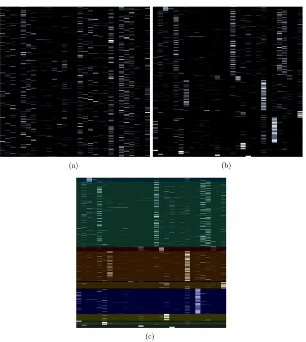
from the clustering [71]. Later, the number of clusters is used for the number of components for the GMM procedure and the associated set of pixels are used in the estimation procedure. An example abundance matrix, the resulting clusters, and the pixels associated with these clusters from our experiments are shown in Figure 3.2 and Figure 3.3.

Advantage of this method is that it automatically determines the number of clusters K. Disadvantages of the method are that it performs considerably slower

(a) (b)

(c)

Figure 3.2: Hierarchical clustering examples from our experiments on the abun-dance feature space. (a) Raw abunabun-dance matrix. (b) Rearranged abunabun-dance matrix. (c) Rearranged hierarchical clustering result.

(a)

(b)

(c)

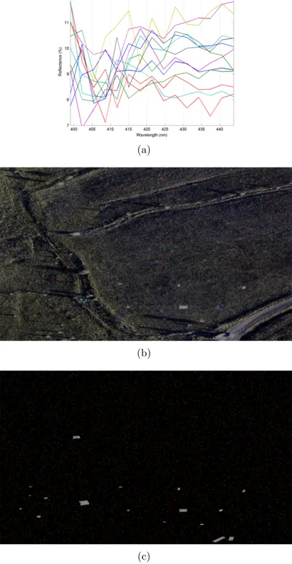
Figure 3.3: Hierarchical clustering examples from our experiments on the image feature space. (a) Mean vectors of the clusters. (b) Pixels associated with the 3 clusters that have the highest coverage are overlayed on the RGB image. (c) Pixels associated with the 3 clusters that have the highest coverage are overlayed on the ground truth image.

than the other methods for identifying the dominant background groups, and the K selection algorithm and the linkage criterion may not be perfectly suitable for all clusters of interest.

3.3.3

BiClustering

The last method we use is biclustering that simultaneously clusters both rows and columns of a data matrix, which in our case is the fractional abundance matrix X. With hierarchical clustering, we were aiming to cluster the observa-tion pixels based on the assumpobserva-tion that endmembers tend to appear together at the sub-pixel level. However, by doing so, we could only cluster the pixels but not the endmembers. One can interpret the list of endmembers appearing together in a mixture as an ingredient list. If the problem was to cook a soup, the ingredients required to cook the named soup would be predetermined. Even though the amount of how much from an ingredient was put in the soup could vary at small scales, the list would stay the same. For our problem, the soup is the complex background component and the ingredients are our endmembers. By analysing the fractional abundance matrix X we hope to identify the list of all soups (components) that are present on the table (image) by extracting the information on which ingredients tend to be favored together in order to make a tasty soup.

The biclustering algorithm simultaneously clusters the rows and columns as follows. The singular value decomposition,

X = UΣVT_{, (3.14)}

where Σ is an M ×N rectangular diagonal matrix that has non-negative real num-bers on the diagonal, the columns of U ∈ RM ×M and the columns of V ∈ RN ×N are right and left singular values respectively, provides the partition informa-tion of the rows and columns for a given abundance matrix X ∈ RM ×N_{. The}

singular vectors are first ranked based on their ability to be approximated by a piecewise-constant vector. In which case, the scores are obtained by using Euclidean distance to measure the error for individual approximations that are

Figure 3.4: BiClustering example of rearranged biclusters that reveal a checker-board structure. Taken from the official Scikit-Learn web page [2].

found by using one-dimensional k-means. Later, the partitioning of the rows is performed by projecting the rows of the abundance matrix X to V, such as XV, followed by a k-means clustering. Similarly, the partitioning of the columns is performed by projecting the columns of the abundance matrix X to U, such as XT_{U, followed by a k-means clustering. Resulting labels are the row and column}

labels respectively [72]. To solve the biclustering problem, we used the Spectral Biclustering algorithm within the machine learning package Scikit-Learn [2].

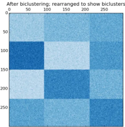
After the biclustering procedure, we obtain clusters consisting of several rows and columns assigned to them. To visualize the output, one can rearrange the data matrix to obtain contiguous clusters. Based on the setting, individual rows and columns might be assigned to a single cluster, or the same rows and columns might be assigned to multiple clusters. In the first case, the data matrix can be rearranged to reveal the clusters along the diagonal. For the latter case, a checker-board structure is revealed after rearranging as in Figure 3.4. In this thesis, the latter case is considered as we cluster pixels and endmembers simultaneously, and neither of them are necessarily restricted to belong in one cluster as the same in-gredient could be used for multiple soups or vice versa. An example abundance matrix, the resulting clusters, and the pixels associated with these clusters from our experiments are shown in Figure 3.6 and Figure 3.5.

(a) (b)

(c)

Figure 3.5: BiClustering examples from our experiments on the abundance fea-ture space. (a) Raw abundance matrix. (b) Rearranged abundance matrix. (c) Rearranged biclustering result.

(a)

(b)

(c)

Figure 3.6: Biclustering examples from our experiments on the image feature space. (a) Mean vectors of the clusters. (b) Pixels associated with the 3 clusters that have the highest coverage are overlayed on the RGB image. (c) Pixels associated with the 3 clusters that have the highest coverage are overlayed on the ground truth image.

Advantage of the method is that it simultaneously clusters pixels and endmem-bers, which allows a better identification of the complex background components that consist of endmembers that are in mixture with each other at the sub-pixel level. However, a disadvantage of the method is that the number of clusters for rows and columns need to be specified. Another disadvantage is that this step involves randomness due to the random initialization of the k-means procedure. All of the other methods can produce the same result for any run.

We will describe the experimental setups and compare the three methods for identifying the dominant background groups in Chapter 4.

3.4

Probabilistic Background Modeling

The anomaly detection problem consists of efficient and correct modeling of an image background so the anomalies can be identified as outliers with respect to this model. In this thesis, we are focused on the identification of anomalies in heterogeneous scenes with multiple classes of materials being present at the sub-pixel level in the background. Within the previous subsections we have explained how we exploit the spectral characteristics in an image by applying unmixing and how we identify the dominant background groups. The transition to abundance feature space took place with unmixing, and the consecutive steps were performed on this feature space. The probabilistic background modeling step, on the other hand, will happen in the image space with the original spectral bands, while utilizing the information harnessed from the previous steps such as the number of background components and the initial sets of pixels representing them.

For the background modeling, we use Gaussian Mixture Models (GMM). Given K components, as it was learned from the previous step, the mixture of individual components’ densities is formulated as

p (y|Θ) = K X k=1 αkpk(y|θk) , (3.15) θ = {µ , Σ } (3.16)

where Θ = (α1, . . . , αK, θ1, . . . , θK) such that αk ≥ 0 and K

P

k=1

αk= 1.

α1, . . . , αK are called the mixing parameters and pk(y|θk) is the component

den-sity. µ is the mean and Σ is the covariance matrix.

3.4.1

Initialization

One of the main contributions of this paper is the initialization of the Gaussian Mixture Model components using the dominant background groups learned from the previous steps. The three important parameters estimated are

• the number of components (K), • the mean of components (µ), • the covariance of components (Σ).

The number of components K is the number of dominant endmembers learned for the thresholding method and the number of clusters for the hierarchical clustering and biclustering methods. Given the dominant background groups, the mean for each component is initialized as

µ_k= 1 |Ck|

X

a∈Ck

y_a (3.17)

where Ck is the set of pixels associated with the component k. The covariance

matrix Σk is initialized as Σk = 1 |Ck| − 1 X a∈Ck (y_a− µ_k)(y_a− µ_k)T. (3.18)

3.4.2

Expectation Maximization (EM)

After the initializing step, the Expectation Maximization (EM) is used to obtain the final background model estimates. The motivation of using EM is the pos-sibility of estimation errors due to the fact that the number of pixels associated

with each component is variable. Although the minimum size of the said set of pixels is controlled by a threshold based on the desired maximal size of an anomaly, the estimations are still only valid as a basis for the EM procedure to avoid local optima. The stopping condition for the EM procedure is based on the change in log-likelihood between two iterations and a predetermined maximum number of iterations. The log-likelihood at a given iteration is given by

log L(Θ|Y) = X y∈Y log K X k=1 αkpk(y|θk) ! . (3.19)

3.5

Partition Combination

The goal is to compute p(anomaly|y) for each pixel y so that a detection can be made as

pixel y is anomaly if p(anomaly|y) > τ. (3.20) We are given probabilistic background models ps(ys|Θs) estimated for individual

partitions s = 1, . . . , S as described in the previous sections. We would like to combine these models into a final background model p(background |y) so that the anomaly probabilities in (3.20) can be obtained as

p(anomaly|y) = 1 − p(background |y) (3.21) where

p(background |y) = p(y|background )p(background ) p(y)

= p(y|background )p(background )

p(y|background )p(background ) + p(y|anomaly)p(anomaly). (3.22) Since the full anomaly distribution p(y|anomaly) is unknown and the prior prob-abilities p(anomaly) and p(background ) are difficult to estimate, we aim to ap-proximate p(background |y) from p(y|background ). Following the reasoning in [73] and the Bayesian combination methods in [74], p(y|background ) can be ap-proximated from the probabilities computed from the individual partitions as p (y |Θ ), . . . , p (y |Θ ) by using the following combination rules:

• Product rule: p(y|Θ1, . . . , ΘS) ∝ S Y s=1 ps(ys|Θs) (3.23)

will favor extreme values, such that, if a pixel is given a very low probability of being background from any partition, the final probability for the same pixel will be very low.

• Sum rule: p(y|Θ1, . . . , ΘS) ∝ 1 S S X s=1 ps(ys|Θs) (3.24)

averages the values from the partitions, and provides a combination that is more robust to variations in the probabilities given by different partitions. • Max rule:

p(y|Θ1, . . . , ΘS) ∝ max

s ps(ys|Θs) (3.25)

will consider a pixel as a member of the background class if any of the partitions give a high probability for the pixel.

• Min rule:

p(y|Θ1, . . . , ΘS) ∝ min

s ps(ys|Θs) (3.26)

will consider a pixel as a member of the background class if and only if all of the partitions give a high probability for the pixel.

For the experiments, we used the min rule since we are interested in the anoma-lies that are not necessarily apparent on all the spectral partitions, but more focused on finding all the anomalies that stand out from their surroundings on different regions of the spectrum.

After the combination, a post processing step is used in an attempt to re-duce the false alarm rating. For this purpose, a structuring element with a size determined by the minimal area of an expected anomaly is defined. With this structuring element, opening by reconstruction of the probability image is per-formed to eliminate the detections that are smaller than the expected size of an anomaly. The resulting probability image is then applied to a constant false alarm rating adaptive threshold to retrieve the final set of pixels identified as anomalies.

Chapter 4

Experiments

4.1

Dataset

The proposed methodology is evaluated using an airborne hyperspectral image. An anomaly detection scenario was prepared by placing different materials such as fabrics, carpets, wooden sheets, floor tiles, etc., on a natural landscape back-ground in Turkey. The scene also has two cars that can be considered as anoma-lies. The image that was acquired with a visible and near infrared camera from an altitude of 500 m contains 1500 × 885 pixels and 182 bands covering the spectral range from 399 nm to 978 nm with a spatial resolution of 16 cm. Data collection and atmospheric correction were performed by Havelsan, Inc. The ground truth was prepared by manual delineation of 19 objects in the scene. The sizes of the objects vary between 4 and 900 pixels where 14 of them are smaller than 180 pixels. The RGB image and the corresponding ground truth mask are shown in Figures 4.1 and 4.2, respectively. The list of all the ground truth objects in the scene and the corresponding sizes in pixels are shown in Table 4.1.

We are using two spectral signature libraries, namely, the Havelsan Spectral Library and the USGS Spectral Library. The first spectral library (Havelsan Spectral Library) used in the experiments contains 29 signatures acquired with

Figure 4.1: RGB image.

a spectrometer in the same scene as well as in other scenes under different at-mospheric conditions. The second spectral library (USGS Spectral Library) [67] contains 794 spectral signatures acquired with a set of different spectroscopy in-struments. For experimental purposes, the spectral signatures were selected based on their quality and wavelengths range specified by the USGS Spectroscopy Lab. The spectral signatures for both libraries were applied to an interpolation step to match the wavelengths of the hyperspectral image. The ground truth object boundaries are overlaid as red contours on binary masks.

4.2

Baseline Methods

For the baseline methods to serve as a comparison basis in our experiments, we used the RX anomaly detector that is built by using the full spectrum and another detector named RX-GMM that replaces the Gaussian in the RX framework by a GMM that is built by using 8 Gaussian components estimated using 10 PCA components that retain 98% of the variance in the full data.

Figure 4.2: Binary mask of 19 small objects.

Table 4.1: Ground truth objects in the scene. Name Size 1 Car #1 427 2 Car #2 742 3 White Linoleum 137 4 Clothing #1 924 5 Graybody 40 6 Clothing #2 121 7 Laminated Flooring 61 8 Blue Carpet 132 9 Blue Styrofoam 82 10 Clothing #3 8 11 Brown Carpet 104 12 Clothing #4 54 13 Ceramic Tile 83 14 Clothing #5 179 15 Black Linoleum 174 16 Black Nylon 71 17 Spektralon 4 18 Tyvek #1 536 19 Tyvek #2 456

4.3

Results

Due to the computational limitations, the data was sampled before the clustering procedures. For the hierarchical clustering 50000 pixels, and for the biclustering 100000 pixels were randomly selected. For the thresholding based method, the abundance threshold ta was set to 0.1 for the Havelsan Spectral Library and 0.04

for the USGS Spectral Library, and the coverage threshold tc was set to 0.17

empirically. For the hierarchical based method, the free parameter that controls the automatic determination of the number of clusters in the algorithm in [71] was set to 9 for Havelsan Spectral Library and 3.8 for the USGS Spectral Library empirically. For the biclustering based methods, the number of clusters for the endmembers is set to 10 for the Havelsan Spectral Library and 50 for the USGS Spectral Library, and the number of clusters for the pixels is set to 15 for both cases empirically.

Visual and numeric outputs from both the baseline and the proposed meth-ods are categorized in the following subsections. In both subsections, the log-probability anomaly map provided by the method and the binary mask for the detection result are included. The binary masks represent the top 0.20% of the pixels in the corresponding log-probability anomaly maps. This number is se-lected based on the total number of pixels that are representing the anomalous objects in Figure fig:geredegt to reflect the abilities of corresponding methods on very low false alarm ratings. Experimental results for the proposed methods for identifying the dominant background groups are provided inside individual subsections. Furthermore, the results before post-processing are also included for reference.

4.3.1

Baseline Methods Results

Experimental results for the baseline method RX algorithm before post-processing are shown in Figure 4.3.

(a)

(b)

Figure 4.3: Anomaly detection results for the RX detector before post-processing. (a) Log-probability anomaly map. (b) Binary detection map.

Experimental results for the baseline method RX algorithm after post-processing are shown in Figure 4.4.

(a)

(b)

Figure 4.4: Anomaly detection results for the RX detector after post-processing. (a) Log-probability anomaly map. (b) Binary detection map.

Experimental results for the baseline method RX-GMM algorithm before post-processing are shown in Figure 4.5.

(a)

(b)

Figure 4.5: Anomaly detection results for the RX-GMM detector before post-processing. (a) Log-probability anomaly map. (b) Binary detection map.

Experimental results for the baseline method RX-GMM algorithm after post-processing are shown in Figure 4.6.

(a)

(b)

Figure 4.6: Anomaly detection results for the RX-GMM detector after post-processing. (a) Log-probability anomaly map. (b) Binary detection map.

4.3.2

Havelsan Spectral Library Results

Experimental results for the proposed thresholding based method before post-processing are shown in Figure 4.7.

(a)

(b)

Figure 4.7: Anomaly detection results for Havelsan Spectral Library and the thresholding based method before post-processing. (a) Log-probability anomaly map. (b) Binary detection map.

Experimental results for the proposed thresholding method after post-processing are shown in Figure 4.8.

(a)

(b)

Figure 4.8: Anomaly detection results for Havelsan Spectral Library and the thresholding based method after post-processing. (a) Log-probability anomaly map. (b) Binary detection map.

Experimental results for the proposed hierarchical clustering based method before post-processing are shown in Figure 4.9.

(a)

(b)

Figure 4.9: Anomaly detection results for Havelsan Spectral Library and the hierarchical clustering based method before post-processing. (a) Log-probability anomaly map. (b) Binary detection map.

Experimental results for the proposed hierarchical clustering based method after post-processing are shown in Figure 4.10.

(a)

(b)

Figure 4.10: Anomaly detection results for Havelsan Spectral Library and the hierarchical clustering based method after post-processing. (a) Log-probability anomaly map. (b) Binary detection map.

Experimental results for the proposed biclustering based method before post-processing are shown in Figure 4.11.

(a)

(b)

Figure 4.11: Anomaly detection results for Havelsan Spectral Library and the biclustering based method before post-processing. (a) Log-probability anomaly map. (b) Binary detection map.

Experimental results for the proposed biclustering based method after post-processing are shown in Figure 4.12.

(a)

(b)

Figure 4.12: Anomaly detection results for Havelsan Spectral Library and the biclustering based method after post-processing. (a) Log-probability anomaly map. (b) Binary detection map.

4.3.3

USGS Spectral Library Results

Experimental results for the proposed thresholding based method before post-processing are shown in Figure 4.13.

(a)

(b)

Figure 4.13: Anomaly detection results for the USGS Spectral Library and the thresholding based method before post-processing. (a) Log-probability anomaly map. (b) Binary detection map.

Experimental results for the proposed thresholding method after post-processing are shown in Figure 4.14.

(a)

(b)

Figure 4.14: Anomaly detection results for the USGS Spectral Library and the thresholding based method after post-processing. (a) Log-probability anomaly map. (b) Binary detection map.