Parallelization of the fast multipole solution of the electromagnetic scattering problem

P A R A L L E L IZ A T IO N O F T H E F A S T M U L T IP O L E

S O L U T IO N O F T H E E L E C T R O M A G N E T IC

S C A T T E R IN G P R O B LE M

A THESIS

SUBMITTED TO THE jgEPARTMENT OF COMPUTER

ENGINEERING AND INFORMATION SCIENCE

AND THE INSTITUTE OF ENGINEERING AND SCIENCE

OF BILKENT UNIVERSTY

IN PARTIAL FULFILLMENT OF THE REQUIREMENTS

FOR THE DEGREE OF

MASTER OF SCIENCE

By

All Ayub M.Kalufya

September 1997

PARALLELIZATION OF THE FAST MULTIPOLE

SOLUTION OF THE ELECTROMAGNETIC

SCATTERING PROBLEM

A THESIS

SUBMITTED TO THE DEPARTMENT OF COMPUTER ENGINEERING AND INFORMATION SCIENCE AND THE INSTITUTE OF ENGINEERING AND SCIENCE

OF BILKPNT UNIVERSITY

IN PARTIAL FULFILLMENT OF THE REQUIREMENTS FOR THE DEGREE OF

MASTER OF SCIENCE

By

All Ayub M . Kalufya September, 1997

é é Ç ' К З Т

I certify that I have read this thesis and that in my opinion it is fully adequate, in scope and in quality, as a thesis for the degree of Master of Science.

Assoc. Prof. C w det Aykanat (Advisor)

I certify that I have read this thesis and that in my opinion it is fully adequate, in scope and in quality, as a thesis for the degree of Master of Science.

I certify that I have read this thesis and that in my opinion it is fully adequate, in scope and in quality, as a thesis for the degree of Master of Science.

Asst. Prof. Tuğrul Dayar

Approved for the Institute of Engineering and Sciences:

Prof. Mehmet Baray^

ABSTRACT

P A R A L L E L IZ A T IO N O F T H E FAST M U L T IP O L E S O L U T IO N O F T H E E L E C T R O M A G N E T IC S C A T T E R IN G

P R O B LE M

Ali Ayub M. Kalufya

M .S. in Computer Engineering and Information Science Supervisor: Assoc. Prof. Cevdet Aykanat

September, 1997

The solution to the electromagnetic scattering problem may be modelled as an iV-body problem. Using this model this work develops a solution that is based on a specific variant of the Fast Multipole algorithm that was proposed by V. Rokhlin[17] and modified furttier by Anderson[3], that is the Fast Multipole Method without multipoles. Because an iterative scheme is used, we also de­ velop an preconditioning algorithm that is especially tailored for the solution of problems that may be modelled using Af-body concept.

Moreover, in this work parallel computing is employed to improve the solu­ tion even further by developing a program that will utilize the above mentioned fast multipole method concept in parallel so as to be able to solve even larger and more interesting real-life problems in a reasonable amount of time and using minimum possible memory space.

A parallel version of the fast multipole method is developed and imple­ mented on the Parystec Coignitive Computer 24 node multicomputer using the single program multiple data paradigm for solving the electromagnetic scattering problem in 2 dimensions.

Key words:

Preconditioning

N -body Concept, Fast Multipole Method, Blockwise Sparse

ÖZET

E L E K T R O M A N Y E T İK SAÇ ILIM P R O B LE M İN İN HIZLI M U L T IP O L E Ç Ö Z Ü M Ü P A R A L E L İST İR İLM E Sİ

Ali Ayub M . Kalufya

Bilgisayar ve Enformatik Mühendisliği Bölümü Yüksek Lisans Tez Yöneticisi: Doç. Cevdet Aykanat

Eylül, 1997

Elektromanyetik saçılım probleminin çözümü A^^-body problemi ile modellenebilir. Bu çalışmada bu modeli kullanarak V. Rokhlin [17] tarafından önerin ve An- derson [3] tarafından geliştirilen Hızlı Multipole Algoritmasının bir uyarlama olan bir çözüm üretir : Multipolesuz Hızlı Multipole Metodu. Inelemeli bir yöntem kullanıldığından, özellikle A/^-body kavram kullanilarak modellenebilen problemlerin çözümü tüm üretilmiş bir ön-şartkandirma algoritması geliştridik.

Bu çalışmada, paralel hesaplama, daha enteresan ve büyük gerçek hayat problemlerini mâkûl bir zamanda ve olasi minimum hafıza alanı kullanarak çözebilmek için yukarda bahsedilen hızhmultipole metodu paralelistiren bir program geliştererek çözümü daha da ilerletmek için kullanıldı.

Hızlı Multipole Metodunun paralel bir uyarlama iki boyutta elektromayetik saçılma problemini çözmek için, tekli program çoklu data yöntemi kullanilarak Parytec Coignitive Computer 24 düğümü da geliştirdi ve uygulandı.

Anahtar sözcükler: Y -b od y kavramı, Hızlı Mültipole Metodu, Seyrek Blok On-sartlandırması.

ACKNOWLEDGEMENT

I am mostly grateful to Dr. Aykanat and Dr. Gürel for suggesting this interesting research topic. Sincerely, they have been supervis­ ing me with patience and everlasting interest all the way through the period of my graduate studies.

I am also indebted to Dr. Gürsöy and Dr. Kurç for showing keen interest to the subject matter. Their remarks and recommendations have been very constructive.

I have to express my gratitude to the technical and academic staff of Bilkent University. I am especially thankful to my classmates of my first graduate year in general, and my office mates in particular. Lastly, albeit of most significance, I express my sincere recognition for maybe the most important role played by my wife throughout this work; without her warm motivation and concern maybe this would never be a reality.

Contents

1 Introduction 1

1.1 B a c k g ro u n d ... 1

1.2 The A/^-Body Problem 2 1.3 Fast Algorithms for the A/^-body P ro b le m ... 3

1.4 Organization of the T h e s is ... 4

2 The Electroniagnetic Scattering Problem 7 2.1 The Physical M o d e l... 7

2.2 The Mathematical M o d e l... 8

3 The Fast Multipole Method 10 3.1 O verview ... 10

3.2 Informal Description of the FMM A lg o rith m ... 12

3.3 Computational Foundations of the F M M ... 13

3.3.1 The A/’-body M o d e l... 14

3.3.2 Original Fast Multipole M e t h o d ... 15 vii

3.3.3 The Anderson’s Fast Multipole M e th o d ... 17 3.3.4 The Fast Multipole Method for the Scattering Equation . 19

4 The Sequential Implementation of the Scattering Solution 22

4.1 In trodu ction ... 22 4.2 Common Features of the FMM Implementations... 24 4.3 Speeding up the Matrix Vector Multiplication 25 4.4 The Original Sequential Implementation 26

4.4.1 Features of the Original Im p lem en tation ... 28 4.4.2 The Original Sequential Matrix Vector Multiplication

A lg o r ith m ... 29 4.5 Modifications to the Original Sequential Algorithm 31 4.5.1 From Static to Dynamic Memory M anagement... 31 4.5.2 Cache U tiliza tion ... 31 4.5.3 Reduction of Loop C om putation... 32 4.5.4 Reduction of Indexing 32 4.5.5 Changes on the Preconditioner 32 4.6 The Modified Sequential Im plem entation... 33 4.6.1 Features of the Modified Im plem entation... 33 4.6.2 The Modified Sequential spMx V Algorithm 34

5 Data Organization for the spMx VAlgorithm 37

5.1 Data Parallelism of the spMx V A lg o r ith m ... 37

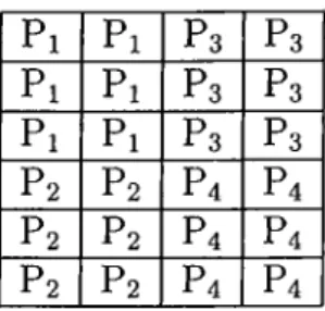
5.1.1 All nearfield blocks kept on a single processor 38 5.1.2 The Block Checkerboard Partitioning... 38

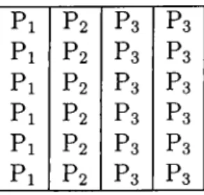
5.1.3 The Block Columnwise Partitioning... 40

5.1.4 The Block Rowwise Partitioning... 41

5.2 Data P artition in g... 41

5.2.1 Graph Theoretic Modelling of the Z/vf M a tr ix ... 43

5.2.2 Implementation Considerations 44 6 The Parallel Solution to the Scattering Problem 46 6.1 Parallelization of the spMx P R ou tin e... 47

6.2 The Parystec Cognitive Computer C C -2 4 ... 48

6.2.1 Physical Topology of the Parystec C C -2 4 ... 48

6.2.2 Communication Primitives of the Parystec CC-24 . . . . 49

6.3 The Parallel spMx V A lg o r it h m ... 49

6.4 Preconditioning the Solution Strategy... 52

6.4.1 Development of the Factorization A lg o r ith m ... 54

7 Analysis of the Experimental Results 60 7.1 Timing R e s u l t s ... 61

7.2 The time for a single ite r a tio n ... 61

7.3 Number of Ite ra tio n s... ... 64

CONTENTS

7.4 Parallel Efficiency and S p e e d u p ... 66 7.5 P recon dition in g... 69

8 Conclusion 74

8.1 Final Rem arks... 74

8.2 Similar Work 75

8.3 Future W o r k ... 75

A Mathematical Modelling of the Fast Multipole Method 77

A. 1 The A -b o d y M o d e l ... 77 A .2 Derivation of the Multipole Expansion 78 A.3 Error Bounds of a Multipole E xpansion... 79 A .4 Derivation of the potential sum using Anderson’s F M M ... 79

List of Figures

4.1 The Conjugate Gradient Squared Algorithm... 27 4.2 The Original Sequential Matrix Vector Multiplication {spMx V)

A lg o r ith m ... 30 4.3 The Modified Sequential Matrix Vector Multiplication (spMx V)

A lg o r ith m ... 36

6.1 The Parallel Matrix Vector Multiplication (spMx V) Algorithm . 56 6.2 The Ring Expand A lgorith m ... 57 6.3 The Memory Hierachy 57 6.4 The Proceeding of Blockwise Sparse Matrix Factorization . . . . 58 6.5 The Blockwise Sparse Factorization A lg o rith m ... 59

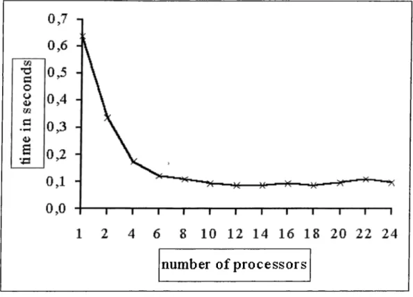
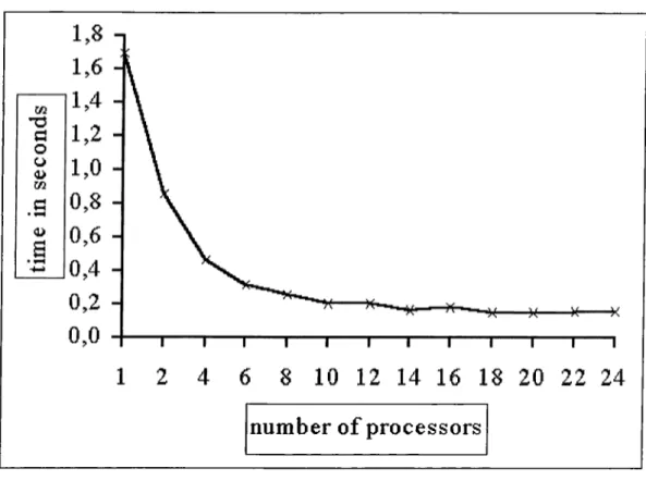
7.1 Time for one iteration in the solution of the 36 clusters problem 64 7.2 Time for one iteration in the solution of the 50 cluster problem . 65 7.3 Time for one iteration in the solution of the 111 cluster problem 66 7.4 Number of iterations required for solutions of the 36, 50 and 111

clusters p r o b le m s ..., ... 67

7.5 The complete solution time for the 36 cluster p rob lem ... 68 7.6 Time for complete solution of the 50 clusters problem... 69 7.7 Time for complete solution of the 111 clusters problem 70 7.8 The speedups attained in solving the 36, 50, and 111 clusters

p roblem s... 72 7.9 The variation of the efficiency of the parallel scattering solution. 73

List of Tables

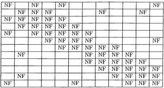
4.1 The Structure of Interaction Matrix for a 12 Cluster Problem 35

5.1 The Checkerboard Partitioning 39 5.2 The Columnwise Partitioning 40 5.3 The Rowwise P a r titio n in g ... 41

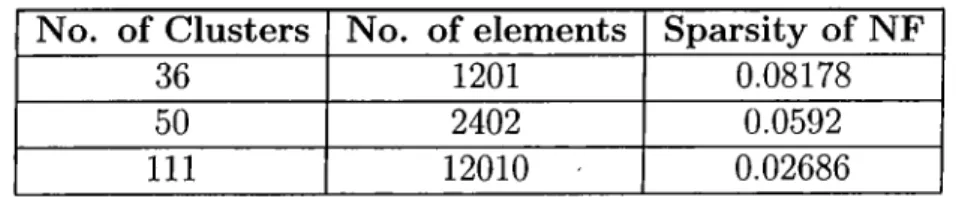
7.1 The characteristics of the electromagnetic scattering problems

)

solved in these experiments 60 7.2 Timing results for the 36 clusters problem 61 7.3 The timing results for the 50 cluster p rob lem ... 62 7.4 Timing results for the 111 cluster p r o b le m ... 62 7.5 The comparison between factorization time of the Sparse library

spFactor and our new Blockwise sparse factorization algorithm . 71 7.6 The problem solution time (factorization+looping to conver­

gence) of the Sparse library spFactor compared to our new Block- wise sparse factorization algorithm 71 7.7 The comparison between running time per a single loop of the

original implementation and the new modified implementation . 71

Chapter 1

Introduction

1.1

Background

Numerical simulation and analysis of the electromagnetic scattering phenom­ ena is used in several engineering applications to gain important information about the systems prior to their (actual implementation. However, due to the limitations in computing power and vast amounts of data and time necessary to acquire high simulation results, the size of the problem that can be solved using conventional methods is very much limited.

In this work the Fast Multipole Method is investigated, particularly its use in the above mentioned simulations to reduce both the space and time complexities of the simulations. A particular serial (sequential) implementation of the algorithm is examined aiming at improving it into producing even much better performance in terms of time and space requirements. Moreover, a sparse block matrix factorization is designed and implemented so as to exploit maximally the structural nature of the interaction matrix.

Finally, a parallel version of the improved algorithm is designed and im­ plemented on the Parystec CC 24 node multicomputer to allow for even very much larger data sets, and to perform the calculations within reasonable time

CHAPTER 1. INTRODUCTION

scales.

1.2

The A/^-Body Problem

The electromagnetic scattering phenomena is a special case of a more generic A/’-body problem. An A -bod y is a collection of N particles each of which being acted upon by the remaining N —1 particles hence making the amount of computational effort required to evaluate the total force acting on each particle be of order If we calculate the interactions using the pairwise law, then the amount of work becomes of order — N) which is asymptotically the same 0{N'^) [18]. This computation is prohibitively expensive for large N which is common for real-life problems due to the amount of storage and time required to compute the interactions.

The basic notion behind the A -bod y is that a cluster of distant particles is replaced by a single pseudo-particle, and that as the distance to the cluster increases, the amount of particles that may together be considered as a single pseudo particle may increase. The quantity of interaction exerted by nearby particles is approximated by their interaction with this pseudo-particle.

In real-life there is a big variety of physical problems that can be modelled as a collection of interacting bodies or particles. Instances of this A -bod y prob­ lem can be perceived in computational fluid mechanics, molecular dynamics, plasma physics where the bodies may be ions and electrons, and astrophysics where the bodies may be stars [4].

Elsewhere [9], the A -bod y concept has been applied into speeding the matrix-vector multiplication which is a bottleneck in the iterative scheme that is used to solve the scattering solution. In chapter 2, a description of model­ ing of the scattering problem as an A -body, the model on which a particular variant of an A -b od y algorithm, the Fast Multipole Method, is used to speed up its computation. Moreover, the whole FMM based solution strategy is par­ allelized so as to be able to exploit its inherent parallel nature and utilize the

CHAPTER 1. INTRODUCTION

modern high performance computing parallel architectures made available by the current developments of technology.

1.3

Fast Algorithms for the A-body Problem

To speed up the A -bod y computation we can reduce either the frequency with which the force at an individual particle is calculated, or the computational cost of calculating the force per particle. There are several methods [12] [3] developed based on these strategies. These, including now historical algo­ rithms such as the particle/mesh algorithms developed about 20 years ago, use approximations to calculate the interactions to reduce the execution time sig­ nificantly. However, the performance of A -bod y computation may be improved even further by exploiting the inherent parallelism within the fast summation technique.

The Grengard-Rokhlin algorithm [10], termed the Fast Multipole Method, is the first N-Body algorithm in which the truncation error is controllable and could be fine tuned to produce a specified precision. In the FMM the pseudo particle is represented by an infinite multipole expansion centered on a sphere which contains the entire cluster. This expansion is truncated to a finite number of terms, where the number of terms taken in each expansion controls the precision. Forces may be evaluated to machine precision if required, and for a large number of particles this method can be even more accurate than the direct summation technique.

Due to its reduced computational complexity and memory requirement, the FMM can be used for problems demanding a high number of particles and a high controllable precision. The basis of this work [11] is the application of FMM in the Fast Radar Cross Section computation of large canonical two di­ mensional geometries. In this application, the electromagnetic scattering from two-dimensional canonical conducting strip geometries is analyzed. Although the original objective of this work was to parallelize the existing sequential

CHAPTER 1. INTRODUCTION

solution, prior to parallelization the existing sequential solution was improved for better performance.

A method of frequent choice for computing scattering cross sections and radiation patterns is to solve a matrix equation, Z x I — V , derived from the discretization of an integral equation [18]. The number of unknowns required for accurate modelling of such problems can be very large, which severely limits the problem size. The system can be solved by factorizing the dense matrix Z, an 0{N^) operation, or by using an iterative method which generally requires 0 { N ‘^) operations per an iteration. In this work we use a combination of the two, that is, the dense matrix Z is considered to be a sum of two matrices, a sparse matrix Z^p due to the near field interaction and a dense matrix Zpp due to the interactions between particles in far clusters and Zj^p is factorized and used as a preconditioner in the iterations for which FMM is used twice to perform a fast matrix-vector calculation of the product of Zpp and the current guess solution vector.

The initial work was done on the sequential code [11] to improve both its speed and memory constraints. Then to utilize the parallelism in the algorithm, the algorithm was parallelized and implemented on the Parsytec CC 24 node multicomputer. Moreover, to exploit the peculiar blockwise sparse property of the matrix resulting from the model, a blockwise sparse preconditioner was developed to speed up the convergence of the iterative process involved in the solution.

1.4

Organization of the Thesis

In this thesis the fast multipole method is investigated and used to solve a certain electromagnetic scattering problem in parallel. The thesis starts with a detailed description of the electromagnetic scattering problem in Chapter 2. The chapter throws light on the mathematical modelling of the scattering problem in such a way that the problem conforms to the characteristics of the

CHAPTER 1. INTRODUCTION 5

N-body computational paradigm.

In chapter 3 the fast multipole method is described. Here the computa­ tional model of the original FMM is explained together with the mathematical foundations of the generic multipole expansions. Moreover, the transition from the use of multipole expansions of the original Grengard-Rokhlin FMM algo­ rithm to the use of Poisson expansions in Anderson’s FMM without multipoles is discussed. Moreover the comparison between the two similar algorithms as far as computation and programming complexity is concerned is also discussed in this chapter.

Chapter 4 concentrates on the sequential solution to the electromagnetic scattering problem. A particular implementation [11] is discussed in detail to highlight various advantages and disadvantages of the Anderson’s method and this particular application. For reasons explained in the chapter more emphasis is given to the matrix vector multiplication. In Chapter 4 the narration of the modifications made as part of this thesis work towards improving both time and memory efficiency of the basic implementation are given. Finally, a description is given of the modified sequential implementation that is developed in this work. Actually, this modified version is the actual basis of the parallelization efforts done in this work.

In Chapter 5 the possible strategies that can be used for distribution of data among processors in a parallel program are examined and the strategy used in this solution is described. Moreover, the method that is used in this work to create a load balance among the processors is explained. This method is based on a more generic graph partitioning algorithm.

Our parallelization strategy and its particular implementation is given in Chapter 6. Chapter 6 explains the methodologies that are used to reach the parallel algorithm and discuss the reasons for adopting such methods. More­ over, it describes the parallel spMx V and the blockwise sparse factorization algorithms that were developed as part of this work.

CHAPTER 1. INTRODUCTION

Chapter 7 is devoted to the experiments that were conducted to test the per­ formance of both the original and modified sequential implementations together with the subsequent parallel implementation of the modified version. More­ over, it highlights various physical and computational aspects of the Parystec CC-24 and use them to explain the experimental results

In the closing chapter remarks and conclusions that are derivable from the experiments conducted as part of this work are discussed together with the vision about what is to be expected in the future as far the Fast Multipole Method is concerned especially on its application on solving the electromag­ netic scattering problem and the more generic A -bod y problem.

Chapter 2

The Electromagnetic Scattering

Problem

The electromagnetic scattering by two dimensional conducting cylinders is a classical electromagnetic problem and quite a number of algorithms have been developed to solve it. In most cases, the problem is modelled as a matrix equation where the unknown is the induced current. The matrix equation may be solved directly using the Method of Moments (MOM) which requires 0{N^) if the Gaussian Elimination is used to invert the interaction matrix. If an iteration scheme such as the Conjugate Gradient Squared (CGS) method is used the complexity becomes that of the matrix-vector in the iteration, that is 0 { N ‘^) per iteration. However, in the case of the iterative scheme it is of importance that the convergence rate be maintained as much as possible.

2.1

The Physical Model

In the electromagnetic scattering an individual metallic scatter can be decom­ posed into N subscatters. When an electromagnetic wave falls incident on a subscatter, the subscatter will carry a current distribution which is determined

CHAPTER 2. THE ELECTROMAGNETIC SCATTERING PROBLEM

by a discretized integral equation that is determined by the equation express­ ing interaction between subscatters. Therefore, for the numerical solution to obtain the field at a subscatter due to other subscatters one need N multipli­ cations, and since there are N subscatters multiplications are needed to compute their total interactions between them. This is in complete confor­ mity to the A -b o d y problem and hence shows the electromagnetic scattering problem as a special case of the more general A -b od y problem.

2.2

The Mathematical Model

In this section we describe the procedure by which an electromagnetic scatter­ ing problem may be modelled into a matrix equation.

The surface integral that governs that scattering solution is given by io .« ,

IdS'gAp -

p

'JM

p

')

-E 'rM

P<^S

2

1

9o{p - Po) = \p - Pol) (2.2)

and J z { p ') is the induced current on the surface of the scatter and is

the incident field.

The equation (1) above is then discretized into [18]

where and 9ij — (2.3) (2.4) b, = E r ( P i )

CHAPTER 2. THE ELECTROMAGNETIC SCATTERING PROBLEM

The result is a matrix equation

Z x I = V (2.5) which may be solved either directly using Gaussian elimination at the cost of 0{N^) operations, or iteratively at a cost of one or more matrix-vector op­ erations which is order 0(A /’^) operations per an iteration. In this work the Conjugate Gradient Squared iterative scheme is used to solve equation (2.5) and a fast summation algorithm that is based on the Fast Multipole Method is used to reduce the time complexity of the matrix vector multiplication op­ eration from 0 { N ‘^) to . Moreover, a blockwise sparse factorization is used to supply a preconditioner matrix to improve the convergence rate of the iteration.

Chapter 3

The Fast M ultipole M ethod

3.1

Overview

Several efforts are documented that aim at reducing the complexity of the N- body problem, among these being the particle-in-cell methods that has been used with some success in plasma physics [22]. These methods have a generic complexity of 0 { N + M l o g M ) , where N is the number of interacting par­ ticles and M is the number of mesh points of the iV-body. The number of mesh points is normally chosen to be proportional to the number of parti­ cles, but with a small constant of proportionality so that M ^ V so as to make the asymptotic complexity be of order 0 { N log N). Although in practice the calculations are observed to be 0 { N ) , these methods have gradually and consistently lost popularity due to that they provide limited resolution and with more highly nonuniform source distributions their performance degrades significantly. Moreover, the ‘fast Poisson solver’ that these methods use to obtain potential values on the mesh introduce further errors by the necessity of numerical differentiation to obtain the force [4].

Particle-particle/particle-mesh methods are an improvement from the above mentioned particle-in-cell methods in the sense that the handle short-range in­ teraction by direct computation while dealing with the far-held interaction

CHAPTER 3. THE FAST MULTIPOLE METHOD 11

using the particle-mesh computation. These, in theory, do permit arbitrarily high accuracy be attained. However, when the required precision is relatively high for example in simulations of magnetic scattering from stealth vehicles the time complexity of such algorithms become prohibitively large [9].

‘ Gridless’ methods for many-body simulation has an approximately 0 { N log N) complexity. They depend on the use of a monopole (centre-of-mass) approxi­ mation for computing forces over large distances and exceedingly complex data structures to keep track which among the particles are sufficiently clustered to make the approximation valid. Although the method achieves a dramatic speedup for some specific types of problems, it becomes much less efficient when the distribution of the particles is relatively uniform and the required precision is high [10].

The Fast Multipole Method (FMM) is a mathematical theory that is used to speed up summation in systems that can be modelled as A/’-body problems. The basis of the FMM is to combine large numbers of particles into single computational elements and then organize the resulting computations in such a way that the combining of particles is efficient while minimizing the error. In comparison to the above mentioned methods, the FMM, in its original form, uses multipole expansions to compute potentials or forces to a predetermined arbitrary precision, and with a time complexity of order [10]. In the sections of this chapter that follow we discuss the FMM in general with a special attention given to a particular variant of the algorithm, the fast multipole method without multipoles [3].

It is worthy noting that with time the FMM concept has evolved to the extent that, on our opinion, it should no longer be considered as an algorithm but rather a template or a parametric algorithm that can be applied into a wide range of physical problems by simply applying a change of parameters. In fact our work is based on a specific instance of the generic FMM which is actually single-stage rather than the multi-stage hierarchical FMM [21].

CHAPTER, 3. THE FAST MULTIPOLE METHOD 12

3.2

Informal Description of the F M M Algo­

rithm

In this section an informal description of the FMM algorithm is given based on the original algorithm by Greengard and Rokhlin [10]. In this algorithm the domain of computation is subdivided into cells depending on the level of refinement of the domain. This lead into a hierachy of cells in which every cell x on a hierachical level is subdevided further into four cells at a lower hiearchical level. The four cells are known as the children of x and x is known as the parent. Two cells are termed nearest neighbors if they share a common boundary at the same level of refinement. Cells are defined as well separated if they are at the same level and are not nearest neighbors. The interaction set of a cell x is defined as those well separated cells which are the children of the nearest neighbors of x ’s parents.

The FMM algorithm consist of two major phases called passes, the upward pass and the downward pass. The-upward pass begins at the finest hierachical level. The multipole expansion 3.3 is calculated for every cell. The multipole expansion associated with the parent is created from expansions of its four children by shfting the centres of its children’s multipole expansions to the parent’s centre. This occurs recursively from the level immediately above the finest level up to the highest level, that is the whole domain taken as a single cell.

The downward pass proceed in a direction opposite to that of the upward pass. It start with the highest hierachical level and proceed down to the finest level. Going down the hierachy, a cell at any level has a local expansion as­ sociated to it. This expansion is calculated from the multipole expansions belonging to the every cell in its interaction set. These multipole expansions describe the far-field interaction due to the well separated cells. In every cell a local expansion is formed from the coefficients of the multipole expansions associated with the cells in its interaction set then these local expansions are

CHAPTER 3. THE FAST MULTIPOLE METHOD 13

summmed and shifted to the centres of the four children; this proceed recur­ sively down the hierachy.

Finally, at the finest level, we have the description of the interaction in the finest cells due to all particles that lie in the well separated finest level cells. The amount of interaction at each particle due to the far field particles is approximated by evaluating the local expansion associated with the individual finest level cell. At this stage the only interaction not accounted for is the one due to near field particles. To complete the summing process this near field interaction is determined through normal pairwise interaction summation and added to the total interaction amount.

3.3

Computational Foundations of the F M M

The fundamental idea behind the A/^-body algorithms in general, and the FMM in particular is the process of combining large particles into single

cornputa-)

tional elements in such a way that if a cluster of particles is effectively distant from a particular point, then the potential of, or force due to the cluster is approximated by the potential induced by a single computational element lo­ cated inside the cluster. In the original fast multipole method, the FMM by Greengard-Rokhlin , the computational element is the multipole expansion lo­ cated at the centre of a disk containing the cluster of particles. However, there are other possible choices for the computation element. Novak [19] uses charge distributions over panels while Anderson [3] uses a computational element that is based on Poisson’s formula for a circle in two dimensions and a sphere in three dimensions.

In the subsection that follow the mathematical model of the A ”-body in­ teraction is described in detail and thereafter the computation foundations of the FMM by Greengard-Rokhlin and the Anderson FMM are given in the sub­ sections that follow. The FMM by Greengard-Rokhlin is discussed in detail. Finally, an FMM variant that forms the actual basis of this work is examined

CHAPTER 3. THE FAST MULTIPOLE METHOD 14

so as to establish the continuity between the iV-body model of the electromag­ netic scattering problem described in chapter 2 and the fast multipole method as explained in this section.

3.3.1

The A/^-body Model

An A^-body is a system consisting of particles that interact with each other according to a specihc physical law. An example of a system that may be modelled as an A -b o d y is a 2-dimensional space populated by a multitude of electromagnetic charges. These charges act on each other in accordance to a well established Coulomb’s Law. The detailed mathematical analysis of this model is to be found in Appendix A .l. For clarity here only the mathematics that is strictly necessary for the derivations of conclusions that follow shall be presented.

The potential due to an electromagnetic charge situated in a point zq in a C plane is given by

°° 1 = 9 o ( lo g ( ^ ) - I ] ^ (t

k=l

(3.1)

Now consider a multitude of electromagnetic charges qi located at points Zi \% < r , zG { 1 , 2 , . . . , a }. The potential at an arbitrary point Zj G C such

that Zj > r is given by

(3-2)

i= l

The calculation of the sum (3.2) above is the one that distinguish the An­ derson’s FMM variant from the original FMM by Greengard and Rokhlin. In the following subsections we describe a brief mathematical analysis of the two methods. Again, to avoid too much mathematical cluttering, the detailed derivations are left in the Appendix.

CHAPTER 3. THE FAST MULTIPOEE METHOD 15

3.3.2

Original Fast Multipole Method

This is the version of FMM that was brought forward by Greengard and Rokhlin[10]. The use of the multipole theory to determine the sum ^{zj) in (3.2) is described in Appendix A .2

By applying the multipole theory the sum 3.2 becomes H z j ) = Qlog{zj)+ ^ 5

fc=l

(3.3)

Given that Q = J 2 Qi and

i = l i=\

The above expansion (3.3), termed the multipole expansion, gives the po­ tential at point Zj accurately. However, this is just theoretically as it require an infinite of multipole terms to obtain the result. The number of terms of the multipole expansion is the key factor to the accuracy of the solution. In fact as described in greater detail in the Appendix A.3 that for a given precision, £p, the number of terms in the tru,ncated series, p, is determined by

p = riogc(%)l (3.4)

However, in this FMM scheme not only is it necessary to form multipole expansions (3.3) but also there is a need to make a sequence of analytic trans­ formations of the analytic expansions. The following are the analytical trans­ formations that are used in the Fast Multipole algorithm. For clarity here we describe just the transformations, again detailed proofs may be obtained in

[

10

The following transformation provides a mechanism for shifting the centre of a multipole expansion. Suppose that a set of charges of strength qi, i G [1...A’] all are located inside a disk Dq of radius r with centre zo has the following multipole expansion

CHAPTER 3. THE FAST MULTIPOLE METHOD 16

it follows that an arbitrary 2; outside disk Dq, say in another disk Di of radius r + zq has the following multipole expansion

0(2) = a o lo g ( 2 ;) + ^ /=1 where

6, = -Ooz5+ y j

^ f J

J

The above translation enable the conceptual consideration of the summing up of the potential of the charges within the vicinity of a disk at the logical centre of the disk so that the cluster of charges may be considered as a single supercharge located at the centre of the disk. The next analytical transforma­ tion enable the conversion of the multipole expansion (3.6) above into a local (Taylor) expansion inside a circular region of analyticity.

Again consider N charges of strength Qi, i G [1...A] all located inside a disk Do of radius r and centre Zq^ and that \zq\ > (c -t- l) r , c > 1. Then the

corresponding multipole expansion (3.5) converges inside another disk Di of radius r centered about the origin. Inside D i, the potential due to the charges is described by the following power series

where and <^(^) =Y^ h ■ z'· 1=0 n

bo =

Unlike the two transformations above which have certain error bounds as discussed by length in [20], the following analytical transformation is exact and hence does not require any error bound analysis. This transformation realize the shifting of the centre of a local expansion within a region o f analyticity. It is used in the FMM algorithm to enable the conceptual distribution of the

CHAPTER 3. THE FAST MULTIPOLE METHOD 17

potential at the centre of a disk into the computational elements in the disk. The formula of this transformation is simple and it says

ak{z - zq^ = Y bi ■ z'· k = l N

c

(3.11)

(3.12)

3.3.3

The Anderson’s Fast Multipole Method

Quite interestingly, the Anderson’s FMM is often called the FMM without multipoles [3] due to the fact that it actually does not use multipoles as the element of computation. To avoid an obvious contradiction Anderson in his paper [3] suggested use of the term “hierarchical element methods” to the class of methods that use the basic computational structure of the fast multipole method but different computational elements. However, his suggestion could hold much significance probably due to existence of the Buttke’s 3-dimensional algorithm which is actually a non-hierarchical version of the FMM [4].

As described in the Section 3.2.2., in the multipole method one forms an approximation to the potential at a point by summing the potential induced by multipole approximations for different sizes clusters of particles. In the following derivation the same derivation will be used with the computational elements based on Poisson’s kernel. However, for the sake of clarity here the use is made of cylindrical coordinates rather than complex variable used in section 3.2.2.

Consider a cluster of N particles located at points x,; = (r^, 9i) with mag­ nitudes Ki bounded by a disk of radius a centered at the origin. Let <p{rj,0j) be the potential in two dimensions induced by the collection, since 4>{rj,6j) is a harmonic function outside the disk we can use Poisson’s formula (with a log term to satisfy circulation requirements) to represent it. A detailed derivation of the expression for the potential (¡){rj,9j) is given in the Appendix A .4.

CHAPTER 3. THE PAST MULTIPOLE METHOD 18 1 ^ 0

(r,

/iiog(r)

In Anderson’s FMM the equation (3.13) above is used to approximate the N

potential induced by N particles of strengths Ki with h = ^ , k =J2 and

2=1

f{si) = (¡){a,Si) — Klog(a). This approximation involves the summing of the strengths of the particles in a disk to get the weight of the log term just the same as in the original FMM then followed by the evaluation of the potential induced by the particles (minus the log term) at equispaced points on the disk of radius a. To obtain the potential due to the cluster of particles in the disk we just need to add the log term and the sum as in (3.13).

It should be noted that expression (3.13) is almost exactly similar in form to the corresponding expression (3.6) that is used for the same purpose in the original FMM computation. If the number of particles contained in a disk is large compared to K (or p in the Greengard-Rokhlin FMM), a consider­ able saving is realized in using such approximations. Moreover, if the exact Fourier coefficients were used insteady of the discrete ones then the resulting approximation would be identical to a multipole expansion.

To complete the mathematical model of the Anderson’s FMM we need a representation of the potential inside a given region. This can be derived in the same logic as (3.13)

0(r, e) 1 _E ^ _X 2^ f=i

1 ~ (a ) ~ 2 (g ) C O s ( M-h 1)(6>-I-Sj)

1 - 2 (^ ) cos(e - Si) + (^ )

CHAPTER 3. THE FAST MULTIPOLE METHOD 19

1

h (3.14)

2 (^ ) cos(^ - Si) + (^ ) .

where (r, 0) is a point in a disk and f(si) is the value of potential induced by particles outside the disk.

To realize the summing up of the contributions of elements inside a disk all needed is to evaluate the element’s outer ring approximations(3.13) at the integration points of a single outer ring approximation for the point where the sum is to take place, in the original multipole method this would require shifting of the origins of the multipoles. This transformation is required in the upward pass of the FMM algorithm.

In the downward pass of the FMM we use the expression(3.14) in a similar way to the one for the upward pass. Maybe the most motivating feature of the Anderson’s FMM is the close similarity and almost duality in the combin­ ing operations required in the FMM algorithm, moreover, this applies to the transition from 2-dimensional to 3-dirnensional problems. This makes the pro­ gramming of this method relatively easier than that of the original Greengard- Rokhlin FMM.

The error rate of the Anderson’s FMM model using K = 2M-I-1 integration points can be expected be similar to that in the Greengard-Rokhlin FMM method using M terms of a multipole expansion. This prediction arise from the close relationship between the two representations[3].

3.3.4

The Fast Multipole Method for the Scattering Equa­

tion

This variant is the actual basis of our algorithm, and in fact it is more or less a direct descendant of the Anderson’s FMM without multipoles. The element of computation for this model is subscatter that result when a scatter is devided. This subscatter is modelled as a pair of functions, the basis function 6„(r) and the testing function tm(r) used to represent the induced current in the element

CHAPTER 3. THE FAST MULTIPOLB METHOD 20

and strength of the electromagnetic field at the element respectively.

Given an object of surface S divided into elements bn{r) as described above and with a set of N unknowns a„, we see that the total current induced on the object is given by

N

J{r) = '^bn{ri)an (3.15)

2=1

and hence, according to the Electromagnetic Scattering Theory when an Ej, polarized wave is incident on the object the electric field scattered by the object,

is given by

(i-i) = j^G {vj,v)J{r)dr (3.16) where G{xj,v) = (k |rj — r|). On the light of this substitution and change of summation and integration operations we arrive at the following equation

kt] ^ n=li

j (k |rj - r|) 5n(r)a„dr (3.17)

Moreover, using the testing elements tj{rj) divided as above when an E^, polarized wave is incident on the object we have the electric field induced in the object given by

(3.18)

However, whenever an Ex polarized wave is incident on the object, from the boundary.conditions of the Laplace equation, the tangential components of the induced and scattered electric field on the objects surface must cancel each other, therefore we have

E f (r,) = - E i " ( r , ) pin Vr, e S (3.19)

Combining the above equations (3.15) through (3.19) we obtain the follow­ ing relationship

1 N r -I

em = -Y Y f \ [ -r\)bn{r)andr tm{rj)drj (3.20)

4 JS IJS

CHAPTER 3. THE FAST MULTIPOLE METHOD 21

Actually, the above equation is expression of the matrix equation Z x I = V as concluded in the mathematical modelling of the electromagnetic scattering problem in Chapter 2 where

Vr,

Is Is

t>n{r)dr

(

3

.

22

)

The expression (3.22) which is almost exactly similar in form to equation(A .ll in the appendix ) used in derivation of the Anderson’s FMM transactions mo­ tivated the use of the fast multipole for speeding up the sum (3.21). So far there seem no improvement on the sum as equation (3.22) actually indicates we shall have to determine the sum using O(A^) operations after all. However, the speedup is hidden in the fact that we do not perform these computations directly as shown on equation (3.22) insteady special addition theorems given in [11] and [20]are used for the purpose.

Chapter 4

The Sequential Implementation

of the Scattering Solution

4.1

Introduction

Generally, as is shown in Chapter 2, the mathematical modelling of the electro­ magnetic scattering problem result into a matrix equation of the form Z x I = V. For a real life problem the number of unknowns, N, required for an accurate modelling can be prohibitively very large. This is because solving the equation directly by factorization of the dense matrix Z or by the use of the Gaussian theorem requires O(N^) operations while an iterative solution would require a matrix vector multiplication operation that requires 0{N^) per iteration.

The solution of the electromagnetic scattering problem consists of three major parts. These parts are the iterative scheme, the preconditioning of the iterative scheme, and the matrix vector multiplication. Preconditioning is necessary for the iterative schemes that need it and normally consist of partial factorization of the interaction matrix and a triangular solver used within the iterations.

The solution developed in this work is an iterative strategy built around the

CHAPTER 4. THE SEQUENTIAL IMPLEMENTATION OF THE SCATTERING SOLUTION 23

Conjugate Gradient Square (CGS) method. In iterative methods in general, the aim is to improve the complexity of the operations within a single iteration and speeding the convergence rate of the iterative routine. More specifically, the improvement efforts are usually targetted at making the matrix-vector operation more efficient as it is the most expensive of all operations and the bottleneck in an iteration. In fact it is the sole determinant of the complexity of an iteration. Moreover, especially when the matrix resulting from modelling of a particular physical problem is inherently poorly conditioned, various types of preconditioning has to be used to reduce the number of iterations required for the iterative routine to reach convergence.

This work started with a working Fortran 77 FMM code [11] that solves the electromagnetic scattering problem in sequential mode. The code was closely examined, its operations reorganized, and its data structures tuned for a better sequential performance. One version with the new modifications and another without was implemented on the Parystec CC 24. Based on the single program multiple data (SPMD) paradigm a parallel algorithm was designed and implemented again on the Parystec. The objectives of this parallelization was to make use of parallel computing capability to enhance the performance of the solution and hence enable solution of even larger problem sizes.

In the sections that follow a description of the original implementation is given and both the algorithm and its implementation are analysed for possible factors that could be improved to enhance them. Then the modified algorithm and its implementation is also described to highlight its variation from the original design.

Moreover, to ensure satisfactory convergence rate and at a reasonable mem­ ory and time complexity, a block version of matrix LU factorization together with a block version triangular solver was developed to deal with the precon­ ditioning of the current solution between iterations.

CHAPTER 4. THE SEQUENTIAL IMPLEMENTATION OP THE SCATTERING SOLUTION 24

4.2

Common Features of the F M M Implemen­

tations

In this work two sequential implementations and one parallel implementation of the fast multipole based solution to the electromagnetic scattering problem are discussed. The first sequential implementation is the original code that was adopted from a previous work [11] and the second is our modification of the first. The parallel implementation is the one that we developed in this work. In the paragraphs that follow the common features of all these implementations are explained as a basis for the discussions that follow.

1. They seek to solve the equation Z x l = V explained in the mathematical model of the electromagnetic scattering. Prom the nature of this partic­ ular application Z is complex and symmetric although not guaranteed to be positive definite.

2. They use an iterative strategy, is this case CGS although also GMRES could be used for the purpose. Moreover, if a particular problem set is found to yield a positive definite Z, then there is even a wide range of possible iterative schemes that could be used [7] that has less complexity than GGS in terms of number of spM x V, preconditioner and other operations per a single iteration.

3. The matrix Z is divided into a sum of two matrices Z = Z fp + Z^f depending on the separations between interacting elements. Zpi? contains the far field interactions between elements that can be summed using the FMM with the required accuracy while Zmf contain the nearfield interactions of matrix Z. Z^p is generally sparse and is summed using a direct summing method.

4. To improve the convergence rate of the. iterative strategy the ZpiF is factorized and the resulting factors are used in preconditioning the inter­ mediate vectors resulting in the iterative process. For preconditioning a

CHAPTER 4. THE SEQUENTIAL IMPLEMENTATION OF THE SCATTERING SOLUTION 25

triangular solver is used which, in case of the CGS routine, is called twice per iteration.

5. The matrix vector multiplication routine owns the Z matrix and takes as input the multiplicant vector x and returns the product vector b = Z x

X . However, since Z is actually a sum of Zpp and Zpip the actually

computation is

b = Zpp X X + Ztvf X X (4.1) and h^p = Zj^p X X is computed directly while hpp = Zpp x x is determined using a fast summation method based on the FMM.

4.3

Speeding up the Matrix Vector Multipli­

cation

The matrix vector multiplication, bj = J2gjiO-iy is the bottleneck in the speed of any iterative strategy and in particular the Conjugate Gradient Squared (CGS) method that is used in this solution. In the CGS the matrix vector multiplication is used twice. Because of the special property of the matrix- vector multiplication mentioned above, a large number of methods have been developed that aim at improving the complexity of the matrix-vector multi­ plication operation. Some of these efforts aim to exploit the mathematical properties of the matrix such as sparsity, positive definiteness, shape and sym­ metry; while others concentrate on exploiting the physical nature of the process that is modelled by the matrix. However, in some instances, the problem is examined for conformity to a well-known mathematical model and hence uses the established faster solutions already documented for the model. This work progresses along the latter alternative.

The algorithm used in this work is a modification of the original Greengard- Rokhlin Fast Multipole Method by Anderson [3] and it relies on the translation of scattering centers to speed up their summations. First a scatter is divided into many subscatters and instead of trivially computing the N'^ floating point

CHAPTER 4. THE SEQUENTIAL IMPLEMENTATION OF THE SCATTERING SOLUTION 26

operations the strategy reduces the count down to asymptotic complexity of

In [21], the electromagnetic scattering problem has been shown to conform to the A^-body problem. The Fast Multipole Method that has been shown to work efficiently in fast summing interaction elements of an 7V-body is adopted, modified and applied to speed up the matrix-vector multiplication operation which is the most expensive operation of the iterative solution [11]. Actu­ ally, in the first phase of this work a working sequential code of this solution from a previous work was examined and improved to better memory and time complexity by tuning the data structures used and rearranging the operations involved.

The sequential fast matrix-vector multiplication is then modified further for more parallelism so that a multiplicity of concurrently working processing nodes may be used to improve further the complexity of the operation. The final parallel algorithm is implemented in the Fortran language on a Parystec CC 24 node multicomputer.

4.4

The Original Sequential Implementation

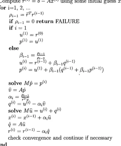
The original sequential algorithm is based on the Fast Multipole Method algo­ rithm adapted to the electromagnetic scattering problem. It uses an iterative scheme, the Conjugate Gradient Method (CGS) to solve the problem. In fact it concentrates on improving the matrix vector multiplication operation that is called twice in each loop in the iterative routine. Otherwise, for the part of preconditioning it uses the Sparse Library routines for factorization and trian­ gular solution of the sparse nearfield matrix. Moreover, it uses a template of a preconditioned CGS (Figure 4.1) from the LAPACK collection of templates]?].

Important to note in the algorithm of Figure 4.1 is that the matrix-vector multiplication and the preconditioning solve are both called twice in one itera­ tion. Since preconditioning was realized using a library function we will dwell

CHAPTER 4. TUB SEQUENTIAL IMPLEMENTATION OF THE SCATTERING SOLUTION 27

Compute = b — using some initial guess and choose f = fo r i = l , 2, ...

p ._ l

check convergence and continue if necessary en d

CHAPTER 4. THE SEQUENTIAL IMPLEMENTATION OF THE SCATTEB.ING SOLUTION 28

most in discussing the implementation of the matrix vector multiplication rou­ tine as actually this is where the Fast Multipole Method concept is utilized to speedup the operation.

4.4.1

Features of the Original Implementation

The following are highlights of the original solution

1. Factorization and the triangular solution for preconditioning the iterative routine to improve the iterative strategy convergence properties are real­ ized through the use of the Sparse library routines spFactor and spSolve respectively

2. Since the elements are indexed locally in the clusters, a global indexing scheme is used that gives a numbering to all elements using the element’s cluster number and its local, index in the cluster

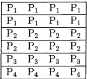
3. Zt^p is stored in a classical sparse matrix representation, that is, using three one dimensional arrays value^ row and column. Albeit transparent to the user, the library routine spFactor allocates memory space to store the factors of Z¡>4p that it uses in preconditioning.

4. Zpp is represented as a quadruplet of arrays that stand for the transfor­ mations required for the proceeding of the fast summation by the FMM. The basis and test functions are represented by two dimensional N x Np arrays Basis and Test. The upward and downward passes transforma­ tions are represented by a two dimensional N x Np array Prop. These two transformations require only one representation because they are conjugates of each other. The dimension Np represents the discretiza­ tion of the transformations for numerical computation. The translation of field eflFects between clusters is represented by a three dimensional M X M X Np array Trans. These bring up the amount of memory re­

quired to {32N+16M'^) X Np bytes where M is the number of the clusters

CHAPTER 4. THE SEQUENTIAL IMPLEMENTATION OF THE SCATTERING SOLUTION 29

5. The = Znf x x is made to progress the same order as the Z^f is

filled.

6. The spM X V hFF — Zff X performed according to the formulation of the FMM.

The original algorithm is given in Figure 4.2.

4.4.2

The Original Sequential Matrix Vector Multipli­

cation Algorithm

The objective of this algorithm is that given a matrix Z and vector I, determine the product v = Z -i, where Z is an x matrix and both v and i are size N vectors. Trivially, this involve 0{N^) operations and hence the FMM concept is used to reduce the complexity to 0(N^·^) as shown in Chapter 3.

The input to the program is data about a certain set of subscatters (or equivalently strips) which is arranged into clusters and the geometrical proper­ ties and relationships about the cluster data. Before calling the matrix-vector multiplication routine the data is converted into a matrix consisting of interac­ tions between the elements in the clusters. These interactions are classified into two forms depending on the amount of separation between them, the nearfield interaction and the far field interaction. The nearfield interaction is the one between elements in the same clusters and elements within clusters for which the separation is not enough to give the required accuracy if the FMM is used for their summation. The far field interaction is between elements in clusters that are separated enough for the FMM to be used to sum them up with the required accuracy.

In the matrix-vector multiplication the nearfield interaction is stored in a sparse matrix format and a direct sparse matrix - vector multiplication is performed between the near field matrix and the coefficient vector. Actually, the FMM algorithm is applied only to the far field interaction matrix.

CHAPTER 4. THE SEQUENTIAL IMPLEMENTATION OF THE SCATTERING SOLUTION ₃₀

for each cluster L do

for each discretization point ip do

initialize Q(ip, L) to zero

for each element 1 in cluster L do

get global index from array GI(L,1) let it be ig

for each discretization point ip do

Q(ip, L )=Q (ip, L)+Prop(ip,ig)*Basis(ip,ig)*x(ig) {Here is the end of the upward pass}

for each cluster K do

for each dicretization point ip do

initialize R(ip, K) to zero

for each cluster L do

if K and L are near clusters then for each discretization point ip do

R(ip, K )= R (ip , K)+Trans(ip, K, L) xQ( ip,L)

for each element k in cluster ,K do for each discretization point ip do

get global index from array GI(K, k) let it be ig initialize S(ip, ig) to zero

for each element k in cluster K do

get global index from array GI(K, k) let it be ig

for each discretization point ip do

S(ip, ig)=S(ip, ig) +conjg(Prop(ip, ig) )xR( ip,K)

for each element k in cluster K do

get global index from array GI(K, k) let it be ig initialize sum to zero

for each discretization point ip do

sum = sum + Test(ip,ig)xS(ip, ig)x weight (ip)

Figure 4.2: The Original Sequential Matrix Vector Multiplication {spMx V) Algorithm

CHAPTER 4. THE SEQUENTIAL IMPLEMENTATION OF THE SCATTERING SOLUTION 31

4.5

Modifications to the Original Sequential

Algorithm

Albeit the original purpose of our modifications to the sequential code was to have a much easily parallelizable algorithm, on examining the existing code carefully we realized several features of the existing implementation that could be improved for better performance in terms of time and space complexities of the algorithm. The main strategies that we used for improvement of the sequential code was to remove as much as possible floating point operations from the iteration loop body while utilizing the available cache in the best way possible. Theoretically, this would result into a constant change on the ultimate asymptotic complexity; practically, as exhibited from our experimental results, it gave rise to quite astonishing improvements in performance.

4.5.1

From Static to Dynamic Memory Management

An immediate limitation that we removed was lack of flexibility of space usage of the program. In the original version a large chunk was necessary to be allocated to the program before use, although only a small chunk of that space was actually used in the program. The main reason for this was absence of dynamic memory allocation in Fortran 77 standard. Initially when we were working on the Sun SparcStations we designed a C routine for this purpose and linked it with the other Fortran modules but later when we ported the implementation to the Parystec we converted the program into using the few Fortran 90 standard dynamic memory allocation routines that were available.

4.5.2

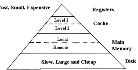
Cache Utilization

Cache utilization refers to reorganization of an algorithm so as to maximize running of the program at the top of the memory hierachy (Figure 6.3). This is realized by arranging the matrix data in form of interaction blocks. This was