2-D THRESHOLDING OF THE CONNECTIVITY MAP FOLLOWING THE
MULTIPLE SEQUENCE ALIGNMENTS OF DIVERSE DATASETS
Tunca Doğan1,3,*, Bilge Karaçalı2
1Biotechnology and Bioengineering Graduate Program, 2Electrical and Electronics Engineering Department, Izmir Institute of Technology and 3The Institute of Health Sciences, Dokuz Eylül University, Izmir, Turkey
*
[email protected], [email protected] ABSTRACT
Multiple sequence alignment (MSA) is a widely used method to uncover the relationships between the biomolecular sequences. One essential prerequisite to apply this procedure is to have a considerable amount of similarity between the test sequences. It’s usually not possible to obtain reliable results from the multiple alignments of large and diverse datasets. Here we propose a method to obtain sequence clusters of significant intragroup similarities and make sense out of the multiple alignments containing remote sequences. This is achieved by thresholding the pairwise connectivity map over 2 parameters. The first one is the inferred pairwise evolutionary distances and the second parameter is the number of gapless positions on the pairwise comparisons of the alignment. Threshold curves are generated regarding the statistical parameter values obtained from a shuffled dataset and probability distribution techniques are employed to select an optimum threshold curve that eliminate as much of the unreliable connectivities while keeping the reliable ones. We applied the method on a large and diverse dataset composed of nearly 18000 human proteins and measured the biological relevance of the recovered connectivities. Our precision measure (0.981) was nearly 20% higher than the one for the connectivities left after a classical thresholding procedure displaying a significant improvement. Finally we employed the method for the functional clustering of protein sequences in a gold standard dataset. We have also measured the performance, obtaining a higher F-measure (0.882) compared to a conventional clustering operation (0.827).
KEY WORDS
Biomedical Computing, Biostatistics, Sequence Analysis.
1. Introduction
Exploring evolutionary relationships between genes and proteins of biological organisms are crucial for discovering the physiological and molecular mechanisms govern their system. This is done by taking account of the molecular similarities and differences between these gene and protein sequences. In other words, the aim is to uncover the mutual history of these sequences by locating and exposing the molecular substitutions with respect to the most probable alignment between the nucleic acid or amino acid sequences.
The concept of sequence alignment was first applied to molecular biology decades ago to infer meaning from the complex sequential information. Alignment methods aim to uncover shared features between the tested sequences by identifying their molecular similarities. Needleman-Wunsch global alignment [1] and Smith–Waterman local alignment [2] algorithms are two basic tools used primarily in this manner. Nearly all current sophisticated tools are based upon these two pairwise alignment algorithms. Multiple Sequence Alignment (abbreviated and used as MSA from now on) algorithms are used for aligning more than two sequences. These tools came in the following years and still used widely. These methods are also based on the pairwise alignment procedure. A classical multiple sequence alignment operation basically consists of 2 steps. First one is the all-against-all pairwise alignment of input sequences. Second step is the progressive formation of the multiple alignment by introducing all sequences to the growing chain including the gaps inserted during the pairwise alignment step. Unlike pairwise local alignments, optimal solution is not guaranteed in the MSA procedure. Clustal family tools [3] (one of the most popular MSA methods) are for general use to align both nucleotide and amino acid sequences, and a typical example for the progressive alignment methods. ClustalW [3] is also used for phylogenetic tree construction. MUSCLE [4] incorporates iterations during which distance measures are refined, resulting in more accurate alignments. T-COFFEE [5] another common MSA method, uses the output from Clustal and local alignments to improve weighing factors. MAFFT [6] produces alignments in reduced computation times employing fast Fourier Transform [7]. A tremendous amount of progression was obtained in the field of sequence analysis for the past years thanks to these tools and they probably will serve the field for years to come.
One key prerequisite to acquire a meaningful output from the MSA procedure is to have a considerable amount of similarity between the input sequences. MSA algorithms shape the alignments around shared sequential features and when one or more of the input sequences lack this feature, these sequences cannot be aligned to the rest accurately in any way. The presence of non-homologous sequences sometimes misleads the propagation of the alignment and damage the output. This condition is especially reflected as errors on the phylogenetic trees drawn after the alignment. Remote sequences usually end up on irrelevant regions on the tree indicating false relations. Moreover, these sequences
may lead to inaccurate branch length predictions for the whole tree. As a result only the sequences that contain a specific feature -or features- are given to the procedure. This inhibits the analysis of large datasets composed of both similar and diverse biological sequences such as whole genomes or proteomes. An exhaustive preliminary study regarding the split of the dataset into highly similar sequence groups is usually necessary before the MSA process and this often is handled in a supervised manner using a BLAST like algorithm [8] and a vast database of confirmed known sequences. Even when there are no remote sequences in the dataset, the presence of fragments of homolog sequences (frequently encountered in online databases) usually leads to the same occasion due to the obscurity of the relations between the fragments.
Here we propose a method to make sense out of MSAs of datasets composed of sequences from different families (including the sequence fragments) using similarity thresholding with probability distribution techniques. At the end, the sequences are split into meaningful clusters in an unsupervised way using no information other than the sequences themselves. These sequence groups (consisting of homolog proteins) then can be subjected to the MSA process separately to obtain accurate alignments.
This is done by first, creating a new dataset by shuffling the elements of the original dataset and subjecting it to MSA procedure. Second, generating 2 D histograms consisting of pairwise evolutionary distances and the number of pairwise overlapped sites (number of positions without gaps) for the original and shuffled datasets separately. Third, drawing threshold curves on histograms using mean and standard deviation values of pairwise evolutionary distances. Fourth, calculating the probability distributions of discarding true and meaningless connections at each threshold; and decision making using a Receiver Operating Characteristics curve [9].
The method was applied on the MSA output of a large dataset consist of nearly 18000 human protein sequences. The dataset contained both similar and considerably distant -up to 100% sequence divergence- proteins. At the end of the procedure, the recovered connections were compared with the shared Gene Ontology associations [10] of these proteins to observe the biological relevance of the method. Finally, the method was employed to solve a common real world task: the functional clustering of protein sequences. A gold standard dataset [11] was analyzed by clustering the proteins sequences within, measuring the clustering performance and comparing it with a classical clustering operation.
The employed methods are expressed in detail in the next part of this article followed by the results and discussion part and a conclusion.
2. Methods
2.1 Shuffled Dataset Creation
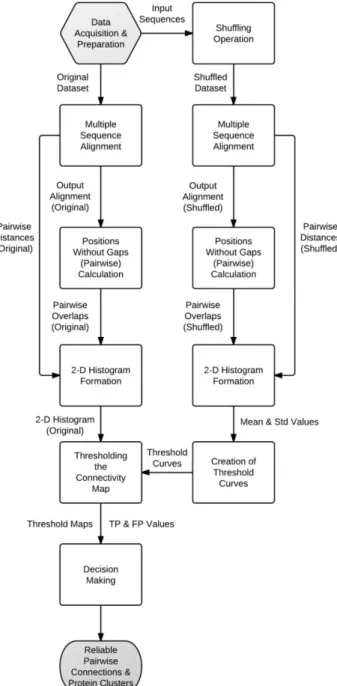
The flow chart of the proposed method is given in Figure 1.
Shuffled dataset was created by shuffling the elements of each amino acid sequence from the original dataset randomly. The shuffling operation was applied on the sequences separately so the length and amino acid composition of each sequence was preserved. The shuffled dataset contained the same number of sequences as the original dataset.
The shuffled dataset was used as a reference to represent unreliable connectivities that should be discarded. Since the elements of the sequences in this dataset were shuffled randomly, any inferred evolutionary relationships between these sequences were assumed to be emerged purely by chance.
2.2 Pairwise Evolutionary Distance Inference and the Calculation of Pairwise Alignment Overlaps
Right at the beginning of the procedure, we assumed that, there was a significant homology between all sequence pairs in the dataset. In other words, pairwise connectivity map was fully connected at the starting point. Most probably, some of the sequence pairs have no homology in-between, yet it was not known which ones at this point. What sought here was an indicator to measure the pairwise similarities to decide the existence or absence of significant homology. Pairwise evolutionary distance was a suitable measure to detect this similarity. Evolutionary distances close to zero, signal strong homology and as the distances increase, homology diminishes. Since it’s usually not possible to know the real evolutionary distances between biological sequences, they are inferred from the sequence distances using substitution models. In this analysis, evolutionary distances were inferred using Kimura amino acid substitution model [12] with the correction for multiple substitutions option.
In the multiple alignments of large datasets, the output alignment is usually quite lengthy. As a result, some of the sequences (especially short ones) may end up on different parts of the output alignment. It’s not possible to infer evolutionary distances of these proteins. In theory these sequences are diverged from a common ancestor so long before that the accumulated mutations makes it impossible to infer any similarity. At some other times, two distant sequences have matches (or mismatches) on a few positions (and there are gaps at the rest of the positions). After an inspection it was discovered that among all pairwise combinations in the output multiple alignments of test datasets, there were many occasions that only 1 or 2 sites were occupied by amino acid on both sequences -in other words gapless positions-. If this site gave a match, the evolutionary distance was inferred as zero between these 2 sequences since the remaining sites (including gaps) were not counted at all. However this information was not reliable as these sequences were not homologous. Figure 2 shows a sample case for this phenomenon. The rows represent 2 protein sequences taken out from a test Multiple Sequence Alignment output. The position shown in green color is the only site available for inferring the evolutionary distance. Since it’s a match, the distance was calculated as zero.
Figure 1. Flow diagram of the proposed method. Unreliable cases such as this one should be eliminated together with the connectivities with elevated pairwise distances. The proposed solution was eliminating the unreliable connections by thresholding the connectivity map over both pairwise evolutionary distances and the number of sites without gaps (pairwise overlaps). Similar to the pairwise evolutionary distances, the number of sites without gaps were calculated for each sequence pair in the original and the shuffled datasets.
Figure 2. A sample case that leads to an unreliable evolutionary distance inference in the MSA process.
2.3 2-D Histogram Formation
A 2-D histogram is a visual representation of the distribution of data just like a normal histogram. It differentiates from a normal histogram on the number of features the data is distributed upon. In a 2-D histogram, the distribution of the data is shown at the intersection of two feature intervals. In the plot, the discrete intervals of feature 1 are located on the horizontal axis and the ones for feature 2 are located on the vertical axis. One bin is formed for each feature 1 and feature 2 discrete interval combination and the number of points fall between the ranges of features for that bin appears inside. For the sake of visuality 2-D histograms are often created as intensity graphs instead of bars.
In this study, horizontal axis of the 2-D histogram represented the total number of gapless sites for each pairwise comparison -regarding the multiple alignment results-. Vertical axis represented the inferred pairwise distances. These axes were both divided into 100 discrete intervals making 10000 bins in total. In order to create the intensity contrast, grayscale colormap was chosen. More populated bins were represented by a darker color and sparsely populated bins by lighter colors.
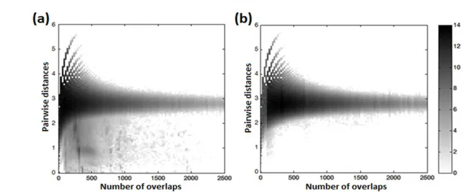
First, linearly scaled intervals were used for the colormap but resulted in visually poor plots. Later, a logarithmic scale was preferred for the coloring intervals producing satisfying visuality. Figure 3 shows 2-D histograms for the human protein dataset.
2.4 The Thresholding Operation
To create the threshold curves on the 2-D histograms, standard deviation and mean values of the distribution of ‘pairwise distances’ on each ‘number of sites without a gap’ interval was used. Equation 1 shows the formulation of the threshold curves.
(1)
Ti is the ith threshold curve, M is the mean pairwise distance –a constant value-, S is the standard deviation curve of the distribution of distances.
Standard deviation curve creation was carried out column-wise on 2-D histograms. For each discrete ‘number of sites without a gap’ interval, a standard deviation value was generated regarding the pairwise evolutionary distances. These successive values formed the standard deviation curve. In order to eliminate the noise on the curve, a normal (Gaussian) distribution model was fit on the curve [13]. The most suitable fit was found on the third order General Gaussian Model shown on Equation 2.
( ) [( )] [( )] [( )]
(2)
Coefficients were a1=0.34, b1=-37.29, c1=139.2, a2=0.2989, b2=-399.1, c2=589.9, a3=121.4, b3=-41610, c3=
16360 and for the goodness of the fit, R-square was found to be 0.9994.
Use of the standard deviation curves during the formation of the threshold curves allowed the capturing of the shape of the edge of the crowded portion in the 2-D histogram of the shuffled dataset. This was useful for separating the meaningless/unreliable connections from the reliable ones.
Using this method, 20 different threshold curves were created that scan the area below the mean distance curve. In addition to this set, 20 new curves were created to scan the area above the mean distance curve using the Equation 3 making 40 curves in total.
(3) To avoid confusion in curve names, all of these 40 curves were named as σ1,2,3,....,40. Figure 4 shows the
threshold curves on the 2-D histogram of the shuffled version of the human protein dataset.
2.5 Decision Making Step
A Receiver Operating Characteristic (ROC) curve [9] was employed in order to select the optimum threshold curve. Generally, a cut-off between the two classes (simply named as positives and negatives) with overlapping distributions is to be obtained using the ROC curve [9]. In our study, the positives group corresponded to the real connections from the original dataset whereas the negatives group corresponded to the random connections from the shuffled dataset. Motivation here is that, all connections coming from the shuffled dataset are assumed to be meaningless/unreliable; whereas, the ones from the original dataset contain both reliable and unreliable connections. To separate the reliable ones from the rest, a continuously increasing threshold was applied to the pairwise connections of both groups (using the previously generated curves) where the connections with the values exceeding this threshold were discarded. Presence of a pairwise connection indicates a significant homology between the sequence pair. When a connection is discarded, we assume that the corresponding sequences are non-homologs. At the optimum point, most of the connections from the shuffled dataset should be discarded and the ones left from the original set are accepted as the reliable connections.
To this end; true positives (TP), false positives (FP), true negatives (TN) and false negatives (FN) values were calculated from the number of real and random connections discarded and remained at each threshold together with the total number of real and random connections. The ROC curve was plotted using TP and FP rates. At this point, a cut-off should be decided regarding the slope of the ROC curve. For the automatic selection of the cut-off, the point where the slope equals to 105 or the point where all of the random connections were eliminated (whichever comes first) was chosen. Figure 5 shows the ROC curve for the human protein test dataset.
At this point, the connectivity map became disjointed due to the removal of inter-connections. This operation forms groups of homolog sequences.
2.5 Calculation of the Statistical Performance Measures Statistical measures were employed in order to evaluate the performance of the method on different tasks. These parameters consist of Recall, Precision and F-measure. Recall and Precision are composed of different combinations of TP, FP and FN values. F-measure incorporates both Recall and Precision to display the performance on a single parameter and frequently employed in clustering studies [14, 15, 16, 17]. The calculation of Recall (Sensitivity), Precision and F-measure are given in equations 4, 5 and 6 respectively.
( ) ( ) ( )
3. Results and Discussion
3.1 Analysis of the Large Human Protein Dataset Since the sequencing of human genome [18]; functions and interactions of genes and its products are being studied extensively throughout the world. This is a crucial subject and the key to develop novel medical solutions to prevalent diseases and other medical complications. Apart from expensive and laborious experimental studies, fundamentals of bioinformatics are applied to the case to infer answers. Statistical approaches are tried on these sequences to seek significant similarities between functionally known (experimentally proven) and unknown ones. In our study, we also prefer to apply our procedure on a large dataset composed of human protein sequences.
We decided to form our dataset regarding Gene Ontology (GO) associations [10]. Gene Ontology project aims the standard representation and documentation of genes and its products. The proteins annotated by GO have gone through a detailed inspection and examination process, as a result their functional associations are more reliable [10]. GO assign terms to these sequences on three main categories. Molecular function is the first one and represents the specific function of the sequence in the metabolism; biological process is the general operation during which this specific function is carried out; and cellular component is the location where this product functions. There is a hierarchical construction of these terms from broad to specific and a gene (or its product) is identified more clearly with growing number of associations. There is a clear indication of evolutionary and functional relatedness
(homology) between biological sequences with shared GO terms.
Up to date version of the accession numbers of Human proteins with GO associations were obtained from Gene Ontology project web site [10]. Protein sequences were downloaded from UniProt Database [19] via the accession numbers. Sequences with a length lower than 100 amino acids and higher than 10000 amino acids were assumed to be outliers and removed from the dataset. The final dataset consisted of nearly 18000 human protein sequences. This dataset was quite a hard case for any technique that relies on similarity measurements. Next, the shuffled dataset was created using randomly permuted elements of the amino acid sequences of the original dataset.
ClustalW2 v2.0.10 software package [3] was used for the global MSA procedure for the original and the shuffled datasets separately with the default options. Pairwise evolutionary distances were inferred using the built-in algorithm of ClustalW2 with Kimura amino acid substitution model [12] (with the correction for multiple substitutions option).
By comparison of the resulted alignments for the original and the shuffled datasets, it was observed that the length of the alignment was significantly shorter -in other words less gappy- for the shuffled dataset. This result was expected beforehand. Since no meaningful alignment can be obtained from the shuffled dataset any ways, MSA algorithm chose not to insert as many gaps as in the alignment of the original dataset in order to avoid gap costs. From the resulted alignments, 2-D histograms were created for the original and the shuffled datasets with the procedure described in the methods part.
The aim of thresholding the connectivity map was to eliminate the unreliable pairwise connections resulting from distant relationships or poor alignment. In a classical case with the MSA of a few closely related proteins, this procedure would be unnecessary since the probability of getting inaccurate pairwise alignments between closely related sequences are quite low. For this case, where there were nearly 18000 sequences that span nearly the entire
functional spectrum of the human proteins discovered so far, the resulted MSA was so long that especially some of the short sequences didn’t have any overlap on each other to calculate a pairwise distance. More misleading than that, some of these sequence pairs had an overlap on just 1 or 2 residues. If there was a match on that residue -since there were no other mismatches-, pairwise distance between these sequences ended up as zero, even though the rest of the sequences were quite diverged from each other. To solve this problem we introduce the thresholding of the connectivity map regarding 2 parameters (pairwise evolutionary distances and the total number of gapless sites on the pairwise comparison of the aligned sequences).
2-D histograms were created to this purpose for the shuffled and the original datasets. On these 2-D histograms, clumped regions were observed and the discrepancies between the histograms of the original and the shuffled datasets were tried to be extracted.
Figure 3 represents the 2-D histogram of the original dataset on the left (a) and shuffled dataset on the right (b) -both in log scale to increase visuality of the difference- where the horizontal axis represents the number of sites without gap intervals on pairwise comparisons and the vertical axis represents the pairwise evolutionary distance intervals. There was a visually distinct difference between the histograms around 0-2000 number of overlaps and 0-2 pairwise distances. This region on the original dataset histogram represents the reliable connections. However the region was not a clear cut as the shuffled datasets histogram also has representatives in the region. So this gray area should be handled with probability distribution techniques.
The threshold curves and the ROC curve were created following the procedures explained in the methods part. Figure 4 shows the threshold curves σ1,2,3,....,40 used for the
creation of the ROC curve, on the 2-D histogram of the shuffled dataset with the same horizontal and vertical axes.
The ROC curve (Figure 5) slope was selected to be 105 automatically for the cut-off. This point is shown with the black dot on the ROC curve (Figure 5). The threshold curve that yielded the selected cut-off was σ26. At this cut-off 270
meaningless (≈ 0% of the total) and 213000 real (0.14% of the total) connectivities were left on the connectivity map. At this point, it appeared like most of the connections from the original dataset were eliminated, however it’s crucial to mention that these were composed of false connections along with the true ones and our aim was to separate these two from each other.
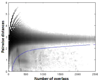
2-D histogram of the original dataset with the selected threshold curve plotted over (blue colored) is shown on Figure 6. All of the pairwise connectivities that had distance and overlap values above the curve were assumed to be unreliable and discarded.
Figure 4. Threshold curves σ1,2,3,....,40 on the 2-D histogram of
the shuffled version of human protein dataset. As expected, the threshold connectivity map became disjointed at this point and consisted of components with differing sizes. A component here is defined as a group of sequences that have either direct or indirect connections in-between. A manual examination over some sample components revealed that, each component was composed of similar proteins usually with significant homology.
Figure 5. The ROC curve for the thresholding operation of human protein dataset (black dot: selected threshold).
At this point in the study it was clear that, most of the inter-group distances were quite large, unreliable and
dumped during the thresholding operation. After the thresholding, 445 components were formed. The largest one contained 476 and the smallest ones contained 2 sequences.
In order to examine the biological relevance of our grouping, we tested our recovered true connections against the GO associations of the input sequences. We prepared the reference connection map by searching for the shared GO terms between sequences and assuming significant homology (existence of a connection) between these sequences. Any two sequences were assumed to be connected (related) when there was at least one shared GO term in-between. By this way, connections were formed between 37.9% of all possible sequence pairs. We measured performance by counting the true and false connections found in our analysis regarding the reference connections. When we got a connection that was also present in the reference map, we counted a true positive (TP). When we have a connection that didn’t appear in the reference, it was a false positive (FP). We calculated the precision measure (positive predictive value) as given in Equation 5. A precision value of 1 would mean all of the recovered connections were accurate. Our precision output was 0.981 whereas the same number of connections selected randomly resulted in 0.426 precision. Also to show how our method disposed meaningless connections, the same test was applied directly to the pairwise evolutionary distance (Kimura model) output of MSA procedure (a classical 1-D thresholding). The distance map was threshold with the disposal of the pairwise distances greater than 2. This was a reasonable value to assume homology and also the remaining number of connections in the map appeared to be nearly the same as our result providing the fair comparison of the performances. Precision for the classical thresholding over the pairwise distances was found as 0.799. The difference was nearly 20% in favor of our method which was a considerably significant improvement.
Figure 6. 2-D histogram of the original dataset with the selected threshold curve (σ26) plotted over.
The results supported our claim that thresholding the pairwise connectivity map over 2 dimensions (the number of positions without gaps in the pairwise comparisons of aligned sequences and inferred evolutionary distances) after
the MSA procedure assures the disposal of false homology detections and help make sense out of multiple alignments of large and mixed datasets. In addition, the detection of the potential MSA disrupters (distant sequences and homolog sequence fragments in the dataset) was provided by the proposed method.
3.2 Clustering of the Reference Dataset
Clustering of biomolecular sequences is an active area of research where the sequences are tried to be grouped under evolutionary and/or functional constraints in order to infer the history and functions of the unknown sequences (regarding the known ones). Over the last decade, many clustering algorithms were developed employing different statistical approaches. Some popular methods from the literature are TribeMCL [20], Spectral Clustering [14 & 15], FORCE [16] and TransClust [21].
At the final step of the study, members of a standard dataset composed of 866 manually curated enzymes (in 91 families) [11] were clustered and the accuracy of this application was measured (regarding the families that the sequences belong to) and compared with a classical thresholding operation incorporating only pairwise evolutionary distances. This conventional operation acting over 1 dimension takes part in most of the clustering methods (thresholding BLAST [8] e-values). This dataset is referred as a gold standard set in the literature and frequently employed in the testing of clustering algorithms [17, 21, 22]. By this way, the effectiveness of the proposed method in solving a real world task was displayed clearly.
First of all, the sequences were obtained via online material published by Brown et al. [11]. Next, the shuffled dataset was generated and both sets were subjected to MSA procedure using ClustalW2 v2.0.10 software package [3] with the default options. Then, the pairwise evolutionary distances were inferred using Kimura amino acid substitution model [12] (with the correction for multiple substitutions). After that, the numbers of overlapped positions on alignments were calculated, 2-D histograms were formed, and threshold and ROC curves were drawn as described in the Methods part. The cut-off was selected automatically at the point where no connections remained from the shuffled dataset. After the thresholding operation, sequences were clustered regarding the recovered pairwise connections. Since the presence of a connection between a sequence pair indicates a significant homology/similarity, these sequences appear in the same cluster. All sequences with a direct or an indirect connection in-between were grouped together. This approach was similar to the widely used graph theory method Connected Component Analysis [23] that was also employed in biomolecular sequence clustering methods frequently.
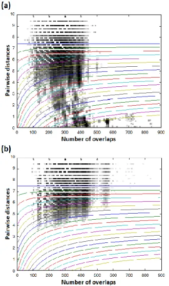
Figures 7 (a) and (b) show the 2-D histograms (with the threshold curves plotted over) of the original reference dataset and its shuffled version respectively (in log scale). The true/reliable connections are visible on Figure 7 with dark color just over the baseline of the x-axis. Figure 8 shows the curves for the classical 1-D thresholding
operation on the 2-D histogram of the original reference dataset. Notice the curves here are linear and parallel to x-axis since this operation did not incorporate number of overlapped positions.
Figure 7. 2-D threshold curves on the 2-D histograms of (a) the original and (b) the shuffled standard dataset
Figure 8. 1-D threshold curves on the 2-D histogram of the original standard dataset
Table 1 shows the Precision, Recall and F-measure values for the clustering performance of the conventional 1-D thresholding operation (first column) and the proposed method (second column) using the threshold curve selected automatically. For a fair comparison between the proposed method and the conventional thresholding operation, the average clustering performances regarding all threshold curves are given in the third and fourth columns. Best F-measures are given in bold. As seen from Table 1, the clustering performance was increased nearly 6.5% (F-measure: 0.827 to 0.882) when the proposed method was employed instead of the conventional thresholding with the automatically selected threshold curve. On the other hand, the average clustering performance was increased around 7.9% (F-measure: 0.712 to 0.768) with our method. These results indicate the effectiveness of the proposed approach in the functional clustering of amino acid sequences.
Table 1. Clustering performance measures for the standard dataset after the conventional (1-D) and 2-D thresholding
operations.
At the selected curve Average of all curves
1-D Thres. 2-D Thres. 1-D Thres. 2-D Thres.
Precision 0.711 0.794 0.700 0.723
Recall 0.990 0.991 0.892 0.935
F-measure 0.827 0.882 0.712 0.768
4. Conclusion
In this study we proposed a procedure to infer meaningful pairwise homology relationships and to obtain clusters of homolog sequences from MSAs (including the alignments of large datasets composed of diverged sequences). The pairwise connectivity map was threshold over 2 dimensions (inferred evolutionary distances and the number of gapless positions on pairwise comparisons of the aligned sequences) with curves considering the mean and standard deviation values of the random dataset. This random dataset was composed of the shuffled elements of the sequences of the original set. The method was applied on a large dataset composed of nearly 18000 human protein sequences. A precision value of 0.981 was measured for the biological relevance of the recovered pairwise connections. This value was nearly 20% higher than the precision measured right after the MSA. Finally, protein sequences in a gold standard dataset were clustered using the proposed method along with the measurement of the clustering performance. The results displayed improvement in clustering accuracy (F-measure: 0.8819 with the automatic threshold selection) compared to the classical thresholding over inferred evolutionary distances (F-measure: 0.8274). These results indicate the potential of the proposed method both in recovering true pairwise similarity relationships after MSAs and the functional clustering of biomolecular sequences. In the time ahead, we plan to implement this thresholding procedure in a comprehensive method for the functional clustering of the sequences with the identification of the domain regions within.
References
[1] S.B. Needleman, & C.D. Wunsch, A general method applicable to the search for similarities in the amino acid sequence of two proteins, Journal of Molecular Biology 48(3), 1970, 443– 53.
[2] T.F. Smith, & M.S. Waterman, Identification of Common Molecular Subsequences, Journal of Molecular Biology 147, 1981, 195–197.
[3] M.A. Larkin, G. Blackshields, N.P. Brown, R. Chenna, P.A. McGettigan, H. McWilliam, F. Valentin, I.M. Wallace, A. Wilm, R. Lopez., J.D. Thompson, T.J. Gibson, & D.G. Higgins, ClustalW and ClustalX version 2, Bioinformatics 23(21), 2007, 2947-2948. [4] R.C. Edgar, MUSCLE: multiple sequence alignment with high accuracy and high throughput, Nucleic Acids Research 32(5), 2004, 1792–97.
[5] C. Notredame, D.G. Higgins, J. Heringa, T-Coffee: A novel method for fast and accurate multiple sequence alignment, Journal
of Molecular Biology 302(1), 2000, 205–217.
[6] K. Katoh, & H. Toh, Recent developments in the MAFFT multiple sequence alignment program, Briefings in Bioinformatics
9(4), 2008, 286-298.
[7] E.O. Brigham, The Fast Fourier Transform (New York: Prentice-Hall, 2002)
[8] S.F. Altschul, et al., Gapped BLAST and PSI-BLAST: a new generation of protein database search programs, Nucleic Acids
Research 25, 1997, 3389-3402.
[9] T.A. Lasko, J.G. Bhagwat, K.H. Zou, & L. Ohno-Machado, The use of receiver operating characteristic curves in biomedical informatics, Journal of Biomedical Informatics 38(5), 2005, 404– 415.
[10] The Gene Ontology Consortium, Gene ontology: tool for the unification of biology, Nat. Genet., 25(1), 2000, 25-9.
[11] S.D. Brown, et al., A gold standard set of mechanistically diverse enzyme superfamilies. Genome Biology 7, 2006, R8. [12] M. Kimura, The neutral theory of molecular evolution (Cambridge, UK: Cambridge University Press, 1983).
[13] W. Bryc, The normal distribution: characterizations with
applications (Heidelberg, Germany: Springer-Verlag, 1995).
[14] A. Paccanaro, et al., Spectral clustering of protein sequences,
Nucleic Acids Research 34, 2006, 1571-1580.
[15] T. Nepusz, et al., SCPS: a fast implementation of a spectral method for detecting protein families on a genome-wide scale,
BMC Bioinformatics 11, 2010, 120.
[16] T. Wittkop, et al., Large scale clustering of protein sequences with FORCE -A layout based heuristic for weighted cluster editing,
BMC Bioinformatics 8, 2007, 396.
[17] L. Apeltsin, et al., Improving the quality of protein similarity network clustering algorithms using the network edge weight distribution, Bioinformatics 27, 2011, 326-33.
[18] J.C. Venter, et al., The sequence of the human genome,
Science 291, 2001, 1304-1351.
[19] The UniProt Consortium, Reorganizing the protein space at the Universal Protein Resource (UniProt), Nucleic Acids Research
40, 2012, 71-75.
[20] A.J. Enright, et al., An efficient algorithm for large-scale detection of protein families, Nucleic Acids Research 30, 2002, 1575–1584.
[21] T. Wittkop, et al., Partitioning biological data with transitivity clustering, Nature Methods 7, 2010, 419-20.
[22] V. Miele, et al., High-quality sequence clustering guided by network topology and multiple alignment likelihood,
Bioinformatics 28, 2012, 1078-85.
[23] R. Diestel, Graph Theory (Heidelberg, Germany: Springer-Verlag, 2010).
View publication stats View publication stats